Graviton production in non-inflationary cosmology

Abstract

We discuss the creation of massless particles in a Universe, which transits from a radiation-dominated era to any other expansion law. We calculate in detail the generation of gravitons during the transition to a matter-dominated era. We show that the resulting gravitons generated in the standard radiation/matter transition are negligible. We use our result to constrain one or more previous matter-dominated era, or any other expansion law, which may have taken place in the early Universe. We also derive a general formula for the modification of a generic initial graviton spectrum by an early matter dominated era.

I Introduction

One of the most interesting aspect of inflation is that it leads to the generation of a scale-invariant spectrum of scalar perturbations slava and of gravitational waves staro (see also slavaBook ; myBook ). The origin of these perturbations is the quantum generation of field correlations in a time-dependent background (scalar field modes for the scalar perturbations and gravitons for the tensor perturbations). Since this generation takes place mainly on super-horizon scales, it is not correct to talk of ’particles’. However, long after inflation, when the perturbations re-enter the horizon, the particle concept, e.g. for gravitons becomes meaningful and we can calculate, e.g. the energy density of the gravitons which have been generated during inflation.

It is natural to ask whether particle production takes place also in an ordinary expanding but non-inflationary Friedmann Universe. The answer is that particle production (or more generically the quantum generation of field correlations) can indeed take place after inflation, but if there is no inflationary phase to start with, the initial vacuum state is in general not known, and the production rate cannot be computed. Examples where particle creation taking place after inflation (or after pre-big bang) modifies the final spectrum are given in Refs. pbb1 ; pbb2 ; VS2 ; VS3 . Especially in Ref. VS2 it has been studied how inflationary perturbations are modified if the subsequent expansion is not standard radiation but some other expansion law.

In general, the vacuum state, and hence the particle concept, is well defined only if the spacetime is static or very slowly varying BirDav . Let us consider a mode of fixed (comoving) frequency $k$ in a Friedmann universe. The above condition then corresponds to $k/\mathcal{H}\gg 1$, where $\mathcal{H}=aH$ is the comoving Hubble scale. In this sense, the scale (wavelength) under consideration must be “inside the horizon”. However, the production of a particle with a given energy $k$ can only take place if the energy scale of expansion is larger or of the order of the energy of the associated mode, i.e. $k\,\raisebox{-2.58334pt}{$\buildrel<\over{\sim}$}\,\mathcal{H}$. Therefore, having a well defined initial vacuum state, and subsequent particle creation, usually requires a decreasing comoving Hubble rate. This is verified only during inflation or during a collapsing Friedmann Universe, like in the pre-big bang or in bouncing models.

However, one important exception to this general rule exists, and it is the subject of the present paper: in a radiation-dominated Friedmann background, massless perturbations do not couple to the expansion of the Universe, and evolve like in ordinary Minkowski space. This has already been realized and studied to some extent in Ref. grish . In a radiation-dominated Universe we therefore can provide vacuum initial conditions for all modes of a massless field, including super-horizon modes. Thus, when the expansion law changes, e.g. from radiation- to matter-dominated, the massless modes couple to the expansion of the Universe, and those with $k/\mathcal{H}<1$ are amplified.

In this paper we study this phenomenon in two situations of interest. In the first, we investigate graviton production during the ordinary radiation/matter transition at redshift $z_{\mathrm{eq}}\simeq 3500$. We determine the amplitude and the spectrum of the generated gravity wave background, and we show that the spectrum is flat and the amplitude is negligibly small. In the second case, we investigate the production of gravitons during an arbitrary matter-dominated phase, which could take place in the early Universe, e.g., if a (very weakly interacting) particle becomes massive, and succeeds to dominate the Universe for a period of time before it decays into radiation. We derive a general formula for the gravity wave spectrum generated by any number of such intermediate periods of matter domination. We also determine the gravity waves produced by a transition into an arbitrary other expansion law. Finally, we discuss the modifications of our results which occur when the initial state is not the vacuum but some arbitrary state which may already contain particles. In this work we concentrate on graviton production, but all our results are equally applicable to other massless particles.

The reminder of this paper is organized as follows. In the next section we present the setup and the basic formulae used in our work. In Section III, we calculate the gravitational wave production during the standard radiation/matter transition. We also give the results for the transition from radiation to some generic expansion law. In Section IV we consider the effect of one or several additional transitions in the early Universe and we derive results for general non-vacuum initial conditions. In Section V we derive the consequences of our results and we draw some conclusions.

Notation: We work in a spatially flat Friedmann Universe, and we denote conformal time by $t$, so that

$$ds^{2}=a^{2}(t)\left(-dt^{2}+\delta_{ij}dx^{i}dx^{j}\right)~{}.$$

An over-dot denotes the derivative with respect to the conformal time. We use natural units $c=\hbar=1$, except for Newton’s constant $G$, which is related to the reduced Planck mass by $8\pi G=m_{p}^{-2}$. We normalize the scale factor, so that $a_{0}=a(t_{0})=1$ at the present time.

II Graviton creation in cosmology

We now consider tensor perturbations of the Friedmann metric, namely

$$ds^{2}=a^{2}(t)\left[-dt^{2}+(\delta_{ij}+2h_{ij})dx^{i}dx^{j}\right]~{},$$

where $h_{ij}$ is a transverse and traceless tensor. In Fourier space we have

$$h_{ij}(\mathbf{k},t)=h_{+}(k,t)e^{(+)}_{ij}(\hat{\mathbf{k}})+h_{-}(k,t)e^{(-)}_{ij}(\hat{\mathbf{k}})\ ,$$ (1)

where $e^{(\pm)}_{ij}(\hat{\mathbf{k}})$ denote the positive and negative helicity polarization tensors, and $k^{i}e^{(\pm)}_{ij}=0$. In a perfect fluid background, i.e. if there are no anisotropic stresses, both amplitudes satisfy the same wave equation,

$$\Box h=\ddot{h}+2\frac{\dot{a}}{a}\dot{h}+k^{2}h=0\ ,$$ (2)

where $h\equiv h_{\pm}$. This equation of motion is obtained when expanding the gravitational action in a Friedman universe to second order in $h$,

$$S+\delta S=-\frac{m_{p}^{2}}{2}\int d^{4}x\sqrt{-(g+\delta g)}(R+\delta R)~{}.$$ (3)

A brief calculation shows that the lowest (second order) contribution to $\delta S$ can be written in Minkowski-space canonical form,

$$\delta S^{(2)}=-\frac{1}{2}\int d^{4}x\left(\partial_{\mu}\phi\partial^{\mu}\phi-\frac{\ddot{a}}{a}\phi^{2}\right)=\int d^{4}x{\cal L}\,,$$ (4)

if we rescale $h$ as

$$h(\mathbf{x},t)={1\over\sqrt{2}\,m_{p}a(t)}\phi(\mathbf{x},t)\ .$$ (5)

Eq. (4) is the action of a canonical scalar field with time-dependent effective squared mass $m^{2}(t)=-\ddot{a}/a$. If the expansion of the Universe is slow enough (compared to the frequency of the mode under consideration), then the effective mass is negligible, and the theory describes a massless scalar field in Minkowski space, which can be quantized according to the usual procedure: we first promote the field to an operator

$$\hat{\phi}(\mathbf{x},t)=\int\frac{d^{3}k}{(2\pi)^{3}}\left[e^{i\mathbf{k}\cdot\mathbf{x}}\chi_{\mathbf{k}}(t)\hat{b}_{\mathbf{k}}+e^{-i\mathbf{k}\cdot\bf{x}}\chi_{\mathbf{k}}^{*}(t)\hat{b}_{\mathbf{k}}^{\dagger}\right]\ ,$$ (6)

then we impose the commutation rules

$$[b_{\mathbf{k}},b^{\dagger}_{\mathbf{k}^{\prime}}]=(2\pi)^{3}\delta^{3}(\mathbf{k}-\mathbf{k}^{\prime})\ ,\quad[b_{\mathbf{k}},b_{\mathbf{k}^{\prime}}]=[b^{\dagger}_{\mathbf{k}},b^{\dagger}_{\mathbf{k}^{\prime}}]=0\,.$$

The field equations derived from the action (4) lead to the mode equation

$$\ddot{\chi}_{\mathbf{k}}+\left[k^{2}-\frac{\ddot{a}}{a}\right]\chi_{\mathbf{k}}=0\,.$$ (7)

Within linearized gravity we can therefore quantize the metric fluctuations, provided the Universe expands adiabatically, by making use of the above rescaling of the amplitude $h$.

In particular, we now assume that the Universe is initially radiation-dominated, so that $a(t)=t$, and $\ddot{a}/a=0$, and $\phi$ represents exactly a massless scalar field in Minkowski space. We consider the vacuum initial conditions for the modes $\chi_{\mathbf{k}}(t)$ as given by

$$\chi_{\mathbf{k}}(t)=\frac{1}{\sqrt{2k}}e^{-ikt}\ .$$ (8)

More general initial conditions will be considered at the end of Sec. IV. The field normalization is determined by the Klein-Gordon norm

$$i\chi^{*}\stackrel{{\scriptstyle\leftrightarrow}}{{\partial_{0}}}\chi\equiv i(\chi^{*}\partial_{0}\chi-\chi\partial_{0}\chi^{*})=1~{}.$$ (9)

Then, the field operator $\hat{\phi}$ and its canonically conjugate momentum, $\hat{\Pi}=\partial{\cal L}/\partial{(\partial_{0}\hat{\phi})}$ satisfy the canonical commutation relations. The operators $\hat{b}_{\mathbf{k}}$ define the $in$ vacuum by $\hat{b}_{\mathbf{k}}|0_{\rm in}\rangle=0~{}\forall\mathbf{k}$. In the following, this is the initial vacuum, void of particles by construction.

Suppose now that at a time $t=t_{1}$, the Universe changes abruptly from radiation-dominated to another expansion law. Then, the effective squared mass no longer vanishes, and the initial modes, with $kt_{1}<1$ are amplified. Continuity requires that $\chi$ and $\dot{\chi}$ match at $t=t_{1}$, and these conditions determine the Bogoliubov coefficients, which relate the new modes $\chi_{\rm out}$ and operators $\hat{b}_{\mathbf{k}\rm,out}$ to the old ones, $\chi_{\rm in}$ and $\hat{b}_{\mathbf{k}\rm,in}$ by BirDav

$$\chi_{\rm out}(t) = \alpha\chi_{\rm in}(t)+\beta\chi^{*}_{\rm in}(t)\ ,$$ (10)

$$\hat{b}_{\rm out} = \alpha^{*}\hat{b}_{\rm in}-\beta^{*}\hat{b}^{\dagger}_{\rm in}\ .$$ (11)

With these relations, we can compute the number density of the particles created at the transition BirDav

$$N(k,t_{1})=\langle 0_{\rm in}|\hat{b}^{\dagger}_{\mathbf{k},\,\rm out}\hat{b}_{\mathbf{k},\,\rm out}|0_{\rm in}\rangle=|\beta|^{2}\ .$$ (12)

Thus, the energy density $\rho\equiv\langle T^{0}{}_{0}\rangle$ can be written as

$$\rho_{h}={1\over a^{4}}\int{d^{3}k\over(2\pi)^{3}}kN(k,t_{1})={1\over 2\pi^{2}a^{4}}\int dkk^{3}|\beta|^{2}\ ,$$ (13)

which implies the usual formula

$${d\rho_{h}\over d\log k}\Big{|}_{\rm tot}={k^{4}|\beta|^{2}\over\pi^{2}a^{4}}\ ,$$ (14)

where we have multiplied Eq. (13) by a factor 2 to take into account both polarizations. Note also that $k$ denotes comoving momenta/energy so that we had to divide by $a^{4}$ to arrive at the physical energy density. The second quantity of interest is the power spectrum $P_{h}(k,t)$, defined by

$$4\pi\int{dk\over k}P_{h}(k,t)=\langle 0_{\rm in}|h(t,\mathbf{x})^{2}|0_{\rm in}\rangle\ .$$ (15)

Using Eqs. (5) and (6), we obtain

$$P_{h}(k,t)={k^{2}|\beta|^{2}\over(2\pi)^{3}m_{p}^{2}a^{2}}\ ,$$ (16)

where, again, we have multiplied by 2 to account for both polarizations.

Note that for all this it is not important that we consider a spin 2 graviton. The exactly same mode equation is obtained for a scalar field and also for a fermion field. In the latter case, the commutation relations have to be replaced by the corresponding anti-commutation relations.

III From radiation to matter era

Before discussing a transition from the radiation-dominated era to the matter era, let us consider the transition from radiation to some generic power law expansion phase, $a\propto t^{q}$ with $q\neq 1$ at some time $t_{1}$. In the new era $\ddot{a}/a=q(q-1)/t^{2}\neq 0$. Note that only if $q>1$ (or if $q<0$ which corresponds to inflation or contraction), so that $m^{2}(t)=-q(q-1)/t^{2}$ is negative, we will have significant particle production. Since the expansion law is related to the equation of state parameter $w=P/\rho$ via myBook

$$q=\frac{2}{1+3w}\,,$$ (17)

this requires $w<1/3$.

Let us start in the vacuum during the radiation era, then $\chi$ is given entirely by the negative frequency modes, Eq. (8). This means that we consider the situation where there are no significant gravity waves present from an earlier inflationary epoch. Here, we really want to study the production due solely to the radiation/matter transition. The general solution of the mode equation (7) in the new era are the spherical Hankel functions AS of order $q-1$,

$$\chi_{\mathbf{k}}(t) = \frac{\alpha_{1}}{\sqrt{2k}}zh_{q-1}^{(2)}(z)+\frac{\beta_{1}}{\sqrt{2k}}zh_{q-1}^{(1)}(z)$$ (18)

where $z=kt$. Note that inside the horizon, i.e. for $z\gg 1$, $zh^{(2)}_{q-1}(z)\propto\exp(-iz)$ corresponds to the negative frequency modes while $zh^{(1)}_{q-1}(z)\propto\exp(iz)$ corresponds to positive frequency modes. We match $\chi$ and $\dot{\chi}$ at $t=t_{1}$ to the radiation-dominated vacuum solution (8). A brief calculation yields the coefficients ($z_{1}\equiv kt_{1}$)

$$\alpha_{1} = -\frac{i}{2}e^{-iz_{1}}\left[(iz_{1}+q)h^{(1)}_{q-1}(z_{1})-z_{1}h_{q}^{(1)}(z_{1})\right]\,,$$ (19)

$$\beta_{1} = -\frac{i}{2}e^{-iz_{1}}\left[(iz_{1}+q)h^{(2)}_{q-1}(z_{1})-z_{1}h_{q}^{(2)}(z_{1})\right]\,.$$ (20)

This instantaneous matching condition is good enough for frequencies for which the transition is rapid, i.e. $z_{1}\ll 1$. In fact, for frequencies with $z_{1}>1$, the transition is adiabatic and no particle creation will take place. This can also been seen when considering the limits of the above result for large $z_{1}$. Then $\alpha_{1}\rightarrow 1$ and $\beta_{1}\rightarrow 0$, but strictly speaking the above approximations are not valid in this regime where no particle creation takes place. We therefore concentrate on $z_{1}\ll 1$.

Let us now study the specific case of the radiation–matter transition, i.e. $q=2$. Then we have to consider spherical Hankel functions of order 1 and the solution is given by

$$\chi_{\mathbf{k}}(t)=\frac{\alpha_{1}}{\sqrt{2k}}\frac{z-i}{z}e^{-iz}+\frac{\beta_{1}}{\sqrt{2k}}\frac{z+i}{z}e^{iz}\,.$$ (21)

The matching at $t_{1}$ now yields

$$\alpha_{1}=1+\frac{i}{z_{1}}-\frac{1}{2z_{1}^{2}}\,,\qquad\beta_{1}=-\frac{1}{2z_{1}^{2}}\,e^{-2iz_{1}}~{}.$$ (22)

We want to evaluate the quantum field $\hat{\phi}$ at late time, when $z\gg 1$ and the mode $k$ under consideration is sub-horizon. Then, the solution (21) is again the Minkowski solution,

$$\chi_{\mathbf{k}}(t)\simeq\frac{\alpha_{1}}{\sqrt{2k}}e^{-iz}+\frac{\beta_{1}}{\sqrt{2k}}e^{iz}~{}.$$ (23)

The number of gravitons generated during the matter era (before $z\gg 1$) is, see Eq. (12)

$$N(k,t) = |\beta_{1}|^{2}\,.$$ (24)

The graviton power spectrum is given by Eq. (16), and the energy density by Eq. (13).

Using that $\rho_{\mathrm{rad}}a^{4}\equiv\rho_{\mathrm{rad}}(t_{1})a_{1}^{4}=\frac{3}{2}m_{p}^{2}\mathcal{H}_{1}^{2}a_{1}^{2}$ and $|\beta_{1}|^{2}=z_{1}^{-4}/4$, we obtain

$$\frac{d\Omega_{h}(k)}{d\log k} = \frac{2\Omega_{\mathrm{rad}}}{3\pi^{2}}\frac{k^{4}}{m_{p}^{2}\mathcal{H}_{1}^{2}a_{1}^{2}}|\beta_{1}|^{2}=\frac{\Omega_{\mathrm{rad}}}{6\pi^{2}}\left(\frac{H_{1}}{m_{p}}\right)^{2}$$ (25)

$$= \Omega_{\mathrm{rad}}\frac{g_{\mathrm{eff}}}{36\times 30}\left(\frac{T_{1}}{m_{p}}\right)^{4}~{}.$$

For the second equal sign we have used that $\mathcal{H}_{1}=1/t_{1}=a_{1}H_{1}$, which is strictly true only in the radiation era, in the matter era we have $\mathcal{H}=2/t$ and at the transition a value between $1$ and $2$ would probably be more accurate. But within our approximation of an instant transition, we do not bother about such factors. For the last equal sign we used $H_{1}^{2}=\rho_{\mathrm{rad}}/(6m_{p}^{2})$ with $\rho_{\mathrm{rad}}=g_{\mathrm{eff}}\frac{\pi^{2}}{30}T^{4}$ where $g_{\mathrm{eff}}=N_{B}+\frac{7}{8}N_{F}$ is the effective number of degrees of freedom.

For a generic transition we obtain $|\beta_{1}|^{2}=z_{1}^{-2q}/4$ so that

$$\frac{d\Omega_{h}(k)}{d\log k}\simeq\Omega_{\mathrm{rad}}\left(\frac{T_{1}}{m_{p}}\right)^{4}z_{1}^{4-2q}~{}.$$ (26)

This spectrum is blue (i.e. growing with $k$) if $q<2$ and red otherwise.

As $z_{1}<1$ in the regime of validity of our formula, we need a red spectrum i.e. $q>2$ to enhance the gravitational wave energy density with respect to the result from the radiation $\rightarrow$ matter transition. According to Eq. (17), this requires $-1/3<w<0$, a slightly negative pressure, but still non-inflationary expansion.

In the standard radiation to matter transition when three species of left handed neutrinos and the photon are the only relativistic degrees of freedom, we have $g_{\mathrm{eff}}=29/4$. For this transition

$$T_{1}=T_{\mathrm{eq}}\simeq 0.85\mathrm{eV}\simeq 0.35\times 10^{-27}m_{p}\,,$$

hence the result (25) is completely negligible.

IV More than one radiation-matter transition

We now consider an early matter dominated era. At some high temperature $T_{1}\gg T_{\mathrm{eq}}$, corresponding to a comoving time $t_{1}$, a massive particle may start to dominate the Universe and render it matter-dominated. At some later time $t_{2}$, corresponding to temperature $T_{2}$, this massive particle decays and the Universe becomes radiation-dominated again, until the usual radiation–matter transition, which takes place at $T_{\mathrm{eq}}\equiv T_{3}$. We want to determine the gravitational wave spectrum and the spectral density parameter $d\Omega_{h}/d\log(k)$ as functions of $T_{1}$ and $T_{2}$.

Let us first again start with the vacuum state in the radiation eta before $t_{1}$. When, we just obtain the results (22) for the Bogoliubov coefficients $\alpha_{1}$ and $\beta_{1}$ after the first transition. To evaluate the matching conditions at the second transition, matter to radiation, we set

$$\chi=\frac{\alpha_{2}}{\sqrt{2k}}e^{-ikt}+\frac{\beta_{2}}{\sqrt{2k}}e^{ikt}\,,\quad t\geq t_{2}\,.$$

Matching $\chi$ and $\dot{\chi}$ at $t_{2}$ we can relate the new coefficients $\alpha_{2}$ and $\beta_{2}$ to $\alpha_{1}$ and $\beta_{1}$. A brief calculation gives

$$\alpha_{2} = \alpha_{1}\left(1-\frac{i}{z_{2}}-\frac{1}{2z_{2}^{2}}\right)+\frac{\beta_{1}}{2z_{2}^{2}}e^{2iz_{2}}$$ (27)

$$= \alpha_{1}f(z_{2})+\beta_{1}g(z_{2})\,,$$

$$\beta_{2} = \beta_{1}\left(1+\frac{i}{z_{2}}-\frac{1}{2z_{2}^{2}}\right)+\frac{\alpha_{1}}{2z_{2}^{2}}e^{-2iz_{2}}$$ (28)

$$= \beta_{1}\bar{f}(z_{2})+\alpha_{1}\bar{g}(z_{2})~{},$$ (29)

or in matrix notation

$$\left(\begin{array}[]{c}\alpha_{2}\\ \beta_{2}\end{array}\right) = {M}(z_{2})\left(\begin{array}[]{c}\alpha_{1}\\ \beta_{1}\end{array}\right)\,,\qquad\mbox{with}$$ (34)

$${M}(z) = \left(\begin{array}[]{cc}f(z)&g(z)\\ \bar{g}(z)&\bar{f}(z)\end{array}\right)$$ (37)

$${M}^{-1}(z) = \left(\begin{array}[]{cc}\bar{f}(z)&-g(z)\\ -\bar{g}(z)&f(z)\end{array}\right)\ .$$ (40)

The fact that $M\in Sl(2,\mathbb{C})$, i.e., $|f(z)|^{2}-|g(z)|^{2}=1$ ensures that the normalization condition (9) which translates to the condition $|\alpha|^{2}-|\beta|^{2}=1$ for the Bogolioubov coefficients of a free field, is maintained at the transition. Finally, the matching at the usual radiation–matter transition yields

$$\alpha_{3} = \alpha_{2}\left(1+\frac{i}{z_{3}}-\frac{1}{2z_{3}^{2}}\right)-\frac{\beta_{2}}{2z_{3}^{2}}\,e^{2iz_{3}}~{},$$

$$\beta_{3} = \beta_{2}\left(1-\frac{i}{z_{3}}-\frac{1}{2z_{3}^{2}}\right)-\frac{\alpha_{2}}{2z_{3}^{2}}\,e^{-2iz_{3}}~{},$$ (41)

$$\left(\begin{array}[]{c}\alpha_{3}\\ \beta_{3}\end{array}\right) = M^{-1}(z_{3})\left(\begin{array}[]{c}\alpha_{2}\\ \beta_{2}\end{array}\right)$$ (46)

$$\left(\begin{array}[]{c}\alpha_{3}\\ \beta_{3}\end{array}\right) = M^{-1}(z_{3})M(z_{2})M^{-1}(z_{1})\left(\begin{array}[]{c}1\\ 0\end{array}\right)\,.$$ (51)

To obtain the power spectrum and energy density in this case, we simply have to replace $|\beta|^{2}$ in Eqs. (16) and (14) by $|\beta_{3}|^{2}$. In Fig. 1 we plot $|\beta_{3}|^{2}$ as a function of $z_{3}$ for different choices of $t_{2}$. The instantaneous transition approximation breaks down for $z_{3}>1$, hence only the left side of the vertical line is physical. For the right side one would have to solve the mode equation numerically, but since we know that particle production is suppressed for these frequencies, we do not consider them. We concentrate on $z_{3}\leq 1$. For these wave numbers, also $z_{1}<z_{2}<z_{3}<1$.

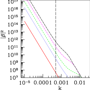
Figure 1: The Bogoliubov coefficient $|\beta_{3}(k)|^{2}$ for $t_{1}=1$, and $t_{3}=2000$, with various values of $t_{2}$. Only the k-values left of the vertical dashed line satisfy $kt_{3}<1$. They show clearly a $k^{-4}$ slope and the amplitude is well approximated by (54).

This allows the following approximations,

$$\alpha_{1}\simeq\beta_{1}\simeq-\frac{1}{2z_{1}^{2}}\,,\quad z_{1}\ll 1$$ (52)

$$\alpha_{2}\simeq-\beta_{2}\simeq\frac{iz_{2}}{3z_{1}^{2}}\,,\quad z_{2}\ll 1$$ (53)

$$\alpha_{3}\simeq\beta_{3}\simeq-\frac{2z_{2}}{3z_{1}^{2}z_{3}}\,,\quad z_{3}\ll 1\,.$$ (54)

To obtain the results (53) and (54) we have to expand the exact expression (27) to fourth order and (41) to second order, but we consider only the largest term in the result given above, using also $z_{1}<z_{2}<z_{3}$. Therefore, in the approximate expression (53), where we have neglected a term proportional to $z_{1}/z_{2}^{2}$, one no longer sees that $\alpha_{2}\rightarrow 1$ and $\beta_{2}\rightarrow 0$ when $t_{2}\rightarrow t_{1}$ and hence $z_{2}\rightarrow z_{1}$. In this case there is no intermediate matter-dominated era and therefore no particle creation, hence $\beta_{2}=0$. This can be seen from the exact expression given in Eq. (27).

Within these approximations, Eqs. (16) and (14) lead to

$$P_{h}(k) = \frac{1}{(2\pi)^{3}}\left(\frac{t_{2}}{m_{p}at_{1}^{2}t_{3}k}\right)^{2}\,,\quad kt_{3}<1$$ (55)

$$\frac{d\Omega_{h}}{d\log k} = \frac{\Omega_{\mathrm{rad}}}{\pi^{2}}\frac{k^{4}|\beta_{3}|^{2}}{a_{1}^{4}\rho_{\mathrm{rad}}(t_{1})}$$

$$= \Omega_{\mathrm{rad}}\frac{g_{\mathrm{eff}}(T_{1})}{18\times 45}\left(\frac{T_{1}}{m_{p}}\right)^{4}\left(\frac{T_{\mathrm{eq}}}{T_{2}}\right)^{2}\,,~{}kt_{\mathrm{eq}}<1\,.$$

This result can be generalized to several, say $N$, intermediate radiation $\rightarrow$ matter transitions at times $t_{2n-1}$ and back to radiation at time $t_{2n}$, $1\leq n\leq N$, with the result

$$|\beta_{2N+1}|^{2}\simeq\frac{1}{(kt_{1})^{4}}\left(\frac{T_{3}\cdots T_{2N-1}T_{\mathrm{eq}}}{T_{2}\cdots T_{2N}}\right)^{2}\,.$$ (57)

Hence, each return to the radiation-dominated era at some intermediate temperature $T_{2n}$ leads to a suppression factor $(T_{2n+1}/T_{2n})^{2}$, where $T_{2n+1}$ denotes the temperature at the start of the next matter era.

On large scales, $kt_{\mathrm{eq}}<1$, the energy density spectrum is flat. The best constraints on an intermediate radiation-dominated era therefore come from the largest scales, i.e. from observations of the cosmic microwave background (CMB) as we shall discuss in the next section.

We now briefly consider the case when the initial conditions differ from the vacuum case, Eq. (8). We assume an arbitrary initial state of the field given by

$$\chi_{\mathbf{k}}(t)=\frac{\alpha_{0}}{\sqrt{2k}}e^{-ikt}+\frac{\beta_{0}}{\sqrt{2k}}e^{ikt}\ ,$$ (58)

together with the normalization condition which ensures that the field is canonically normalized, $|\alpha_{0}|^{2}-|\beta_{0}|^{2}=1$. The same calculations as above now yield

$$\left(\begin{array}[]{c}\alpha_{3}\\ \beta_{3}\end{array}\right) = M^{-1}(z_{3}){M}(z_{2})M^{-1}(z_{1})\left(\begin{array}[]{c}\alpha_{0}\\ \beta_{0}\end{array}\right)\,,$$ (63)

where $M(z)$ is the matrix giving the transition from matter to radiation defined in Eq. (37).

Expanding this in $z_{1}$, $z_{2}$ and $z_{3}$, using $z_{1}<z_{2}<z_{3}<1$ one finds that to lowest non-vanishing order, the final result for $\beta_{3}$ depends only $|\alpha_{0}+\beta_{0}|$. However, if the phase of $\alpha_{0}$ and $\beta_{0}$ are nearly opposite, i.e., $\alpha_{0}\simeq-\beta_{0}$ , and if $|\alpha_{0}|$ and therefore also $|\beta_{0}|$ are much larger than $1$, a correction proportional to $|\alpha_{0}-\beta_{0}|$ becomes important. More precisely, the last of Eqs. (52) now is replaced by

$$\beta_{3}\simeq{2z_{2}\over 3z_{1}z_{3}}\left[-\frac{1}{z_{1}}(\alpha_{0}+\beta_{0})+2i(\alpha_{0}-\beta_{0})\right]\ .$$ (64)

If $\alpha_{0}=1$ and $\beta_{0}=0$, the second term can be neglected with respect to the first one and we reproduce the previous result (54). As we see from this equation, a large phase difference between $\alpha_{0}$ and $\beta_{0}$ changes not only the amplitude but also the slope of the spectrum. Of course in concrete examples, like for a previous inflationary period, see Ref. VS2 , the coefficients $\alpha_{0}$ and $\beta_{0}$ also depend on the wavenumber.

In Fig. 2 we show the dependence of $|\beta_{3}|^{2}$ on $|\alpha_{0}|$ for different values of the relative phase between $\alpha_{0}$ and $\beta_{0}$ (top panel) and as a function of the relative phase for different values of $|\alpha_{0}|$. The difference of $|\beta_{3}|^{2}$ between the case where $\alpha_{0}$ and $\beta_{0}$ are perfectly in phase and of opposite phase is of the order of $1/z_{1}$, if $|a_{0}|$ is significantly larger than $1$. This is already evident from Eq. (64). In the Fig. 2 we have chosen $z_{1}=0.1$, a unrealistically high value, in order to have a better visibility of the phase dependence which then changes $|\beta_{3}|^{2}$ only by one order of magnitude.

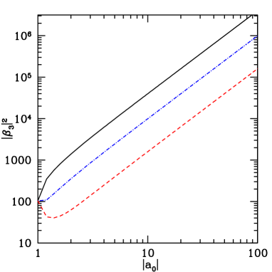
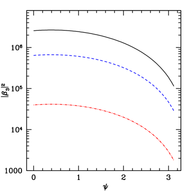
Figure 2: In the top panel we show $|\beta_{3}|^{2}$ as a function of $\alpha_{0}$ for $\alpha_{0}$ and $\beta_{0}$ in phase (top, solid, black line), of opposite phase (lowest, dashed, red line) and with a phase difference of $0.8\pi$ (middle, dot-dashed, blue line).
In the bottom panel we show $|\beta_{3}|^{2}$ as a function of the phase difference $\psi$ for $|\alpha_{0}|=80$ (top line) $|\alpha_{0}|=40$ (middle line) and $|\alpha_{0}|=10$ (lowest line). We have chosen $z_{1}=0.1$ in this plot and the overall vertical normalization is in units of $\left(2z_{2}/(z_{1}z_{3})\right)^{2}$.

In conclusion, in the case of a non-vacuum initial state, $|\alpha_{0}|$ significantly larger than $1$, graviton production is enhanced typically by a factor of order $|\alpha_{0}|^{2}\sim|\beta_{0}|^{2}$ which is the number of initial particles. Hence in addition to the spontaneous creation we now also have induced particle creation which is proportional to the initial particle number and much larger than the spontaneous creation if the particle number is large. An interesting point is that the phase shift between $\alpha_{0}$ and $\beta_{0}$ can significantly affect the final spectrum.

V Discussion and Conclusions

The fact that the observed CMB anisotropies are of the order of $10^{-5}$ yields a strong limit on gravitational waves with wave numbers of the order of the present Hubble scale, see e.g. bb .

$$\left.\frac{d\Omega_{h}}{d\log k}\right|_{k=H_{0}}<10^{-15}\,.$$ (65)

With $\Omega_{\mathrm{rad}}\simeq 10^{-5}$, and Eq. (LABEL:e:res2), this implies the limit

$$\left(\frac{T_{1}}{m_{p}}\right)^{2}\frac{T_{\mathrm{eq}}}{T_{2}}<10^{-5}\,.$$ (66)

We know that during nucleosynthesis the Universe was radiation-dominated, hence $T_{2}\geq 0.1$MeV. With $T_{\mathrm{eq}}\sim 1$eV, the above inequality reduces to $T_{1}<m_{p}$ for the value $T_{2}\simeq 0.1$MeV, and it is even less stringent for higher values of $T_{2}$. Hence even though the production of gravitons during an intermediate matter era is of principal interest, we cannot derive stringent limits on $T_{1}$ and $T_{2}$. On the other hand, for values of $T_{1}$ and $T_{2}$ close to the maximal respectively minimal value, $T_{1}\sim m_{p}$ and $T_{2}\sim 0.1$MeV, these gravitons would leave a detectable signature in the cosmic microwave background.

We can, however, use this effect to limit any intermediate era with $q>2$, i.e. $-1/3<w=P/\rho<0$. According to Eq. (26), in the general case, the particle number is of the order of $|\beta_{1}|^{2}\simeq z_{1}^{-2q}$, so that

$$\frac{d\Omega_{h}}{d\log k}\simeq\Omega_{\mathrm{rad}}(kt_{1})^{4-2q}\left(\frac{T_{1}}{m_{p}}\right)^{4}\left(\frac{T_{\mathrm{eq}}}{T_{2}}\right)^{2}\ ,\quad z_{1}\ll 1\,.$$ (67)

As above, $T_{2}$ denotes the temperature at which the Universe returns to the radiation-dominated state, hence nucleosynthesis requires $T_{2}>0.1$MeV. In this case, if $q>2$, the spectrum becomes red and, at $k\sim H_{0}$, the limit can become quite interesting. Hence, graviton production can significantly limit a (non-inflationary) phase with negative pressure in the early universe. For $k=H_{0}$, using $t_{1}=\mathcal{H}_{1}^{-1}=1/(a_{1}H_{1})$, we obtain

$$(H_{0}t_{1})^{-1}\simeq\left(\frac{g_{\mathrm{eff}}(T_{1})}{10^{5}}\right)^{1/2}\left(\frac{T_{1}}{T_{0}}\right)^{3}\,,$$

where $T_{0}\simeq 0.2\times 10^{-4}$eV is the present temperature of the Universe. This can be a significant factor for large values of $T_{1}$. Inserting this expression in Eq. (67), the limit (65) yields

$$\left(\frac{g_{\mathrm{eff}}(T_{1})}{10^{5}}\right)^{q-2}\left(\frac{T_{1}}{T_{0}}\right)^{6(q-2)}\left(\frac{T_{1}}{m_{p}}\right)^{4}\left(\frac{T_{\mathrm{eq}}}{T_{2}}\right)^{2}\,\raisebox{-2.58334pt}{$\buildrel<\over{\sim}$}\,10^{-10}~{}.$$ (68)

For example, for $w=-1/21$, ($q=7/3$), we already obtain

$$\frac{T_{1}}{T_{2}}\left(\frac{T_{1}}{m_{p}}\right)^{2}\,\raisebox{-2.58334pt}{$\buildrel<\over{\sim}$}\,10^{-9}\,.$$ (69)

E.g. for $T_{2}=1$MeV this implies $T_{1}<10^{8}$GeV. For smaller values of $w$ the limit becomes more stringent.

In this paper we have shown that there is cosmological particle production of massless modes whenever the expansion law is not radiation-dominated so that $\ddot{a}/a\neq 0$. This term acts like a time-dependent mass and leads to the production of modes with comoving energy $k^{2}<|\ddot{a}/a|\simeq\mathcal{H}^{2}$, hence with physical energy $\omega=k/a\,\raisebox{-2.58334pt}{$\buildrel<\over{\sim}$}\,H$. One readily sees that particle production is significant only if $q<1$, i.e. the squared mass $-\ddot{a}/a<0$. When starting from a radiation-dominated Universe, we do have a well defined initial vacuum state also for the super-horizon modes which can be amplified by a transition to another expansion law. We have also given the expressions for the produced particle number in the case of a generic, non-vacuum initial state, Eq. (64). This can be applied to an arbitrary inflationary, pre-big bang or bouncing model, which may already contain gravitons before the first radiation era.

We have explicitly calculated the production of gravitons for a vacuum initial state and have arrived at the following main conclusions:

• The gravitons produced after the standard radiation–matter transition are completely negligible.

• If we introduce a matter-dominated era in the early universe, this leads to a flat energy spectrum of gravity waves which, in the most optimistic case, can be sufficient to contribute to the CMB tensor anisotropies in an observable way.

• A phase of expansion with $-1/3<w<0$ leads to a red spectrum of gravitons. Such a phase in the early universe is severely constrained mainly by the amplitude of CMB anisotropies.

• A graviton spectrum present at the beginning of the radiation era can become significantly amplified and modified by intermediate not-standard evolution of the universe.

Acknowledgment: We thank John Barrow for valuable comments. This work is supported by the Swiss National Science Foundation.

References

- (1) V. F. Mukhanov and G. V. Chibisov, Sov. Phys. JETP 56 (1982) 258 [Zh. Eksp. Teor. Fiz. 83 (1982) 475].
- (2) A. A. Starobinsky, JETP Lett. 30 (1979) 682 [Pisma Zh. Eksp. Teor. Fiz. 30 (1979) 719].
- (3) V. Mukhannov, Physical Foundations of Cosmology, Cambridge University Press (2005).
- (4) R. Durrer, The Cosmic Microwave Background, Cambridge University Press (2008).
- (5) R. Durrer, M. Gasperini, M. Sakellariadou and G. Veneziano, Phys. Lett. B 436 (1998) 66 [arXiv:astro-ph/9806015].
- (6) R. Durrer, M. Gasperini, M. Sakellariadou and G. Veneziano, Phys. Rev. D 59 (1999) 043511 [arXiv:gr-qc/9804076].
- (7) V. Sahni, Phys. Rev. D 42 (1990) 453.
- (8) V. Sahni, M. Sami and T. Souradeep, Phys. Rev. D 65 (2002) 023518 [arXiv:gr-qc/0105121].
- (9) N. D. Birrell and P. C. W. Davies, Quantum Fields In Curved Space, Cambridge University Press (1982).
- (10) L. P. Grishchuk, Sov. Phys. JETP 40 (1975) 409 [Zh. Eksp. Teor. Fiz. 67 (1974) 825].
- (11) M. Abramowitz and I. Stegun, Handbook of Mathematical Functions, Dover Publications (New York, 1972, ninth Ed.).
- (12) L. A. Boyle and A. Buonanno, Phys. Rev. D 78, 043531 (2008) [arXiv:0708.2279 [astro-ph]].