Optimal control as a graphical model inference problem

Abstract

We reformulate a class of non-linear stochastic optimal control problems introduced by Todorov, (2007) as a Kullback-Leibler (KL) minimization problem. As a result, the optimal control computation reduces to an inference computation and approximate inference methods can be applied to efficiently compute approximate optimal controls. We show how this KL control theory contains the path integral control method as a special case. We provide an example of a block stacking task and a multi-agent cooperative game where we demonstrate how approximate inference can be successfully applied to instances that are too complex for exact computation. We discuss the relation of the KL control approach to other inference approaches to control.

1 Introduction

Stochastic optimal control theory deals with the problem to compute an optimal set of actions to attain some future goal. With each action and each state a cost is associated and the aim is to minimize the total future cost. Examples are found in many contexts such as motor control tasks for robotics, planning and scheduling tasks or managing a financial portfolio. The computation of the optimal control is typically very difficult due to the size of the state space and the stochastic nature of the problem.

The most common approach to compute the optimal control is through the Bellman equation. For the finite horizon discrete time case, this equation results from a dynamic programming argument that expresses the optimal cost-to-go (or value function) at time $t$ in terms of the optimal cost-to-go at time $t+1$. For the infinite horizon case, the value function is independent of time and the Bellman equation becomes a recursive equation. In continuous time, the Bellman equation becomes a partial differential equation.

For high dimensional systems or for continuous systems the state space is huge and the above procedure cannot be directly applied. A common approach to make the computation tractable is a function approximation approach where the value function is parameterized in terms of a number of parameters (Bertsekas and Tsitsiklis,, 1996). Another promising approach is to exploit graphical structure that is present in the problem to make the computation more efficient (Boutilier et al.,, 1995; Koller and Parr,, 1999). However, this graphical structure is in general not inherited by the value function, and thus the graphical representation of the value function may not be appropriate.

In this paper, we introduce a class of stochastic optimal control problems where the control is expressed as a probability distribution $p$ over future trajectories given the current state and where the control cost can be written as a Kullback-Leibler (KL) divergence between $p$ and some interaction terms. The optimal control is given by minimizing the KL divergence, which is equivalent to solving a probabilistic inference problem in a dynamic Bayesian network. The optimal control is given in terms of (marginals of) a probability distribution over future trajectories. The formulation of the control problem as an inference problem directly suggests exact inference methods such as the Junction Tree method (JT) (Lauritzen and Spiegelhalter,, 1988) or a number of well-known approximation methods, such as the variational method (Jordan,, 1999), belief propagation (BP) (Murphy et al.,, 1999), the cluster variation method (CVM) or generalized belief propagation (GBP) (Yedidia et al.,, 2001) or Markov Chain Monte Carlo (MCMC) sampling methods. We refer to this class of problems as KL control problems.

The class of control problems considered in this paper is identical as in Todorov, (2008, 2007, 2009), who shows that the Bellman equation can be written as a KL divergence of probability distributions between two adjacent time slices and that the Bellman equation computes backward messages in a chain as if it were an inference problem. The novel contribution of the present paper is to identify the control cost with a KL divergence instead of making this identification in the Bellman equation. The immediate consequence is that the optimal control problem is identical to a graphical model inference problem that can be approximated using standard methods.

We also show how KL control reduces to the previously proposed path integral control problem (Kappen,, 2005) when noise is Gaussian in the limit of continuous space and time. This class of control problem has been applied to multi-agent problems using a graphical model formulation and junction tree inference in Wiegerinck et al., (2006, 2007) and approximate inference in van den Broek et al., 2008b ; van den Broek et al., 2008a . In robotics, Theodorou et al., (2009); Theodorou et al., 2010a ; Theodorou et al., 2010b has shown the the path integral method has great potential for application. They have compared the path integral method with some state-of-the-art reinforcement learning methods, showing very significant improvements. In addition, they have successful implemented the path integral control method to a walking robot dog. The path integral approach has recently been applied to the control of character animation (da Silva et al.,, 2009).

2 Control as KL minimization

Let $x=1,\ldots,N$ be a finite set of states, $x^{t}$ denotes the state at time $t$. Denote by $p^{t}(x^{t+1}|x^{t},u^{t})$ the Markov transition probability at time $t$ under control $u^{t}$ from state $x^{t}$ to state $x^{t+1}$. Let $p(x^{1:T}|x^{0},u^{0:T-1})$ denote the probability to observe the trajectory $x^{1:T}$ given initial state $x^{0}$ and control trajectory $u^{0:T-1}$.

If the system at time $t$ is in state $x$ and takes action $u$ to state $x^{\prime}$, there is an associated cost $\hat{R}(x,u,x^{\prime},t)$. The control problem is to find the sequence $u^{0:T-1}$ that minimizes the expected future cost

$$C(x^{0},u^{0:T-1}) =\sum_{x^{1:T}}p(x^{1:T}|x^{0},u^{0:T-1})\sum_{t=0}^{T}\hat{R}(x^{t},u^{t},x^{t+1},t)$$

$$=\left\langle\sum_{t=0}^{T}\hat{R}(x^{t},u^{t},x^{t+1},t)\right\rangle$$ (1)

with the convention that $\hat{R}(x^{T},u^{T},x^{T+1},T)=R(x^{T},T)$ is the cost of the final state and $\langle\rangle$ denotes expectation with respect to $p$. Note, that $C$ depends on $u$ in two ways: through $\hat{R}$ and through the probability distribution of the controlled trajectories $p(x^{1:T}|x^{0},u^{0:T-1})$.

The optimal control is normally computed using the Bellman equation, which results from a dynamic programming argument (Bertsekas and Tsitsiklis,, 1996). Instead, we will consider the restricted class of control problems for which $C$ in Equation (1) can be written as a KL divergence. As a particular case, we consider that $\hat{R}$ is the sum of a control dependent term and a state dependent term. We further assume the existence of a ’free’ (uncontrolled) dynamics $q^{t}(x^{t+1}|x^{t})$, which can be any first order Markov process that assigns zero probability to physically impossible state transitions.

We quantify the control cost as the amount of deviation between $p^{t}(x^{t+1}|x^{t},u^{t})$ and $q^{t}(x^{t+1}|x^{t})$ in KL sense. Thus,

$$\hat{R}(x^{t},u^{t},x^{t+1},t)=\log\frac{p^{t}(x^{t+1}|x^{t},u^{t})}{q^{t}(x^{t+1}|x^{t})}+R(x^{t},t)\qquad t=0,\ldots,T-1$$ (2)

with $R(x,t)$ an arbitrary state dependent control cost. Equation (1) becomes

$$C(x^{0},p) =KL(p||\psi)$$

$$=\sum_{x^{1:T}}p(x^{1:T}|x^{0})\log\frac{p(x^{1:T}|x^{0})}{\psi(x^{1:T}|x^{0})}$$

$$=KL(p||q)+\langle{R}\rangle$$ (3)

$$\psi(x^{1:T}|x^{0}) =q(x^{1:T}|x^{0})\exp\left(-\sum_{t=0}^{T}R(x^{t},t)\right)$$ (4)

Note, that $C$ depends on the control $u$ only through $p$. Thus, minimizing $C$ with respect to $u$ yields: $0=\frac{dC}{du}=\frac{dC}{dp}\frac{dp}{du}$, where the minimization with respect to $p$ is subject to the normalization constraint $\sum_{x^{1:T}}p(x^{1:T}|x^{0})=1$. Therefore, a sufficient condition for the optimal control is to set $\frac{dC}{dp}=0$. The result of this KL minimization is well known and yields the “Boltzmann distribution”

$$p(x^{1:T}|x^{0}) =\frac{1}{Z(x_{0})}\psi(x^{1:T}|x^{0})$$ (5)

and the optimal cost

$$C(x^{0},p) =-\log Z(x^{0})=-\log\sum_{x^{1:T}}q(x^{1:T}|x^{0})\exp\left(-\sum_{t=0}^{T}R(x^{t},t)\right)$$ (6)

where $Z(x^{0})$ is a normalization constant (see Appendix A). In other words, the optimal control solution is the (normalized) product of the free dynamics and the exponentiated costs. It is a distribution that avoids states of high $R$, at the same time deviating from $q$ as little as possible. Note that since $q$ is a first order Markov process, $p$ in Equation (5) is a first order Markov process as well.

The optimal control in the current state $x^{0}$ at the current time $t=0$ is given by the marginal probability

$$p(x^{1}|x^{0}) =\sum_{x^{2:T}}p(x^{1:T}|x^{0})$$ (7)

This is a standard graphical model inference problem, with $p$ given by Equation (5). Since $\psi$ is a chain, we can compute $p(x^{1}|x^{0})$ by backward message passing:

$$\beta^{T}(x^{T}) =1$$

$$\beta^{t}(x^{t}) =\sum_{x^{t+1}}\psi_{t}(x^{t},x^{t+1})\beta^{t+1}(x^{t+1})$$

$$p(x^{t+1}|x^{t}) \propto\psi^{t}(x^{t},x^{t+1})\beta^{t+1}(x^{t+1}).$$

The interpretation of the Bellman equation as message passing for the KL control problems was first established in Todorov, (2008). The difference between the KL control computation and the standard computation using the Bellman equation is schematically illustrated in Figure 1.

Dynamics: $p^{t}(x^{t}|x^{t-1},u^{t-1})$	$\rightarrow$ dynamic programming $\rightarrow$	Bellman Equation
Cost: $C(x^{0},u)=\left\langle\hat{R}\right\rangle$		Cost-to-go: $J(x^{0})$
$\downarrow$		$\downarrow$
restricted class of problems		approximate $J$
$\downarrow$		$\downarrow$
Dynamics: $p^{t}(x^{t}|x^{t-1})$	$\rightarrow$ approximate inference $\rightarrow$	approximation
$C(x^{0},p)=KL(p||\psi)$		of optimal $u$

Figure 1: Overview of the approaches to computing the optimal control. Top left) The general optimal control problem is formulated as a state transition model $p$ that depends on the control (or policy) $u$ and a cost $C(u)$ that is the expected $\hat{R}$ with respect to the controlled dynamics $p$. The optimal control is given by the $u$ that minimizes a cost $C(u)$. Top right) The traditional approach is to introduce the notion of cost-to-go or value function $J$, which satisfies the Bellman equation. The Bellman equation is derived using a dynamic programming argument. Bottom right) For large problems, an approximate representation of $J$ is used to solve the Bellman equation which yields the optimal control. Bottom left) The approach in this paper is to consider a class of control problems for which $C$ is written as a KL divergence. The computation of the optimal control (optimal $p$) becomes a statistical inference problem, that can be approximated using standard approximate inference methods.

The optimal cost, Equation (6), is minus the log partition sum and is the expectation value of the exponentiated state costs $\sum_{t=0}^{T}R(x^{t},t)$ under the uncontrolled dynamics $q$. This is a surprising result, because it means that we have a closed form solution for the optimal cost-to-go $C(x^{0},p)$ in terms of the known quantities $q$ and $R$.

A result of this type was previously obtained in Kappen, (2005) for a class of continuous non-linear stochastic control problems. Here, we show that a slight generalization of this problem ($g_{ai}(x,t)=1$ in Kappen, (2005)) is obtained as a special case of the present KL control formulation. Let $x$ denote an $n$-dimensional real vector with components $x_{i}$. We define the stochastic dynamics

$$dx_{i} =f_{i}(x,t)dt+\sum_{a}g_{ia}(x,t)(u_{a}dt+d\xi_{a})$$ (8)

with $f_{i}$ an arbitrary function, $d\xi_{a}$ an $m$-dimensional Gaussian process with covariance matrix $\left\langle d\xi_{a}d\xi_{b}\right\rangle=\nu_{ab}dt$ and $u_{a}$ an $m$-dimensional control vector. The distribution over trajectories is given by

$$p(x^{dt:T}|x^{0},u^{0:T-dt}) =\prod_{s=0}^{T-dt}\mathcal{N}(x^{s+dt}|x^{s}+(f^{s}+g^{s}u^{s})dt,g^{s}\nu(g^{s})^{T}dt)$$ (9)

with $f^{t}=f(x^{t},t)$ and the distribution over trajectories under the uncontrolled dynamics is defined as $q(x^{dt:T}|x^{0})=p(x^{dt:T}|x^{0},u^{0:T-dt}=0)$.

For this particular choice of $p$ and $q$, the control cost in Equation (3) becomes (see Appendix B for a derivation)

$$C(x,u(t\rightarrow T)) =\left\langle\phi(x(T))+\int_{t}^{T}ds\frac{1}{2}u(x(s),s)^{T}\nu^{-1}u(x(s),s)+R(x(s),s)\right\rangle$$ (10)

where $\langle\rangle$ denotes expectation with respect to the controlled dynamics $p$, where the sums become integrals and where we have defined $\phi(x)=R(x,T)$.

Equations (8) and (10) define a stochastic optimal control problem. The solution for the optimal cost-to-go for this class of control problems can be shown to be given as a so-called path integral, an integral over trajectories, which is the continuous time equivalent of the sum over trajectories in Equation (6). Note, that the cost of control is quadratic in $u$, but of a particular form with the matrix $\nu^{-1}$ in agreement with Kappen, (2005). Thus, the KL control theory contains the path integral control method as a particular limit. As is shown in Kappen, (2005), this class of problems admits a solution of the optimal cost-to-go as an integral over paths, which is similar to Equation (6).

2.1 Graphical model inference

In typical control problems, $x$ has a modular structure with components $x=x_{1},\ldots,x_{n}$. For instance, for a multi-joint arm, $x_{i}$ may denote the state of each joint. For a multi-agent system, $x_{i}$ may denote the state of each agent. In all such examples, $x_{i}$ itself may be a multi-dimensional state vector. In such cases, the optimal control computation, Equation (7), is intractable. However, the following assumptions are likely to be true:

• The uncontrolled dynamics factorizes over components

  $$q^{t}(x^{t+1}|x^{t})=\prod_{i=1}^{n}q_{i}^{t}(x^{t+1}_{i}|x^{t}_{i})$$

• The interaction between components has a (sparse) graphical structure $R(x,t)=\sum_{\alpha}R_{\alpha}(x_{\alpha},t)$ with $\alpha$ a subset of the indices $1,\ldots,n$ and $x_{\alpha}$ the corresponding variables.

Typical examples are multi-agent systems and robot arms. In both cases the dynamics of the individual components (the individual agents and the different joints, respectively) are independent a priori. It is only through the execution of the task that the dynamics become coupled.

Thus, $\psi$ in Equation (4) has a graphical structure that we can exploit when computing the marginals in Equation (7). For instance, one may use the junction tree (JT) method, which can be more efficient than simply using the backward messages. Alternatively, we can use any of a large number of approximate graphical model inference methods to compute the optimal control. In the following sections, we will illustrate this idea by applying several approximate inference algorithms in two different tasks.

3 Stacking blocks (KL-blocks-world)

Consider the example of piling blocks into a tower. This is a classic AI planning task (Russell et al.,, 1996). It will be instructive to see how a variant of this problem is solved as a stochastic control problem, As we will see, the optimal control solution will in general be a mixture over several actions. We define the KL-blocks-world problem in the following way: let there be $n$ possible block locations on the one dimensional ring (line with periodic boundaries) as in Figure 2,

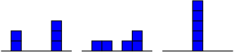
Figure 2: Block stacking problem: the objective can be (but is not restricted to) to stack the initial block configuration (left) into a single stack (right) through a sequence of single block moves to adjacent positions (middle).

and let $x^{t}_{i}\geq 0,i=1,\ldots,n,t=0,\ldots,T$ denote the height of stack $i$ at time $t$. Let $m$ be the total number of blocks.

At iteration $t$, we allow to move one block from location $k^{t}$ and move it to a neighboring location $k^{t}+l^{t}$ with $l^{t}=-1,0,1$ (periodic boundary conditions). Given $k^{t},l^{t}$ and the old state $x^{t-1}$, the new state is given as

$$x^{t}_{k^{t}} =x^{t-1}_{k^{t}}-1$$ (11)

$$x^{t}_{k^{t}+l^{t}} =x^{t-1}_{k^{t}+l^{t}}+1$$ (12)

and all other stacks unaltered. We use the uncontrolled distribution $q$ to implement these allowed moves. For the purpose of memory efficiency, we introduce auxiliary variables $s^{t}_{i}=-1,0,1$ that indicate whether the stack height $x_{i}$ is decremented, unchanged or incremented, respectively. The uncontrolled dynamics $q$ becomes $q(k^{t})={\cal U}(1,\ldots,n)$, $q(l^{t})={\cal U}(-1,0,+1)$,

$$q(s^{t}|k^{t},l^{t}) =\prod_{i=1}^{n}q(s^{t}_{i}|k^{t},l^{t})$$

$$q(s^{t}_{i}|k^{t},l^{t}) =\begin{cases}\delta_{s^{t}_{i},-1}&\text{for $k^{t}=i,l^{t}=\pm 1$}\\ \delta_{s^{t}_{i},+1}&\text{for $k^{t}+l^{t}=i,l^{t}=\pm 1$}\\ \delta_{s^{t}_{i},0}&\text{otherwise}\end{cases},$$

where $\cal U(\cdot)$ denotes the uniform distribution. The transition from $x^{t-1}$ to $x^{t}$ is a mixture over the values of $k^{t},l^{t}$:

$$q(x^{t}|x^{t-1}) =\sum_{k^{t},l^{t}}\prod_{i=1}^{n}q(x^{t}_{i}|x^{t-1}_{i},k^{t},l^{t})q(k^{t})q(l^{t})$$ (13)

$$q(x^{t}_{i}|x^{t-1}_{i},k^{t},l^{t}) =\sum_{s_{i}^{t}}q(x^{t}_{i}|x^{t-1}_{i},s^{t}_{i})q(s^{t}_{i}|k^{t},l^{t})$$ (14)

$$q(x^{t}_{i}|x^{t-1}_{i},s^{t}_{i}) =\delta_{x_{i}^{t},x_{i}^{t-1}+s^{t}_{i}}$$ (15)

Note, that there are combinations of $x_{i}^{t-1}$ and $s_{i}^{t}$ that are forbidden: we cannot remove a block from a stack of size zero ($x_{i}^{t-1}=0$ and $s_{i}^{t}=-1$) and we cannot move a block to a stack of size $m$ ($x_{i}^{t-1}=m$ and $s_{i}^{t}=1$). If we restrict the values of $x^{t}_{i}$ and $x^{t-1}_{i}$ in the last line above to $0,\ldots,m$ these combinations are automatically forbidden.

Figure 3: Block stacking problem: Graphical model representation as a dynamic Bayesian network. Time runs horizontal and stack positions vertical. At each time, the transition probability of $x^{t}$ to $x^{t+1}$ is a mixture over the variables $k^{t},l^{t}$. The initial state is “clamped” to a given configuration by conditioning on the variables $x^{1}$. To force a goal state or final configuration, the final state $x^{T}$ can also be “clamped” (see Section 3.1.1).

Figure 3 shows the graphical model associated with this representation. Notice that the graphical structure for $q$ is efficient compared to the naive implementation of $q(x^{t}|x^{t-1})$ as a full table. Whereas the joint table requires $m^{n}$ entries, the graphical model implementation requires $Tn$ tables of sizes $n\times 3\times 3$ for $p(s^{t}|k^{t},l^{t})$ and $n\times n\times 3$ for $p(x^{t}|x^{t-1},s^{t})$. In addition, the graphical structure can be exploited by efficient approximate inference methods.

Finally, a possible state cost can be defined as the entropy of the distribution of blocks:

$$R(x) =-\lambda\sum_{i}\frac{x_{i}}{m}\log\frac{x_{i}}{m},$$ (16)

with $\lambda$ a positive number to indicate the strength. Since $\sum_{i}x_{i}$ is constant (no blocks are lost), the minimum entropy solution puts all blocks on one stack (if enough time is available). The control problem is to find the distribution $p$ that minimizes $C$ in Equation (3).

3.1 Numerical results

In the next section, we consider two particular problems. First, we are interested in finding a sequence of actions that, starting in a given initial state $x^{0}$, reach a given goal state $x^{T}$, without state cost. Then we consider the case of entropy minimization, with no defined goal state and nonzero state cost.

3.1.1 Goal state and $\lambda=0$

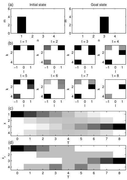
Figure 4: Control for the KL-blocks-world problem with end-cost: example with $m=4,n=4$ and $T=8$. (a) Initial and goal states. (b) Probability of action $p(k^{t},l^{t}|x^{t-1})$ for each time step $t=1\ldots T$. (c) Expected value $\langle x^{t}_{i}\rangle,i=1,\ldots,n$ given the initial position and desired final position and (d) the MAP solution for all times using a gray scale coding with white coding for zero and darker colors coding for higher values.

Figure 4 shows a small example where the planning task is to shift a tower composed of four blocks which initially is at position $1$ to the final position $3$.

To find the KL control we first condition the model both on the initial state and the final state variables by “clamping” all variables $x^{1}$ and $x^{T}$. The KL control solution is obtained by computing for $t=1,\ldots,T$ the marginal $p(k^{t},l^{t}|x^{t-1})$. In this case, we can find the exact solution via the junction tree (JT) algorithm (Lauritzen and Spiegelhalter,, 1988; Mooij,, 2010). The $k^{t},l^{t}$ is obtained by taking the MAP state of $p(k^{t},l^{t}|x^{t-1})$ breaking ties at random, which results in a new state $x_{t}$.

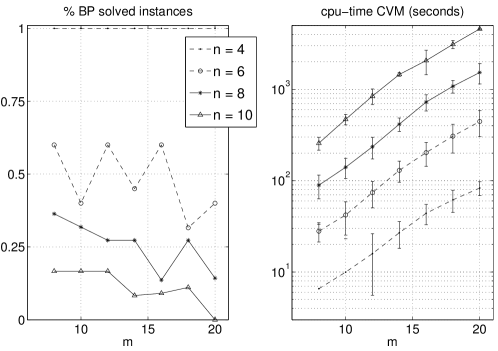
Figure 5: Control for the KL-blocks-world problem with end-cost: results on approximate inference using random initial and goal states. (Left) percent of instances where BP converges for all $t=1:T$ as a function of $m$ for different values of $n$. (Right) CPU-time required for CVM to find a correct plan for different values of $n,m$. $T$ was set to $\lceil\frac{m\cdot n}{4}\rceil$. We run $50$ instances for each pair $(m,n)$.

These probabilities $p(k^{t},l^{t}|x^{t-1})$ are shown in Figure 4b. Notice that the symmetry in the problem is captured in the optimal control, which assigns equal probability when moving the first block to left or right (Figure 4b,c, t=1). Figure 4d shows the strategy resulting from the MAP estimate, which first unpacks the tower at position $1$ leaving all four locations with one block at $t=4$, and then re-builds it again at the goal position $3$.

For larger instances, the JT method is not feasible because of too large tree widths. For instance, to stack 4 blocks on 6 locations within a horizon of 11, the junction tree has a maximal width of 12, requiring about 15 Gbytes of memory. We can nevertheless obtain approximate solutions using different approximate inference methods. In this work, we use the belief propagation algorithm (BP) and a generalization known as the Cluster Variation method (CVM). We briefly summarize the main idea of the CVM method in Appendix C. We use the minimal cluster size, that is, the outer clusters are equal to the interaction potentials $\psi$ as shown in the graphical model Figure 3.

To compute the sequence of actions we follow again a sequential approach. Figure 5 shows results using BP and CVM. For $n=4$, BP converges fast and finds a correct plan for all instances. For larger $n$, BP fails to converge, more or less independently of $m$. Thus, BP can be applied successfully to small instances only. Conversely, CVM is able to find a correct plan in all run instances, although at the cost of more CPU time, as Figure 5 shows. The variance in the CPU error bars is explained by the randomness in the number of actual moves required to solve each instance, which is determined by the initial and goal states.

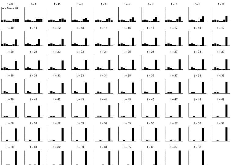
Figure 6: Example of a large block stacking instance without end cost. $n=8,m=40,T=80,\lambda=10$ using CVM.

3.1.2 No goal state and $\lambda>0$: entropy minimization

We now consider the problem without conditioning on $x^{T}$ and $\lambda>0$. Although this may seem counter intuitive, removing the end constraint in fact makes this problem harder, as the number of states that have significant probability for large $t$ is much larger. BP is not able to produce any reliable result for this problem. We applied CVM to a large block stacking problem with $n=8,m=40,T=80$ and $\lambda=10$. We use again the minimal cluster size and the double loop method of Heskes et al., (2003). The results are shown in Figure 6.

The computation time was approximately 1 hour per $t$ iteration and memory use was approximately 27 Mb. This instance was too large to obtain exact results. We conclude that, although the CPU time is large, the CVM method is capable to yield an apparently accurate control solution for this large instance.

4 Multi Agent cooperative game (KL-stag-hunt)

In this section we consider a variant of the stag hunt game, a prototype game of social conflict between personal risk and mutual benefit (Skyrms,, 2004). The original two-player stag hunt game proceeds as follows: there are two hunters and each of them can choose between hunting hare or hunting stag, without knowing in advance the choice of the other hunter. The hunters can catch a hare on their own, giving them a small reward. The stag has a much larger reward, but it requires both hunters to cooperate in catching it.

Table 1: Two-player stag hunt payoff matrix example: rows and columns indicate actions of one and the other player respectively. The payoff describes the reward for each hunter. For instance, if both go for the stag, they both get a reward of $3$. If one hunter goes for the stag and the other for the hare, they get a reward of $0$ and $1$ respectively.

	Stag	Hare
Stag	$\mathbf{3,3}$	$0,1$
Hare	$1,0$	$\mathbf{1,1}$

Table 1 displays a possible payoff matrix for a stag hunt game. It shows that both stag hunting and hare hunting are Nash equilibria, that is, if the other player chooses stag, it is best to choose stag (payoff equilibrium, top-left), and if the other player chooses hare, it is best to choose hare (risk-dominant equilibrium, bottom-right). It is argued that these two possible outcomes makes the game socially more interesting, than for example the prisoners dilemma, which has only one Nash equilibrium. The stag hunt allows for the study of cooperation within social structures (Skyrms,, 1996) and for studying the collaborative behavior of multi-agent systems (Yoshida et al.,, 2008).

We define the KL-stag-hunt game as a multi-agent version of the original stag hunt game where $M$ agents live in a grid of $N$ locations and can move to adjacent locations on the grid. The grid also contains $H$ hares and $S$ stags at certain fixed locations. Two agents can cooperate and catch a stag together with a high payoff $R_{s}$. Catching a stag with more than two agents is also possible, but it does not increase the payoff. The agents can also catch a hare individually, obtaining a lower payoff $R_{h}$. The game is played for a finite time $T$ and at each time-step all the agents perform an action. The optimal strategy is thus to coordinate pairs of agents to go for different stags.

Formally, let $x_{i}^{t}=1,\ldots,N,i=1,\ldots,M,t=1,\ldots,T$ denote the position of agent $i$ at time $t$ on the grid. Also, let $s_{j}=1,\ldots,N,j=1,\ldots,S$, and $h_{k}=1,\ldots,N,k=1,\ldots,H$ denote the positions of the $j$th stag and the $k$th hare respectively. We define the following state dependent reward as:

$$R(x^{t}) =R_{h}\sum_{k=1}^{H}\sum_{i=1}^{M}\delta_{x_{i}^{t},h_{k}}+R_{s}\sum_{j=1}^{S}\mathcal{I}\left\{\left(\sum_{i=1}^{M}x_{i}^{t}=s_{j}\right)>1\right\},$$

where $\mathcal{I}\{\cdot\}$ denotes the indicator function. The first term accounts for the agents located at the position of a hare. The second one accounts for the rewards of the stags, which require that at least two agents to be on the same location of the stag. Note that the reward for a stag is not increased further if more than two agents go for the same stag. Conversely, the reward corresponding to a hare is proportional to the number of agents at its position.

The uncontrolled dynamics factorizes among the agents. It allows an agent to stay on the current position or move to an adjacent position (if possible) with equal probability, thus performing a random walk on the grid. Consider the state variables of an agent in two subsequent time-steps expressed in Cartesian coordinates, $x_{i}^{t}=\langle l,m\rangle,x_{i}^{t+1}=\langle l^{\prime},m^{\prime}\rangle$. We define the following function:

$$\psi_{q}\left(\langle l^{\prime},m^{\prime}\rangle,\langle l,m\rangle\right):=\mathcal{I}\Bigl{\{} \left((l^{\prime}=l)\wedge(m^{\prime}=m)\right)\vee$$

$$\left((l^{\prime}=l-1)\wedge(m^{\prime}=m)\wedge(l>0)\right)\vee$$

$$\left((l^{\prime}=l)\wedge(m^{\prime}=m-1)\wedge(m>0)\right)\vee$$

$$\left((l^{\prime}=l+1)\wedge(m^{\prime}=m)\wedge(l<\sqrt{N})\right)\vee$$

$$\left((l^{\prime}=l)\wedge(m^{\prime}=m+1)\wedge(m<\sqrt{N})\right)\Bigr{\}},$$

that evaluates to one if the agent does not move (first condition), or if it moves left, down, right, up (subsequent conditions) inside the grid boundaries. The uncontrolled dynamics for one agent can be written as conditional probabilities after proper normalization:

$$q\left(x_{i}^{t+1}=\langle l^{\prime},m^{\prime}\rangle|x_{i}^{t}=\langle l,m\rangle\right) =\frac{\psi_{q}(\langle l^{\prime},m^{\prime}\rangle,\langle l,m\rangle)}{\sum_{a,b}{\psi_{q}(\langle a,b\rangle,\langle l,m\rangle)}}.$$

and the joint uncontrolled dynamics become:

$$q(x^{t+1}|x^{t}) =\prod_{i=1}^{M}q(x_{i}^{t+1}|x_{i}^{t}).$$

Since we are interested in the final configuration at end time $T$, we set the state dependent path cost to zero for $t=1,\ldots,T-1$ and to $\exp\left(-\frac{1}{\lambda}R(x^{T})\right)$ for the end time.

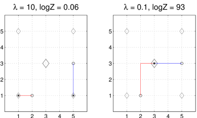
Figure 7: Exact inference KL-stag-hunt: Two hunters in a small grid. There are four hares at each corner of the grid (small diamonds) and one stag in the middle (big diamond). Initial positions of the hunters are denoted by small circles. One hunter is close to a hare and the other is at the same distance of the stag and two hares. Final positions are denoted by asterisks. The optimal paths are drawn in blue and red (Color online). (Left) For $\lambda=10$, the optimal control is risk dominant, and hunters go for the hares. (Right) For $\lambda=0.1$, the payoff dominant control is optimal and hunters cooperate. $N=25,T=4,R_{s}=-10$ and $R_{h}=-2$.

To minimize $C$ in Equation (3), exact inference in the joint space can be done by backward message passing, using the following equations:

$$\beta^{t}({x}^{t}) =\begin{cases}\exp\left(-\displaystyle\frac{1}{\lambda}R({x}^{t})\right)&\text{for $t=T$}\\ \displaystyle\sum_{{x}^{t+1}}q({x}^{t+1}|{x}^{t})\beta({x}^{t+1})&\text{for $t<T$}\end{cases},$$ (17)

and the desired marginal probabilities can be obtained from the $\beta$-messages:

$$p({x}^{t+1}|{x}^{t}) \propto q({x}^{t+1}|{x}^{t})\beta({x}^{t+1}).$$ (18)

To illustrate this game, we consider a small $5\times 5$ grid with two hunters and apply equations (17) and (18). There are four hares at each corner of the grid and one stag in the middle. The initial positions of the hunters are selected in a way that one hunter is close to a hare and the other is at the same distance of the stag and two hares. Starting from the initial fixed state $x^{1}$, we select the next state according to the most probable state from $p(x_{i}^{t+1}|x_{i}^{t})$ until the end time. We break ties randomly. Figure 7 shows one resulting trajectory for two values of $\lambda$.

For high values of $\lambda$ (left plot), each hunter catches one of the hares. In this case, the cost function is dominated by KL term. For small enough values of $\lambda$ (right plot), both hunters cooperate to catch the stag. In this case, the state cost, function $R(x^{T})$, governs the optimal control cost. Thus $\lambda$ can be seen as a parameter that controls whether the optimal strategy is risk dominant or payoff dominant.

Note that computing the exact solution using this procedure becomes infeasible even for small number of agents, since the joint state space scales as $N^{M}$. In the next section, we show a more efficient representation using a factor graph for which approximate inference is tractable.

4.1 Graphical model for the KL-stag-hunt game

The corresponding graphical model of the KL-stag-hunt game is depicted in Figure 8 as a factor graph. Since the uncontrolled dynamics factorizes over the agents, the joint state can be split in different variable nodes.

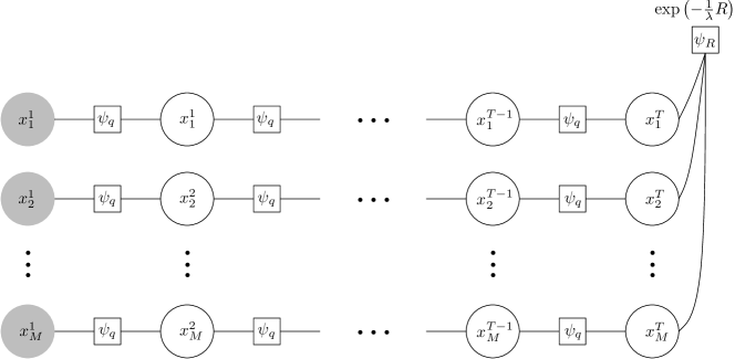
Figure 8: Factor graph representation of the KL-stag-hunt problem. Circles denote variable nodes (states of the agents at a given time-step) and squares denote factor nodes. There are two types of factor nodes: the ones corresponding to the uncontrolled dynamics $\psi_{q}$ and the one corresponding to the state cost $\psi_{R}$. Initial configuration in gray denotes the states “clamped” to an initial given value. Despite being a tree, exact inference and approximate inference are intractable in this model due to the complex factor $\psi_{R}$.

Note that since there is only state cost at the end time, the graphical model becomes a tree. However, the factor node associated to the state cost function $\psi_{R}(x^{T}):=\exp(-\frac{1}{\lambda}R(x^{T}))$ involves all the agent states, which still makes the problem intractable. Even approximate inference algorithms such as BP can not be applied, since messages from $\psi_{R}$ to one of the state variables $x_{i}^{T}$ would require a marginalization involving a sum of $(N-1)^{M}$ terms.

However, we can exploit the particular structure of that factor by decomposing it in smaller factors defined on small sets of (at most three) auxiliary variables of small cardinality. This transformation becomes intuitive once the graphical model representation for the problem is identified. The procedure defines indicator functions for the allowed configurations which are weighted according to the corresponding cost. Figure 9 illustrates the procedure for the case of one stag.

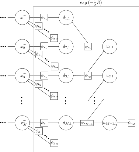
Figure 9: Decomposition of the complex factor $\psi_{R}$ into simple factors involving at most three variables of small cardinality. Each state variable is linked to $H$ factors corresponding to the hares locations. For each stag there is a chain of factors $\psi_{r_{i}},i=1,\ldots,M-1$ which evaluates to one for the allowed configurations and to zero otherwise. Factor $\psi_{r_{M}}$ weights the configuration of having zero, one or more agents being at the stag position (figure shows the case of one stag only).

1. First, we add $H\times M$ factors $\psi_{h_{k}}(x_{i}^{T})$, defined for each hare location $h_{k}$ and each agent variable $x_{i}^{T}$. These factors account for the hare costs:

   $$\psi_{h_{k}}(x_{i}^{T}):= \begin{cases}\exp\left(-\frac{1}{\lambda}R_{h}\right)&\text{if $(x_{i}^{T}=h_{k})$ }\\ 1&\text{otherwise}.\end{cases}$$

2. Second, we add factors $\psi_{s_{j}}(x_{i}^{T},d_{i,j})$ for each stag $j$ defined on each state variable $x_{i}^{T}$ and new introduced binary variables $d_{i,j}=0,1$. These factors evaluate to one when variable $d_{i,j}$ takes the value of a Kronecker $\delta$ of the agent’s state $x_{i}^{T}$ and the position of a stag $s_{j}$, and zero otherwise:

   $$\psi_{s_{j}}(x_{i}^{T},d_{i,j}):=\mathcal{I}\Bigl{\{}(d_{i,j} =\delta_{x_{i}^{T},s_{j}})\Bigr{\}}.$$

3. Third, for each stag, we introduce a chain of factors that involve the binary variables $d_{i,j}$ and additional variables $u_{i,j}=0,1,2$. The new variables $u_{i,j}$ encode whether the stag $j$ has zero, one, or more agents after considering the $(i+1)$th agent. The new factors are:

   $$\psi_{r_{1}}(d_{1,j},d_{2,j},u_{1,j}):=\mathcal{I}\Bigl{\{} \left((d_{1,j}=0)\wedge(d_{2,j}=0)\wedge(u_{1,j}=0)\right)\vee$$

   $$\left((d_{1,j}=1)\wedge(d_{2,j}=1)\wedge(u_{1,j}=2)\right)\vee$$

   $$\left((d_{1,j}\neq d_{2,j})\wedge(u_{1,j}=1)\right)\Bigr{\}}.$$

   $$\psi_{r_{i-1}}(u_{i-1,j},d_{i,j},u_{i,j}):=\mathcal{I}\Bigl{\{} \left((d_{i,j}=0)\wedge(u_{i-1,j}=u_{i,j})\right)\vee$$

   $$\left((d_{i,j}=1)\wedge(u_{i-1,j}=0)\wedge(u_{i,j}=1)\right)\vee$$

   $$\left((d_{i,j}=1)\wedge(u_{i-1,j}=1)\wedge(u_{i,j}=2)\right)\vee$$

   $$\left((d_{i,j}=1)\wedge(u_{i-1,j}=2)\wedge(u_{i,j}=2)\right)\Bigr{\}}.$$

4. Finally, we define factors $\psi_{r_{M}}$ that weight the allowed configurations:

   $$\psi_{r_{M}}(u_{M-1,j}):= \begin{cases}\exp\left(-\frac{1}{\lambda}R_{s}\right)&\text{if $(u_{M-1,j}=2)$ }\\ 1&\text{otherwise}.\end{cases}$$

The original factor can be rewritten marginalizing the auxiliary variables $d_{i,j},u_{i,j}$ over the product of the previous factors $\psi_{s_{j}},\psi_{h_{k}},\psi_{r_{i}}$:

$$\exp\left(-\frac{1}{\lambda}R(x^{T})\right) =\psi_{S}(x^{T})\psi_{H}(x^{T})$$

$$\psi_{S}(x^{T}) :=\prod_{j=1}^{S}\Bigl{[}\sum_{\begin{subarray}{c}d_{1,j},d_{2,j}\\ u_{1,j},u_{M-1,j}\end{subarray}}\left(\psi_{s_{j}}(x_{1}^{T},d_{1,j})\psi_{s_{j}}(x_{2}^{T},d_{2,j})\right)\psi_{r_{1}}(d_{1,j},d_{2,j},u_{1,j})$$

$$\psi_{r_{M}}(u_{M-1,j})\sum_{\begin{subarray}{c}d_{3,j},\ldots,d_{M,j}\\ u_{2,j},\ldots,u_{M,j}\end{subarray}}\prod_{i=3}^{M}\psi_{r_{i-1}}(u_{i-1,j},d_{i,j},u_{i,j})\psi_{s_{j}}(x_{i}^{T},d_{i,j})\Bigr{]}$$

$$\psi_{H}(x^{T}) :=\prod_{k=1}^{H}\psi_{h_{k}}(x_{i}^{T}),$$

where for clarity of notation we have grouped the factors related to the stags and hares in $\psi_{S}(x^{T})$ and $\psi_{H}(x^{T})$, respectively.

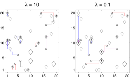
Figure 10: Approximate inference KL-stag-hunt: Control obtained using BP for $M=10$ hunters in a large grid. See Figure 7 for a description of the symbols. (Left) Risk dominant control is obtained for $\lambda=10$, where all hunters go for a hare. (Right) Payoff dominant control is obtained for $\lambda=0.1$. In this case, all hunters cooperate to capture the stags except the ones on the upper-right corner, who are too far away from the stag to reach it in $T=10$ steps. Their optimal choice is to go for a hare. $N=400,S=M/2,R_{s}=-10,H=2M$ and $R_{h}=-2$.

The extended factor graph is tractable since it involves factors of no more than three variables of small cardinality. Note that this transformation can also be applied if additional state costs are incorporated at each time-step $\psi_{R}(x^{t})\neq 0,t=1,\ldots,T$. However, such a representation is not of practical interest, since it complicates the model unnecessarily.

Finally, note that the tree-width of the extended graph still grows fast with the number of agents $M$ because variables $d_{i,j}$ and $u_{i,j}$ are coupled. Thus, exact inference using the JT algorithm is still possible on small instances only.

4.2 Approximate inference of the KL-stag-hunt problem

In this section we analyze large systems for which exact inference is not possible using the JT algorithm. The belief propagation (BP) algorithm is an alternative approximate algorithm that we can run on the previously described extended factor graph.

We use the following setup: for a fixed number of agents $M$, we set the number of stags $H=2M$ and the number of hares $S=\frac{M}{2}$. Their locations, as well as the initial states $x^{1}$ are chosen randomly and non-overlapping. We then construct a factor graph with initial states “clamped” to $x^{1}$ and build instance-dependent factors $\psi_{s_{j}}$ and $\psi_{h_{k}}$. We run BP using sequential updates of the messages. If BP converges in less than $500$ iterations, the optimal trajectories of the agents are computed using the estimated marginals (factor beliefs) for $\psi_{q}(x^{t+1}|x^{t})$ after convergence. Starting from $x^{1}$, we select the next state according to the most probable state from $p_{BP}(x_{i}^{t+1}|x_{i}^{t})$ until the end time. We break ties randomly. We analyze the system as a function of parameter $\lambda$ for a several number of realizations.

The global observed behavior is qualitatively similar to the one of a small system: for $\lambda$ very large, a risk-dominant control is obtained and for $\lambda$ small enough, payoff control dominates. This is behavior is illustrated in Figure 10, where an example for $\lambda=10$ and $\lambda=0.1$ are shown. We can thus conclude that BP provides an efficient and good approximation for large systems where exact inference is not feasible.

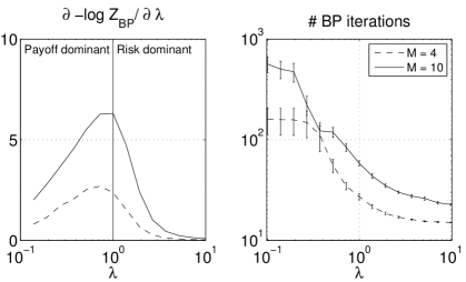
Figure 11: Approximate inference KL-stag-hunt: (Left) Change in the expected cost with respect to $\lambda$ as a function of $\lambda$ for $\langle M=4,N=100\rangle$ and $\langle M=10,N=225\rangle$. The curve becomes sharper and its maximum gets closer to $\lambda=1$ for larger systems, suggesting a phase transition phenomenon between the risk dominant and the payoff dominant regimes. (Right) Number of BP iterations required for convergence as a function of $\lambda$. Results are averages over $20$ runs with random initial states. $R_{s}=-10,R_{h}=-2$ and $T=10$.

To characterize the solutions, we compute the approximated expected cost as in (6), that is $-\log Z_{BP}$. We observe that for large systems that quantity changes abruptly at $\lambda\approx 1$. Qualitatively, the optimal control obtained on the boundary between risk-dominant and payoff-dominant strategies differs maximally between individual instances and strongly depends on the initial configuration. This suggests a phase transition phenomenon typical of complex physical systems, in this case separating the two kind of optimal behaviors, where $\lambda$ plays the role of a “temperature” parameter.

Figure 11 shows this effect. The left plot shows the derivative of the expected approximated cost averaged over $20$ instances. The curve becomes sharper and its maximum gets closer to $\lambda=1$ for larger systems. Error bars of the number of iterations required for convergence is shown on the right. The number of BP iterations quickly increases as we decrease $\lambda$, indicating that the solution for which agents cooperate is more complex to obtain. For $\lambda$ very small, BP may fail to converge after $500$ iterations.

5 Related work

The idea to treat a control problem as an inference problem has a long history. The best known example is the linear quadratic control problem, which is mathematically equivalent to an inference problem and can be solved as a Kalman smoothing problem (Stengel,, 1994). The key insight is that the value function that is iterated in the Bellman equation becomes the (log of the) backward message in the Kalman filter. The exponential relation was generalized in Kappen, (2005) for the non-linear continuous space and time (Gaussian case) and in Todorov, (2007) for a class of discrete problems.

There is a line of research on how to compute optimal action sequences in influence diagrams using the idea of probabilistic inference (Cooper,, 1988; Tatman and Shachter,, 1990; Shachter and Peot,, 1992). Although this technique can be implemented efficiently using the junction tree approach for single decisions, the approach does not generalize in an efficient way to optimal decisions, in the expected-reward sense, in multi-step tasks. The reason is that the order in which one marginalizes and optimizes strongly affects the efficiency of the computation. For a Markov decision process (MDP) there is an efficient solution in terms of the Bellman equation . For a general influence diagram, the marginalization approach as proposed in Cooper, (1988); Tatman and Shachter, (1990); Shachter and Peot, (1992) will result in an intractable optimization problem over $u^{0:T-1}$ that cannot be solved efficiently (using dynamic programming), unless the influence diagram has an MDP structure.

The KL control theory shares similarities with work in reinforcement learning for policy updating. The notion of KL divergence appears naturally in the work of Bagnell and Schneider, (2003) who proposes an information geometric approach to compute the natural policy gradient (for small step sizes). This idea is further developed into an Expectation-Maximization (EM) type algorithm (Dayan and Hinton,, 1997) in recent work (Peters et al.,, 2010; Kober and Peters,, 2011) using a relative entropy term. The KL divergence acts here as a regularization that weights the relative dependence of the new policy on the data observed and the old policy, respectively.

It is interesting to compare the the notion of free energy in continuous-time dynamical systems with Gaussian noise considered in Friston et al., (2009) with the path integral formalism of Kappen, (2005), which is a special case of KL control theory. Friston et al., (2009) advocate the optimization of free energy as a guiding principle to describe behavior of agents. The main difference between the KL control theory and Friston’s free energy principle is that in KL control theory, the KL divergence plays the role of an expected future cost and its optimization yields a (time dependent) optimal control trajectory, whereas Friston’s free energy computes a control that yields a time-independent equilibrium distribution, corresponding to the minimal free energy. Friston’s free energy formulation is obtained as a special case of KL control theory when the dynamics and the reward/cost is time-independent and the horizon time is infinite.

The KL control approach proposed in this paper also bears some relation to the EM approach of Toussaint and Storkey, (2006), who consider the discounted reward case with 0,1 rewards. The posterior can be considered a mixture over times at which rewards are incorporated. For an homogeneous Markov process and time independent costs, the backward message passing can be effectively done in a single chain and not the full mixture distribution needs to be considered. We can compare the EM approach of Toussaint and Storkey, (2006) (TS) and the KL control approach (KL):

• The TS approach is more general than the KL approach, in the sense that the reward considered in TS is an arbitrary function of state and action $R(x,u)$, whereas the reward considered in KL is a sum of a state dependent term $R(x)$ and a KL divergence.

• The KL approach is significantly more efficient than the TS approach. In the TS approach, the backward messages are computed for a fixed policy $\pi$ (E-step), from which an improved policy is computed (M-step). This procedure is iterated until convergence. In the KL approach, the backward messages give the optimal control directly, with no further need for iteration.

• In addition, the KL approach is more efficient than the TS approach for time-dependent problems. Using the TS approach for time-dependent problems makes the computation a factor $T$ more time-consuming than for the time-independent case, since all mixture components must be computed. The complexity of the KL control approach does not depend on whether the problem is time-dependent or not.

• The TS and KL approach optimize with respect to a different quantity. The TS approach writes the state transition $p(y|x)=\sum_{u}p(y|x,u)\pi(u|x)$ and optimizes with respect to $\pi$. The KL approach optimizes the state transition probability $p(y|x)$ directly either as a table or in a parametrized way.

6 Discussion

In this paper, we have shown the equivalence of a class of stochastic optimal control problems to a graphical model inference problem. As a result, exact or approximate inference methods can directly be applied to the intractable stochastic control computation. The class of KL control problems contains interesting special cases such as the continuous non-linear Gaussian stochastic control problems introduced in Kappen, (2005), discrete planning tasks and multi-agent games, as illustrated in this paper.

We notice, that there exist many stochastic control problems that are outside of this class. In the basic formulation of Equation (1), one can construct control problems where the functional form of the controlled dynamics $p^{t}(x^{t+1}|x^{t},u^{t})$ is given as well as the cost of control $R(x^{t},u^{t},x^{t+1},t)$. In general, there may then not exist a $q^{t}(x^{t+1}|x^{t})$ such that Equation (2) holds.

In this paper, we have considered the model based case only. The extension to the model free case would require a sampling based procedure. See Bierkens and Kappen, (2012) for initial work in this direction.

We have demonstrated the effectiveness of approximate inference methods to compute the approximate control in a block stacking task and a multi-agent cooperative task.

For the KL-blocks-world, we have shown that an entropy minimization task is more challenging than stacking blocks at a fixed location (goal state), because the control computation needs to find out where the optimal location is. Standard BP does not give any useful results if no goal state was specified, but apparently good optimal control solutions were obtained using generalized belief propagation (CVM). We found that the marginal computation using CVM is quite difficult compared to other problems that have been studied in the past (Albers et al.,, 2007), in the sense that relatively many inner loop iterations were required for convergence. One can improve the CVM accuracy, if needed, by considering larger clusters (Yedidia et al.,, 2005) as has been demonstrated in other contexts (Albers et al.,, 2006), at the cost of more computational complexity.

We have given evidence that the KL control formulation is particularly attractive for multi-agent problems, where $q$ naturally factorizes over agents and where interaction results from the fact that the reward depends on the state of more than one agent. A first step in this direction was already made in Wiegerinck et al., (2006); van den Broek et al., 2008a . In this case, we have considered the KL-stag-hunt game and shown that BP provides a good approximation and allows to analyze the behavior of large systems, where exact inference is not feasible.

We found that, if the game setting strongly penalizes large deviations from the baseline (random) policy, the coordinated solution is sub-optimal. That means that the optimal solution distributes the agents among the different hares rather than bringing them jointly to the stags (risk-dominant regime). On the contrary, if the agents are not constrained by deviating too much from the baseline policy to maximize $\langle R\rangle$, the coordinated solution becomes optimal (payoff dominant regime). We believe that this is an interesting result, since it provides a explanation of the emergence of cooperation in terms of an effective temperature parameter $\lambda$.

Acknowledgments

We would like to thank anonymous reviewers for helping on improving the manuscript, Kees Albers for making available his sparse CVM code, Joris Mooij for making available the libDAI software and Stijn Tonk for useful discussions. The work was supported in part by the ICIS/BSIK consortium.

Appendix A Boltzmann distribution

Consider the KL divergence between a normalized probability distribution $p(x)$ and some positive function $\psi(x)$:

$$C(p)=\sum_{x}p(x)\log\frac{p(x)}{\psi(x)}$$

$C$ is a function of the distribution $p$. We compute the distribution that minimizes $C$ with respect to $p$ subject to normalization $\sum_{x}p(x)=1$ by adding a Lagrange multiplier:

$$L(p) = C(p)+\beta\left(\sum_{x}p(x)-1\right)$$

$$\frac{dL}{dp(x)} = \log\frac{p(x)}{\psi(x)}+1+\beta$$

Setting the derivative equal to zero yields $p(x)=\psi(x)\exp(-\beta-1)=\psi(x)/Z$, where we have defined $Z=\exp(\beta+1)$. The normalization condition $\sum_{x}p(x)=1$ fixes $Z=\sum_{x}\psi(x)$. Substituting the solution for $p$ in the cost $C$ yields $C=-\log Z$.

Appendix B Relation to continuous path integral model

We write $p(x^{\prime}|x)=\mathcal{N}(x^{\prime}|x+f(x,t)dt+g(x,t)u(x,t)dt,\Xi dt)$ with $\Xi(x,t)=g(x,t)\nu g(x,t)^{T}$ in Equation (9) as

$$p(x^{\prime}|x) ={\cal N}(x^{\prime}|x+f(x,t)dt,\Xi(x,t)dt)\exp\Bigl{(}(\dot{x}-f(x,t))^{T}\Xi^{-1}g(x,t)u(x,t)-$$

$$\qquad\quad\frac{dt}{2}(g(x,t)u(x,t))^{T}\Xi^{-1}g(x,t)u(x,t)\Bigr{)}$$

$$=q(x^{\prime}|x)\exp\left(U(x,x^{\prime},t)dt\right)$$

$$U(x,x^{\prime},t) =(\dot{x}-f(x,t))^{T}\Xi^{-1}g(x,t)u(x,t)-\frac{1}{2}(g(x,t)u(x,t))^{T}\Xi^{-1}g(x,t)u(x,t).$$

with $\dot{x}=(x^{\prime}-x)/dt$.

In order to make the link to Equation (3) we compute

$$\sum_{x^{\prime}}p(x^{\prime}|x)\log\frac{p(x^{\prime}|x)}{q(x^{\prime}|x)} =\sum_{x^{\prime}}p(x^{\prime}|x)U(x,x^{\prime},t)dt$$

$$=\frac{dt}{2}(g(x,t)u(x,t))^{T}\Xi(x,t)^{-1}g(x,t)u(x,t)$$

$$=\frac{dt}{2}u(x,t)^{T}\nu^{-1}u(x,t),$$

where we have made use of the fact that $\sum_{x^{\prime}}p(x^{\prime}|x)x^{\prime}=x+f(x,t)dt+g(x,t)u(x,t)dt$ and $g^{T}\Xi^{-1}g=g^{T}(g^{-1})^{T}\nu^{-1}g^{-1}g=\nu^{-1}$. Therefore,

$$KL(p||q) = \sum_{x^{dt:T}}p(x^{dt:T}|x^{0})\log\frac{p(x^{dt:T}|x^{0})}{q(x^{dt:T}|x^{0})}$$

$$= \sum_{s=0}^{T-dt}\sum_{x^{s}}p(x^{s}|x^{0})\sum_{x^{s+dt}}p(x^{s+dt}|x^{s})U(x^{s},x^{s+dt},s)dt$$

$$= \sum_{s=0}^{T-dt}dt\sum_{x^{s}}p(x^{s}|x^{0})\frac{1}{2}(u(x^{s},s))^{T}\nu^{-1}u(x^{s},s).$$

In the limit of $dt\rightarrow 0$ the KL divergence between $p$ and $q$ becomes

$$KL(p||q) = \left<\int_{0}^{T}dt\frac{1}{2}u(x(s),s)^{T}\nu^{-1}u(x(s),s)\right>$$

in agreement with Equation (10).

Appendix C Cluster Variation Method

In this appendix, we give a brief summary of the CVM method and the double loop approach. For a more complete description see Yedidia et al., (2001); Kappen and Wiegerinck, (2002); Heskes et al., (2003).

The cluster variation method replaces the probability distribution $p(x)$ in the minimization Equation (3) by a large number of (overlapping) probability distributions (clusters), each describing the interaction between a small number of variables.

$$p(x) \approx\{p_{\alpha}(x_{\alpha}),\alpha=1,\ldots\}$$

with each $\alpha$ a subset of the indices $1,\ldots,n$, $x_{\alpha}$ the corresponding subset of variables and $p_{\alpha}$ the probability distribution on $x_{\alpha}$. The set of clusters is denoted by $B$, and must be such that any interaction term $\psi_{\alpha}(x_{\alpha})$, with $\psi(x)=\prod_{\alpha}\psi_{\alpha}(x_{\alpha})$ from Equation (4), is contained in at least one cluster. One denotes the set of all pairwise intersections of clusters in $B$, as well as intersections of intersections by $M$. Figure 12 (left) gives an example of a small directed graphical model, where $B$ consists of 4 clusters and $M$ consists of 5 sub-clusters, Figure 12 (middle).

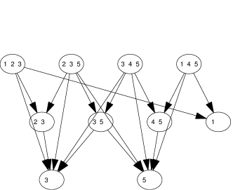
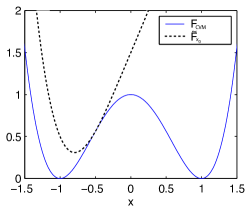
Figure 12: (Left) Example of a small network and a choice of clusters for CVM. (Middle) Intersections of clusters recursively define a set of sub-clusters. (Right) $F_{\mathrm{cvm}}$ is non-convex (blue curve) and is bounded by a convex function $\tilde{F}_{x_{0}}$ (Color online).

The CVM approximates the KL divergence, Equation (3), as

$$C(x^{0},p) \approx F_{\mathsf{cvm}}(\{p_{\alpha}\})$$

$$F_{\mathsf{cvm}}(\{p_{\alpha}\}) =\sum_{\alpha\in B}\sum_{x_{\alpha}}p_{\alpha}(x_{\alpha})\log\frac{p_{\alpha}(x_{\alpha})}{\psi_{\alpha}(x_{\alpha})}+\sum_{\beta\in M}a_{\beta}\sum_{x_{\beta}}p_{\beta}(x_{\beta})\log p_{\beta}(x_{\beta}).$$

$F_{\mathsf{cvm}}$ is minimized with respect to all $\{p_{\alpha}\}$ subject to normalization and consistency constraints:

$$\sum_{x_{\alpha}}p_{\alpha}(x_{\alpha})=1,\qquad p_{\alpha}(x_{\beta})=p_{\beta}(x_{\beta}),\quad\beta\subset\alpha,\qquad p_{\alpha}(x_{\alpha})\geq 0$$

The numbers $a_{\beta}$ are called the Möbius or overcounting numbers. They can be recursively computed from the formula

$$1=\sum_{\alpha\in B\cup M,\alpha\supset\beta}a_{\alpha},\qquad\forall\beta\in B\cup M$$

Since $a_{\alpha}$ can be both positive and negative, $F_{\mathrm{cvm}}$ is not convex. A guaranteed convergent approach to minimize $F_{\mathrm{cvm}}$ is a double loop approach where the outer loop is to upper-bound $F_{\mathrm{cvm}}$ by a convex function $\tilde{F}_{p^{0}}$ that touches at the current cluster solution $p^{0}=\{p^{0}_{\alpha}\}$. Optimizing $\tilde{F}_{p^{0}}(p)$ is a convex problem that can be solved using the dual approach (inner loop) and is guaranteed to decrease $F_{\mathrm{cvm}}$ to a local minimum. The solution $p^{*}(p^{0})$ of this convex sub-problem is guaranteed to decrease $F_{\mathrm{cvm}}$:

$$F_{\mathrm{cvm}}(p^{0})=\tilde{F}_{p^{0}}(p^{0})\geq\tilde{F}_{p^{0}}(p^{*}(p^{0}))\geq F_{\mathrm{cvm}}(p^{*}(p^{0}))$$

Based on $p^{*}(p_{0})$ a new convex upper bound is computed (outer loop). This is called a double loop method. The approach is illustrated in Figure 12 (right).

Alternatively, one can choose to ignore the non-convexity issue. Adding Lagrange multipliers $\lambda$ to enforce the constraints one can minimize with respect to $p=\{p_{\alpha}\}$ and obtain an explicit solution of $p$ in terms of the interactions $\psi$ and the $\lambda$’s. Inserting this solution in the above constraints results in a set of non-linear equations for the $\lambda$’s, which one may attempt to solve by fixed point iteration. It can be shown that these equations are equivalent to the message passing equations of belief propagation. Unlike the above double loop approach, belief propagation does not converge in general, but tends to give a fast and accurate solution for those problems for which it does converge.

References

- Albers et al., (2007) Albers, C. A., Heskes, T., and Kappen, H. J. (2007). Haplotype inference in general pedigrees using the cluster variation method. Genetics, 177(2):1101–1118.
- Albers et al., (2006) Albers, C. A., Leisink, M. A. R., and Kappen, H. J. (2006). The cluster variation method for efficient linkage analysis on extended pedigrees. BMC Bioinformatics, 7(S-1).
- Bagnell and Schneider, (2003) Bagnell, J. A. and Schneider, J. (2003). Covariant policy search. In IJCAI’03: Proceedings of the 18th international joint conference on Artificial intelligence, pages 1019–1024, San Francisco, CA, USA. Morgan Kaufmann.
- Bertsekas and Tsitsiklis, (1996) Bertsekas, D. P. and Tsitsiklis, J. N. (1996). Neuro-Dynamic Programming. Athena Scientific. Belmont. Massachusetts.
- Bierkens and Kappen, (2012) Bierkens, J. and Kappen, B. (2012). Kl-learning: Online solution of Kullback-Leibler control problems. http://arxiv.org/abs/1112.1996.
- Boutilier et al., (1995) Boutilier, C., Dearden, R., and Goldszmidt, M. (1995). Exploiting structure in policy construction. In IJCAI’95: Proceedings of the 14th international joint conference on Artificial intelligence, pages 1104–1111, San Francisco, USA. Morgan Kaufmann.
- Cooper, (1988) Cooper, G. (1988). A method for using belief networks as influence diagrams. In Proceedings of the Workshop on Uncertainty in Artificial Intelligence (UAI’88), pages 55–63.
- da Silva et al., (2009) da Silva, M., Durand, F., and Popović, J. (2009). Linear Bellman combination for control of character animation. ACM Transactions on Graphics, 28(3):82:1–82:10.
- Dayan and Hinton, (1997) Dayan, P. and Hinton, G. E. (1997). Using expectation-maximization for reinforcement learning. Neural Computation, 9(2):271–278.
- Friston et al., (2009) Friston, K. J., Daunizeau, J., and Kiebel, S. J. (2009). Reinforcement learning or active inference? PLoS ONE, 4(7):e6421.
- Heskes et al., (2003) Heskes, T., Albers, K., and Kappen, H. J. (2003). Approximate inference and constrained optimization. In Proceedings of the 19th Conference on Uncertainty in Artificial Intelligence (UAI’03), pages 313–320, Acapulco, Mexico. Morgan Kaufmann.
- Jordan, (1999) Jordan, M. I., editor (1999). Learning in graphical models. MIT Press, Cambridge, MA, USA.
- Kappen, (2005) Kappen, H. J. (2005). Linear theory for control of nonlinear stochastic systems. Physical Review Letters, 95(20):200201.
- Kappen and Wiegerinck, (2002) Kappen, H. J. and Wiegerinck, W. (2002). Novel iteration schemes for the cluster variation method. In Advances in Neural Information Processing Systems 14, pages 415–422. MIT Press, Cambridge, MA.
- Kober and Peters, (2011) Kober, J. and Peters, J. (2011). Policy search for motor primitives in robotics. Machine Learning, 84(1-2):171–203.
- Koller and Parr, (1999) Koller, D. and Parr, R. (1999). Computing factored value functions for policies in structured mdps. In IJCAI ’99: Proceedings of the 16th International Joint Conference on Artificial Intelligence, pages 1332–1339, San Francisco, CA, USA. Morgan Kaufmann.
- Lauritzen and Spiegelhalter, (1988) Lauritzen, S. L. and Spiegelhalter, D. J. (1988). Local computations with probabilities on graphical structures and their application to expert systems. Journal of the Royal Statistical society. Series B-Methodological, 50(2):154–227.
- Mooij, (2010) Mooij, J. M. (2010). libDAI: A free and open source C++ library for discrete approximate inference in graphical models. Journal of Machine Learning Research, 11:2169–2173.
- Murphy et al., (1999) Murphy, K., Weiss, Y., and Jordan, M. (1999). Loopy belief propagation for approximate inference: An empirical study. In Proceedings of the 15th Conference on Uncertainty in Artificial Intelligence (UAI’99), pages 467–47, San Francisco, CA. Morgan Kaufmann.
- Peters et al., (2010) Peters, J., Mülling, K., and Altün, Y. (2010). Relative entropy policy search. In Proceedings of the 24th AAAI Conference on Artificial Intelligence (AAAI 2010), pages 1607–1612. AAAI Press.
- Russell et al., (1996) Russell, S. J., Norvig, P., Candy, J. F., Malik, J. M., and Edwards, D. D. (1996). Artificial intelligence: a modern approach. Prentice-Hall, Inc., Upper Saddle River, NJ, USA.
- Shachter and Peot, (1992) Shachter, R. D. and Peot, M. A. (1992). Decision making using probabilistic inference methods. In Proceedings of the 8th conference on Uncertainty in Artificial Intelligence (UAI’92), pages 276–283, San Francisco, CA, USA. Morgan Kaufmann.
- Skyrms, (1996) Skyrms, B. (1996). Evolution of the Social Contract. Cambridge University Press, Cambridge/New York.
- Skyrms, (2004) Skyrms, B., editor (2004). The Stag Hunt and Evolution of Social Structure. Cambridge University Press, Cambridge, MA, USA.
- Stengel, (1994) Stengel, R. F. (1994). Optimal Control and Estimation. Dover Publications, Inc.
- Tatman and Shachter, (1990) Tatman, J. and Shachter, R. (1990). Dynamic programming and influence diagrams. Systems, Man and Cybernetics, IEEE Transactions on, 20(2):365 –379.
- Theodorou et al., (2009) Theodorou, E. A., Buchli, J., and Schaal, S. (2009). Path integral-based stochastic optimal control for rigid body dynamics. In adaptive dynamic programming and reinforcement learning, 2009. ADPRL ’09. IEEE symposium on, pages 219–225.
- (28) Theodorou, E. A., Buchli, J., and Schaal, S. (2010a). Learning policy improvements with path integrals. In International conference on artificial intelligence and statistics (AISTATS 2010).
- (29) Theodorou, E. A., Buchli, J., and Schaal, S. (2010b). Reinforcement learning of motor skills in high dimensions: A path integral approach. In Proceedings of the International Conference on Robotics and Automation (ICRA 2010), pages 2397–2403. IEEE Press.
- Todorov, (2007) Todorov, E. (2007). Linearly-solvable markov decision problems. In Advances in Neural Information Processing Systems 19, pages 1369–1376. MIT Press, Cambridge, MA.
- Todorov, (2008) Todorov, E. (2008). General duality between optimal control and estimation. In 47th IEEE Conference on Decision and Control, pages 4286–4292.
- Todorov, (2009) Todorov, E. (2009). Efficient computation of optimal actions. Proceedings of the National Academy of Sciences of the United States of America, 106(28):11478–11483.
- Toussaint and Storkey, (2006) Toussaint, M. and Storkey, A. (2006). Probabilistic inference for solving discrete and continuous state Markov Decision Processes. In ICML ’06: Proceedings of the 23rd international conference on Machine learning, pages 945–952, New York, NY, USA. ACM.
- (34) van den Broek, B., Wiegerinck, W., and Kappen, H. J. (2008a). Graphical model inference in optimal control of stochastic multi-agent systems. Journal of Artificial Intelligence Research, 32(1):95–122.
- (35) van den Broek, B., Wiegerinck, W., and Kappen, H. J. (2008b). Optimal control in large stochastic multi-agent systems. Adaptive Agents and Multi-Agent Systems III. Adaptation and Multi-Agent Learning, 4865:15–26.
- Wiegerinck et al., (2006) Wiegerinck, W., van den Broek, B., and Kappen, H. J. (2006). Stochastic optimal control in continuous space-time multi-agent systems. In Proceedings of the 22nd Conference on Uncertainty in Artificial Intelligence (UAI’06), pages 528–535, Arlington, Virginia. AUAI Press.
- Wiegerinck et al., (2007) Wiegerinck, W., van den Broek, B., and Kappen, H. J. (2007). Optimal on-line scheduling in stochastic multi-agent systems in continuous space and time. Proceedings of the 6th international joint conference on Autonomous agents and multiagent systems AAMAS 07, 5:1.
- Yedidia et al., (2001) Yedidia, J., Freeman, W., and Weiss, Y. (2001). Generalized belief propagation. In T.K. Leen, T. D. and Tresp, V., editors, Advances in Neural Information Processing Systems 13, pages 689–995. MIT Press, Cambridge, MA.
- Yedidia et al., (2005) Yedidia, J., Freeman, W., and Weiss, Y. (2005). Constructing free-energy approximations and generalized belief propagation algorithms. Information Theory, IEEE Transactions on, 51(7):2282 – 2312.
- Yoshida et al., (2008) Yoshida, W., Dolan, R. J., and Friston, K. J. (2008). Game theory of mind. PLoS Computational Biology, 4(12):e1000254.