E. V. Votyakov, S. C. Kassinos, X. Albets-Chico Computational Science Laboratory UCY-CompSci, Department of Mechanical and Manufacturing Engineering, University of Cyprus, 75 Kallipoleos, Nicosia 1678, Cyprus

Communicated by

Analytic models of heterogenous magnetic fields for liquid metal flow simulations

Abstract

A physically consistent approach is considered for defining an external magnetic field as needed in computational fluid dynamics problems involving magnetohydrodynamics (MHD). The approach results in simple analytical formulae that can be used in numerical studies where an inhomogeneous magnetic field influences a liquid metal flow. The resulting magnetic field is divergence and curl-free, and contains two components and parameters to vary. As an illustration, the following examples are considered: peakwise, stepwise, shelfwise inhomogeneous magnetic fields, and the field induced by a solenoid. Finally, the impact of the streamwise magnetic field component is shown qualitatively to be significant for rapidly changing fields.

There are few examples in recent history, when things being obvious to particular specialists, remained unexploited by people working in conjugated fields. These include, for instance, the Fast Fourier Transform (FFT), which was originally used by Gauss in 1805 and then several times rediscovered by Lanczos and Danielson in 1942, and Cooley and Tukey in mid-1960s. Another and more specific example is the so-called Savitzky-Golay smoothing filter. The least square method being the base of the filter has been formulated hundred years before experimentalists working with spectra started to use it to treat their data. The paper that popularized this method for the experimentalists is one of the most widely cited papers in the journal Analytical Chemistry.

What is considered in this letter is not as far reaching as the two aforementioned examples, nevertheless, we believe it will help people studying numerically the flow of liquid metals under the influence of an inhomogeneous magnetic field. Also, this letter is complementary to the discussion about magnetic field models given earlier in Votyakov et al. [2008]. The cited work dealt with a 3D distribution of heterogeneous magnetic fields, which are of importance in the case of a magnetic obstacle, while the current letter considers simpler 2D distributions, which are needed, for example, for the proper description of the flow through a fringing magnetic field.

Let us recall shortly the effects of magnetic fields on conducting liquid flows. When the induced magnetic field is negligible, the external magnetic field interacts with the moving liquid and produces the Lorentz force which brakes the flow in the direction of motion, see e.g. Davidson [2001]. This phenomenon is heavily exploited in many practical applications (Davidson [1999]), such as electromagnetic stirring, electromagnetic brakes, and non-contact flow measurements (Thess et al. [2006]).

In reality, one always deals with an inhomogeneous magnetic field because creating a strong and homogeneous magnetic field for experimental needs remains a hard practical challenge. Despite this fact, starting from the pioneering work of Hartmann & Lazarus [1937] many theoreticians love to work mostly with a homogeneous magnetic field. It is clear, that a constant magnetic field is already responsible for main phenomena such as the formation of the Hartmann and parallel layers. Nevertheless, a constant field could not produce the well developed M-shaped velocity profile frequently used for the electromagnetic brake. Due to Kulikovskii [1968], who showed that the flow under the influence of a strong and slowly varying magnetic field can be subdivided in a core and a boundary layer, people started to exploit theoretically inhomogeneous magnetic fields. It was demonstrated that the flow goes parallel to characteristic surfaces, but all the calculations, including the numerical ones, were carried out either by neglecting the second magnetic field component, see, e.g. Sterl [1990], Molokov & Reed [2003b], Molokov & Reed [2003a], Alboussiere [2004], Kumamaru et al. [2004], Kumamaru et al. [2007], Ni et al. [2007] or by employing an especially curvilinear channel Todd [1968] to match boundary conditions. In the case of numerical simulations, there is no particular technical problem preventing the inclusion of the second component of the inhomogeneous magnetic field; nevertheless this has not been done. A probable explanation for this is the absence of suitable and analytically simple models to define an inhomogeneous magnetic field. Therefore, there is the need for convenient formulae that could allow us to do so, and the goal of the paper is to provide a simple method that can be used in numerical studies so that both components can be varied in a consistent way. At the end of the paper we discuss briefly the legitimacy of omitting the streamwise component of the magnetic field, and show that in some cases this might have been done due to large aspect ratios.

It is worth to note that there are examples where correct expressions for a heterogenous magnetic field have been used for MHD flow simulations. These are 2D numerical papers by Cuevas et al. [2006a, b] who correctly applied formulae taken from the book of McCaig [1977]. Those 2D simulations hired only the transverse component of the magnetic field while the second component played no role. More sophisticated 3D cases are given in Votyakov et al. [2007, 2008], where all three components of the magnetic field are taken into account.

The necessity to have at least two nonzero components of the inhomogeneous magnetic field (hereafter denoted as MF) follows directly from the requirement that, in the flow region, an externally applied field must be simultaneously divergence-free $\nabla\cdot\bf{B}=0$ and curl-free $\nabla\times\bf{B}=0$. Thus, if the transverse MF component varies along the streamwise coordinate, the streamwise MF component must vary consistently along the transverse coordinate. (The spanwise component can be neglected without violation of the physical correctness, when the magnetic field is two dimensional.) A vector field that is simultaneously divergence-free and curl-free is known as a Laplace vector field and it can be defined in terms of the gradient of any function $\eta$ which is harmonic in the flow region, $\bf{B}=-\nabla\eta$, $\Delta\eta=0$. This function $\eta$ is called the magnetic scalar potential. Although this is the most general approach, see e.g. McCaig [1977], it is not quite convenient because boundary conditions for $\eta$ must be defined for each specific case. However, what we need is a magnetic field which either vanishes or goes monotonically onto a constant level far away from the central point where the intensity of the field is maximal. So, among all the possible harmonic functions, we may select those that do not vary at far distances, and this forms the basis for the proposed methodology.

A simple, flexible, and physically consistent way to define an inhomogeneous MF for parametric numerical needs is based on the magnetic field induced by a single magnetic dipole. This field is local in space and its magnetic scalar potential, which below is called ”an elementary potential”, belongs to harmonic functions. The whole magnetic field is the sum of local fields from the single magnetic dipoles, therefore, the whole magnetic field can also be represented as the gradient of a scalar function, i.e. as a whole scalar potential. In other words, the single magnetic dipole can be taken as an elementary unit in the appropriate spatial distribution of magnetic sources. The field ${\bf B^{\prime}}({\bf r,r^{\prime}})$ created at ${\bf r}=(x,y,z)$ by a single dipole ${\bf m}=(0,0,m)$ located at ${\bf r^{\prime}}=(x^{\prime},y^{\prime},z^{\prime})$ is given by Jackson [1999]:

$${\bf B^{\prime}}({\bf r,r^{\prime}})=\nabla\times\left(\nabla\frac{1}{|{\bf r-r^{\prime}}|}\times{\bf m}\right)=({\bf m}\cdot\nabla)\left(\nabla\frac{1}{|{\bf r}-{\bf r^{\prime}}|}\right)=m\nabla\frac{\partial}{\partial z}\left(\frac{1}{|\bf{r}-\bf{r^{\prime}}|}\right),$$ (1)

where we have used few vector identities and omitted the constant $\mu_{0}/(4\pi)$. Let the dipoles be distributed in the finite region $\Omega$ outside of the flow. Then, it is easy to see that the elementary $\eta^{\prime}$ and the whole scalar potential $\eta$ are given by:

$$\eta^{\prime}(x,y,z,x^{\prime},z^{\prime},z^{\prime}) = -m\frac{\partial}{\partial z}\left(\frac{1}{|\bf{r}-\bf{r^{\prime}}|}\right)=\frac{m(z-z^{\prime})}{|\bf{r}-\bf{r^{\prime}}|^{3}},$$ (2)

$$\eta(x,y,z) = \int_{\Omega}\eta^{\prime}(x,y,z,x^{\prime},z^{\prime},z^{\prime})dx^{\prime}dy^{\prime}dz^{\prime}=\int_{\Omega}\frac{m(z-z^{\prime})}{|\bf{r}-\bf{r^{\prime}}|^{3}}dx^{\prime}dy^{\prime}dz^{\prime}\,.$$ (3)

This is the simplest model of a permanent magnet occupying the region $\Omega$ with the constant magnetic dipole distribution $m$. By taking various $\Omega$, one can define any desired inhomogeneous MF for parametric numerical needs and mimic roughly various magnetic systems. Below in Fig.1 we give few simple examples of two-dimensional, i.e. $B_{y}(x,y,z)=0$, fields constructed in this way to represent typical magnetic field configurations. Everywhere, $x$ (left to right) is streamwise, $y$ - spanwise (perpendicular to the plane of Fig. 1), and $z$ (down to up) is transverse coordinate.

Here it is worth noting that any two-dimensional field can be conveniently expressed through a complex representation. Introducing the variable $\zeta=x+iz$, and its conjugate $\zeta^{*}=x-iz$, one may define a complex function

$$\beta(\zeta)=B_{x}+i\,B_{z},$$ (4)

where $B_{x}=\rm{Re}(\beta)$, and $B_{z}=\rm{Im}(\beta)$. The function $\beta(\zeta)$ is given below as well.

Linear chain of equal dipoles oriented parallel to $z$ direction and infinitely extended in the $y$ direction at $(x_{0},z_{0})$, $\Omega=\{x=x_{0},-\infty\leq y\leq\infty,z=z_{0}\}$:

$$\begin{split}\eta(x,y,z)&=\int_{-\infty}^{\infty}\int_{-\infty}^{\infty}\int_{-\infty}^{\infty}\frac{m(z-z^{\prime})\delta(x^{\prime}-x_{0})\delta(z^{\prime}-z_{0})dx^{\prime}dy^{\prime}dz^{\prime}}{((x-x^{\prime})^{2}+(y-y^{\prime})^{2}+(z-z^{\prime})^{2})^{3/2}}\\ &=\frac{2m(z-z_{0})}{(x-x_{0})^{2}+(z-z_{0})^{2}}=\frac{2m\cos\varphi}{l}\end{split}$$ (5)

$$B_{x}(x,y,z) =-\frac{\partial\eta(x,y,z)}{\partial x}=\frac{4m(x-x_{0})(z-z_{0})}{\left((x-x_{0})^{2}+(z-z_{0})^{2}\right)^{2}}=\frac{2m\sin 2\varphi}{l^{2}},$$ (6)

$$B_{z}(x,y,z) =-\frac{\partial\eta(x,y,z)}{\partial z}=\frac{2\,m\left((z-z_{0})^{2}-(x-x_{0})^{2}\right)}{\left((x-x_{0})^{2}+(z-z_{0})^{2}\right)^{2}}=-\frac{2m\cos 2\varphi}{l^{2}},$$ (7)

$$\beta(\zeta) =2\,m\,i\frac{(\zeta-\zeta_{0})^{2}}{|\zeta-\zeta_{0}|^{4}}=\frac{2\,m\,i}{(\zeta^{*}-\zeta^{*}_{0})^{2}},$$ (8)

here, $l$ and $\varphi$ define the cylindrical coordinate system $(x-x_{0})=l\cos\varphi,\quad(z-z_{0})=l\sin\varphi$, and the angle $\varphi$ is taken as counter-clockwise. Fig.1a shows an example of the magnetic field induced by two symmetrically located chains of dipoles in the rectangular channel.

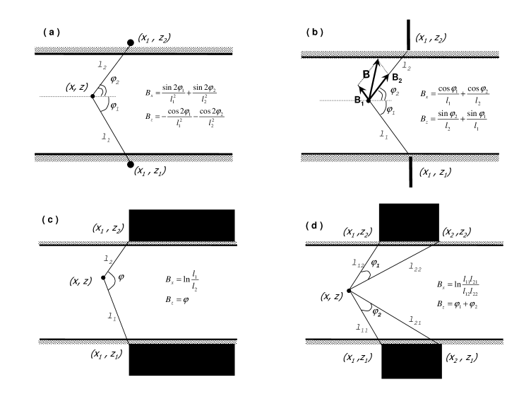
Figure 1: Inhomogeneous magnetic field created in the duct by linear chains of identical dipoles($a$), two identical sheets dipoles($b$), half space ($c$), and two magnets ($d$). Angles $\varphi$, $\varphi_{1}$, $\varphi_{2}$ must be taken as counter-clockwise, $m$ is taken equal one. Also, ($b$) shows a geometrical construction to find the final magnetic field, see Eq. 10-11

The sheet of magnetic dipoles, Fig.1$b$, is made by stacking the linear chains described above along the $z$ axis, $\Omega=\{x=x_{0},-\infty\leq y\leq\infty,z_{0}\leq z\leq\infty\}$. Therefore for this case, the magnetic field is obtained by an integration of Eqs. (5-8) over $z$, from $z_{0}$ to infinity:

$$\eta(x,y,z) =-m\ln\left((x-x_{0})^{2}+(z-z_{0})^{2}\right)=2m\ln\frac{1}{l}$$ (9)

$$B_{x}(x,y,z) =\frac{2m(x-x_{0})}{(x-x_{0})^{2}+(z-z_{0})^{2}}=\frac{2m\cos\varphi}{l},$$ (10)

$$B_{z}(x,y,z) =\frac{2m(z-z_{0})}{(x-x_{0})^{2}+(z-z_{0})^{2}}=\frac{2m\sin\varphi}{l},$$ (11)

$$\beta(\zeta) =2\,m\frac{\zeta-\zeta_{0}}{|\zeta-\zeta_{0}|^{2}}=\frac{2\,m}{(\zeta^{*}-\zeta^{*}_{0})}.$$ (12)

This particular magnetic dipole configuration allows the construction of the final magnetic field through a clear geometrical interpretation. Fig. 1$b$ shows this construction: the vector $\bf B_{1}$ is the field created by the lower sheet and is directed along the $\bf(r-r_{1})$, while its length is inverse to $l_{1}$; on the other hand, vector $\bf B_{2}$ is the field created by the upper sheet, it points along the $\bf(r-r_{2})$ with a length inversely proportional to $l_{2}$; the vector sum ${\bf B=B_{1}+B_{2}}$ is the final magnetic field in the duct.

The stepwise magnetic field can be obtained by the integration of the sheet fields from the edge point $x_{1}$ up to infinity, ($\Omega=\{x_{1}\leq x\leq\infty,-\infty\leq y\leq\infty,-\infty\leq z\leq z_{1}\bigcup z_{2}\leq z\leq\infty\})$, see these coordinates in Fig. 1c). To exclude the divergence for $B_{x}$ at $x\rightarrow\infty$, we add a second magnetic half-space, then:

$$B_{x}(x,y,z) =m\,\ln\frac{(x-x_{1})^{2}+(z-z_{1})^{2}}{(x-x_{1})^{2}+(z-z_{2})^{2}}=2\,m\ln\frac{l_{1}}{l_{2}}$$ (13)

$$B_{z}(x,y,z) =2\,m\left(\arctan\frac{z-z_{1}}{x-x_{1}}+\arctan\frac{z-z_{2}}{x-x_{1}}\right)=2\,m\,\varphi,$$ (14)

$$\beta(\zeta) =2\,m\ln\frac{\zeta-\zeta_{1}}{\zeta-\zeta_{2}}.$$ (15)

This, so called fringing, magnetic field is a candidate configuration for the proper study of the transformation of the Poiseuille velocity profile to the Hartmann one, and the dependence of a transition length as a function of $Re$ and $Ha$. To our knowledge there are no papers to date that apply a physically correct fringing magnetic field in numerical simulations, even though this field is one of the most heavily studied in liquid metal flows, see Molokov & Reed [2003b], Alboussiere [2004], Kumamaru et al. [2004], Kumamaru et al. [2007], Ni et al. [2007]. Below we derive qualitatively what is the effect of the streamwise magnetic component of the fringing field on the transverse pressure distribution in the duct.

The shelfwise magnetic field, created by a homogenous dipole distribution, is obtained if $\Omega$ is restricted in the $x$ direction ($\Omega~{}=~{}\{x_{1}\leq x\leq x_{2},-\infty\leq y\leq\infty,-\infty\leq z\leq z_{1}\cup z_{2}\leq z\leq\infty\}$). Fig. 1d shows this configuration:

$$\begin{split}B_{x}(x,y,z)&=\frac{m}{2}\ln\frac{l_{11}l_{21}}{l_{12}l_{22}}\\ &=\frac{m}{2}\ln\frac{((x-x_{1})^{2}+(z-z_{1})^{2})((x-x_{2})^{2}+(z-z_{1})^{2})}{((x-x_{1})^{2}+(z-z_{2})^{2})((x-x_{2})^{2}+(z+z_{2})^{2})}\end{split}$$ (16)

$$\begin{split}B_{z}(x,y,z)&=m(\varphi_{1}+\varphi_{2})\\ &=m\left(\arctan\frac{z-z_{2}}{x-x_{1}}-\arctan\frac{z-z_{2}}{x-x_{2}}+\arctan\frac{z_{1}-z}{x-x_{1}}-\arctan\frac{z_{1}-z}{x-x_{2}}\right),\end{split}$$ (17)

$$\beta(\zeta) =m\ln\frac{(\zeta-\zeta_{11})(\zeta-\zeta_{21})}{(\zeta-\zeta_{12})(\zeta-\zeta_{22})}.$$ (18)

By varying the parameters $x_{1},x_{2},z_{1},z_{2}$, one can regulate the width of the central region and the upward (outward) gradient of the magnetic field.

In above examples, the $z$ integration is taken over two half-open regions $\{-\infty\leq z\leq z_{1}\bigcup z_{2}\leq z\leq\infty\}$. It is easy to perform the integration up to a finite z-value instead of infinity, however, this case is not considered in order to simplify formulae and keep the essence of the method. Moreover, in practice, a magnetic system is supported by the yoke made of soft iron. This effectively means a closure for the lines of the magnetic field coming from the external side of the magnet (where the internal side is adjoined to the duct), therefore, the upper limit of the integration can be safely set as infinity.

Up to now, we have learned how to define an external magnetic field by means of magnetic dipoles. Usage of magnetic dipole language dictates the following scaling behavior for the magnetic field far from the central point: $l^{-3}$ for a single dipole, $l^{-2}$ for a linear chain, $l^{-1}$ for a sheet, and $\ln l$ for a massive body, where $l$ is a distance from the object, (see Fig. 1). It’s possible to make this slope even more smooth, i.e. $l\ln l$, if, instead of the magnetic domain, we take a cross section of constant current density $j$, taken everywhere equal to one. Physically, it means that instead of using the permanent magnet considered before, we shall deal with a conducting cable carrying the electric current of homogenous density. The easiest way to understand how we could develop mathematically the cable from the magnet is described next.

First, we may present the magnetic domain as a non-conducting cross-section enabling surface currents only. Schematically, it is shown in Fig. 2$a$ by taking six magnetic dipoles together in close contact: all the internal currents from the adjoining magnetic dipoles are mutually compensated because they run in opposite directions, therefore, the only non-compensated electric currents are located on the bordering surfaces. The next step is to extend the surface current obtained above, in such a way that it flows through a finite rectangular region, i.e. through cable of rectangular cross-section. The configuration of the rectangular conductor is shown in Fig. 2$b$., where the corners are $(x_{k},z_{l}),\mbox{ }k,l=1,2$ (the diagonal cross in Fig. 2$b$ denotes electric current running in the direction perpendicular the plane of the figure). Such a cable can be represented as a part of the top (cables II and IV) and bottom (cables I and III) solenoids assembled around the channel, see Fig. 2$c$.

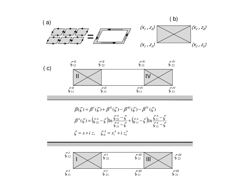
Figure 2: Scheme showing an equivalence of the magnetic domain and a body with surface currents ($a$), notations used to write down magnetic field from a cable ($b$), scheme of two primitive solenoids located under and above duct($c$), the cables are supposed to encircle at $y=\pm\infty$, see text and Eq. (19, 20)

To derive the magnetic field produced by the aforesaid primitive solenoids, we note that the shelfwise magnetic system shown in Fig.1$d$, Eqs. (16)-(18), is equivalent to the solenoids having infinitely thin cables located at $x=x_{1}$ and $x=x_{2}$ because all internal currents in this system are mutually compensated in the way explained above by Fig. 2$a$. Therefore, if one integrates $\beta(\zeta)$ given by Eq. (18) over the complex variable $\zeta=x+iz$ confined by cable’s corners shown in Fig. 2$b$, then one obtains the following complex function for the individual cable $A$:

$$\beta^{A}(\zeta) = (\zeta^{A}_{22}-\zeta)\ln\frac{\zeta^{A}_{22}-\zeta}{\zeta^{A}_{21}-\zeta}+(\zeta^{A}_{11}-\zeta)\ln\frac{\zeta^{A}_{11}-\zeta}{\zeta^{A}_{12}-\zeta},$$ (19)

where $A=I,II,III,IV$ should be taken for different cables, and $\zeta^{A}_{k,l}=x_{k}^{A}+iz_{l}^{A},\mbox{ }k,l=1,2$ are for the coordinates of the corners of cable $A$, see Fig. 2$c$. The final complex function for the top and bottom solenoids is obtained as a superposition of terms coming from four cables:

$$\beta(\zeta) = \beta^{I}(\zeta)+\beta^{II}(\zeta)-\beta^{III}(\zeta)-\beta^{IV}(\zeta),$$ (20)

where terms from cables I and II are positive and for cables III and IV are negative because the direction of the electric current in cables I and II is opposite to the direction of current in cables III and IV. The final $\beta(\zeta)$, Eq. 20, is the linear superposition of the products of logarithmic and rational functions depending on a complex variable $\zeta=x+i\,z$. Then, by means of algebraic transformations, the obtained $\beta(\zeta)$ should be presented as a sum of its real and imaginary parts (cf. Eq. 4), so that $B_{x}=\rm{Re}[\beta(\zeta)]$ and $B_{z}=\rm{Im}[\beta(\zeta)]$. Although they have been obtained, the mathematical expressions for $B_{x}$ and $B_{z}$ are quite cumbersome and for the sake of brevity they are not reported here.

To conclude, we show briefly what is the impact of the streamwise field component on a liquid metal flow in the case of the fringing magnetic field. As it is widely accepted, inertia and viscosity vanish in the core of a duct MHD flow, therefore, the pressure distribution, $p$, is governed in the core by the Lorentz force, $\nabla p={\bf j}\times{\bf B}$, where ${\bf j}$ are the induced electric currents. This means that $\nabla p$ is perpendicular to $\bf B$, i.e. the pressure contour lines are matched with magnetic field lines. Thus, if one employs the transverse field component only, the pressure contour lines are straightened in the transverse direction, while they must be curved in accordance with the curvature of the external magnetic field, see Fig. 3.

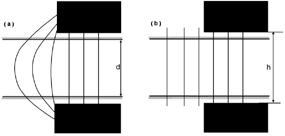
Figure 3: Pressure contour lines matching magnetic field lines with ($a$) and without ($b$) streamwise magnetic field component.

Curvature of the magnetic field lines depends on the aspect ratio $d/h$, where $d$ ($h$) is the height of the duct (magnetic gap). As $d/h$ decreases, the curvature vanishes, however the inward gradient of the magnetic field decreases as well. Hence, in order to study the effects of a rapidly varying fringing magnetic field, the streamwise field component must be taken into account necessarily.

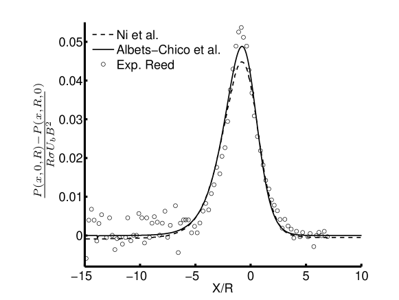
Figure 4: Dimensionless transverse pressure difference for the so called Benchmark fringing magnetic field case. Comparison is given for experimental results (Reed et al. [1987], circles), 3D numerics with a non-consistent fringing magnetic field (dashed, Ni et al. [2007]), and 3D numerics with a consistent magnetic field (solid, Albets-Chico et al. [2009]) The results are clearly improved when the consistent magnetic field is considered.

As a paradigmatic example, the well-known nuclear fusion benchmark fringing magnetic field case based on the experiment of Reed et al. [1987] ($Ha=6569$, $N=10824$, $c=0.027$) has been recently studied using a complete numerical resolution of the Navier-Stokes equations by Ni et al. [2007]. Details regarding the shape of the fringing magnetic field, geometry and boundary conditions for this case are clearly exposed in both the experimental Reed et al. [1987] and the numerical Ni et al. [2007] works.

Ni et al. [2007] presented 3D numerical results in very good agreement with the experimental data although a non negligible under-prediction ($\approx 16\%$) of the peak transverse pressure difference was also reported. Ni et al. applied a tanh-based fitting function to approximate the main component of the experimental magnetic field, while the additional components were neglected. More recently, Albets-Chico et al. [2009] have also addressed this case by means of a complete numerical resolution of the governing equations (considering a quasi-static approximation for the induced magnetic field) when using a nodal-based non-structured finite-volume code. Details regarding the form of the addressed Navier-Stokes equations and the assumed simplifications can be found in Ni et al. [2007], as both works have employed essentially the same methodology. Additionally, Albets-Chico et al. have analyzed the effect of the consistency of the magnetic field while developing a mathematical technique to generate consistent magnetic fields from experimental fits. Further, details will be available soon in Albets-Chico et al. [2009].

Fig. 4 presents the effect of the consistency of the magnetic field in the transverse pressure difference results. When using a consistent magnetic field, the under-prediction for the peak is reduced to approximately 9%, which clearly demonstrates how the consistency of the magnetic field plays an important role related to the transverse pressure difference in such a case. It is interesting to note that Albets-Chico et al. obtained a perfect agreement with Ni et al. [2007] results when using a non-consistent magnetic field (based on the same tanh-based fitting function as the one used in Ni et al.). Finally, Albets-Chico et al. explain the still remaining under-prediction in terms of the experimental results in the nature (slope and order of accuracy) of the fitting function.