Quadrupole Oscillations in Bose-Fermi Mixtures of Ultracold Atomic Gases made of Yb atoms
in the Time-Dependent Gross-Pitaevskii and Vlasov equations

Abstract

We study quadrupole collective oscillations in the bose-fermi mixtures of ultracold atomic gases of Yb isotopes, which are realized by Kyoto group. Three kinds of combinations are chosen, ¹⁷⁰Yb$-^{171}$Yb , ¹⁷⁰Yb$-^{173}$Yb and ¹⁷⁴Yb$-^{173}$Yb , where boson-fermion interactions are weakly repulsive, strongly attractive and strongly repulsive respectively. Collective oscillations in these mixtures are calculated in a dynamical time-evolution approach formulated with the time-dependent Gross-Pitaevskii and the Vlasov equations. The boson oscillations are shown to have one collective mode, and the fermions are shown to have the boson-forced and two intrinsic modes, which correspond to the inside- and outside-fermion oscillations for the boson-distributed regions. In the case of the weak boson-fermion interactions, the dynamical calculations are shown to be consistent with the results obtained in the small amplitude approximations as the random phase approximation in early stage of oscillation, but, in later stage, these two approaches are shown to give the different results. Also, in the case of the strong boson-fermion interactions, discrepancies appear in early stage of oscillation. We also analyze these differences in two approaches, and show that they originated in the change of the fermion distributions through oscillation.

I Introduction

Over the last several years, there have been significant progresses in ultracold atomic gas physics GPS : Bose-Einstein condensates (BEC) nobel ; Dalfovo ; becth ; Andersen , two boson mixtures B-B , Fermi-degenerate atomic gases ferG , and Bose-Fermi (BF) mixtures Schreck ; BferM ; Modugno , and so on. In particular, the BF mixtures attract physical interests as a typical example where particles obeying different quantum statistics are intermingled. In the study of this system, we have a big opportunity to obtain a lot of new knowledge on quantum many-body systems because we can make a variety of mixtures with atomic specie combinations and can control the atomic interactions using the Feshbach-resonance method Fesh . Theoretical studies of the BF mixtures have been done on static properties Molmer ; Amoruso ; MOSY ; Bijlsma ; Vichi ; Vichi1 , the phase structures and separation Nygaard ; Yi ; Viverit ; Capuzzi02 , induced instabilities by the attractive interactions MSY1 ; Roth ; Capuzzi03 , and the collective excitations MSY ; Minguzzi ; zeros ; Yip ; sogo ; miyakawa ; Liu ; tomoBF ; monoEX ; tbDPL ; scalTF ; scalTF2 .

One of important diagnostic signals of many-particle systems is the collective excitations because of their sensitivity on the inter-atomic interactions and the ground- and excited-state structures. Theoretically, collective motions are usually studied in the random phase approximation (RPA) zeros ; sogo or its approximate methods: the sum-rule miyakawa ; MSY or the scaling Liu ; scal ; scalDP ; scalTF ; scalTF2 methods.

In the previous papers, we calculated time-evolution of the BF mixtures directly with solving the time-dependent Gross-Pitaevskii (TDGP) and the Vlasov equations, and studied their monopole tomoBF ; monoEX and dipole tbDPL oscillations; the results are largely consistent with the RPA calculations sogo , but show different behaviors in some aspects: for example, the rapid damping at zero temperature ($T=0$).

In the BF mixtures at $T=0$, the condensed bosons occupy one single-particle state, and the fermions distribute in a wide range of single-particle states. Thus the boson oscillation has only one collective mode in spectrum with no strong damping chevy ; tohyama ; on the other hand, various collective modes appear in the fermion collective oscillation generally. The RPA calculations ColBTh can explain the experimental results on the frequencies of collective motionsColEx . Especially, in the fermion oscillation of the BF mixtures, two regions of the fermi gas, inside and outside of the boson distributions, oscillate with different frequencies, and their interference gives the beat and damping phenomena, which are clearly shown in the time-evolution approach; on the other hand, the boson oscillation become monotonous tomoBF ; tbDPL .

In the time-evolution approach, the intrinsic frequencies of the oscillation modes can be obtained from the Fourier transform of the time-dependence of the collective coordinates. In the dipole oscillation of the fermion components, we have really confirmed the existence of the two intrinsic modes corresponding to the inside- and outside motions and one forced-oscillation mode caused by the boson oscillation tbDPL . In the early stage of the oscillation, these intrinsic frequencies obtained in the time-evolution approach are consistent with the RPA calculation, but, in the later stage, the two calculations show different results tomoBF ; the difference is originated in the distribution changes of the density and the velocity in time-developments, which appears in the time-evolution approach but not in harmonic approximations like the RPA calculations. In actual experiments, the oscillation amplitude is not so small ColEx that the results obtained in the time-dependent approach should be more reliable in comparison with experiments.

In this paper, we consider the BF mixtures of the Yb isotopes, which have some particular properties; the Yb consists of many kinds of isotopes, five bosons (^{168,170,172,174,176}Yb) and two fermions (^171,173Yb), which give a variety of combinations in the BF mixtures. Experimental researches on the trapped atomic gases of the Yb isotopes are being performed actively by the group of Kyoto university; the BEC Takasu and the Fermi-degeneracy Fukuhara1 have been performed. The scattering lengths for the boson-fermion interactions have been obtained experimentally by the group Fukuhara1 ; Fukuhara2 ; Kitagawa , and the observation of the ground state properties and the collective oscillations of the BF mixtures is now under progressing.

In this paper, we discuss the quadrupole oscillations of the BF mixtures of Yb isotopes in the time-evolution approach, where the time evolution of the condensed-boson wave function and the fermion phase-space distribution function are obtained from the solutions of the TDGP and Vlasov equations, respectively. In the next section, we give the formulation of the transport model to calculate the time evolution. In Sec. III, the numerical results on the quadrupole oscillations are shown with their physical properties for three kinds of BF mixtures, ¹⁷⁰Yb$-^{171}$Yb , ¹⁷⁰Yb$-^{173}$Yb and ¹⁷⁴Yb$-^{173}$Yb . Sec. IV is for summary.

II Time-Dependent Gross-Pitaevskii and Vlasov Equations

In this section, we briefly explain the time-evolution approach to calculate collective oscillations of the BF mixture. Let’s consider the system of the coexistent dilute gases of one bosonic and one-component fermionic atoms at $T=0$, which is trapped in the axially-symmetric potential with respect to the $z$-axis. The zero-range boson-boson and boson-fermion interactions are assumed, and no fermion-fermion interaction exists in the system. Then the hamiltonian of the system is

$${\tilde{H}}=\int d^{3}{q}~{}\Bigg{[} - \frac{\hbar^{2}}{2M_{B}}{\tilde{\phi}}^{\dagger}(\mbox{\boldmath$q$})\nabla^{2}_{q}{\tilde{\phi}}(\mbox{\boldmath$q$})+\frac{1}{2}M_{B}\Omega_{B}^{2}(\mbox{\boldmath$q$}_{T}^{2}+\kappa_{L}^{2}q_{L}^{2}){\tilde{\phi}}^{\dagger}(\mbox{\boldmath$q$}){\tilde{\phi}}(\mbox{\boldmath$q$})$$ (1)

$$+ \frac{2\pi\hbar^{2}a_{BB}}{M_{B}}\{{\tilde{\phi}}^{\dagger}(\mbox{\boldmath$q$}){\tilde{\phi}}(\mbox{\boldmath$q$})\}^{2}$$

$$- \frac{\hbar^{2}}{2M_{f}}{\tilde{\psi}}^{\dagger}(\mbox{\boldmath$q$})\nabla_{q}^{2}{\tilde{\psi}}(\mbox{\boldmath$q$})+\frac{1}{2}M_{f}\Omega_{F}^{2}(\mbox{\boldmath$q$}_{T}^{2}+\kappa_{L}^{2}q_{L}^{2}){\tilde{\psi}}^{\dagger}(\mbox{\boldmath$q$}){\tilde{\psi}}(\mbox{\boldmath$q$})$$

$$+ \frac{2\pi\hbar^{2}a_{BF}(M_{B}+M_{F})}{M_{B}M_{F}}{\tilde{\phi}}^{\dagger}(\mbox{\boldmath$q$}){\tilde{\phi}}(\mbox{\boldmath$q$}){\tilde{\psi}}^{\dagger}(\mbox{\boldmath$q$}){\tilde{\psi}}(\mbox{\boldmath$q$})\Bigg{]},$$

where ${\tilde{\phi}}$ and ${\tilde{\psi}}$ are boson and fermion fields, respectively, $M_{B,F}$ are the boson and fermion masses, $\Omega_{B,F}$ are the transverse frequencies of the trapping potentials for the boson and the fermion, and $a_{BB,BF}$ are the boson-boson and boson-fermion $s$-wave scattering lengths. The transverse and longitudinal components of the spatial coordinate are described by $\mbox{\boldmath$q$}\equiv(\mbox{\boldmath$q$}_{T},q_{L})$, and $\kappa_{L}$ is the longitudinal-to-transverse frequency ratio of the trapping potentials; in this paper, we assume the same ratio for the bosons and fermions.

To reduce the parameters, we rewrite Eq. (1) with the dimensionless variables; the scaled spatial coordinates $R_{B}=(\hbar/M_{B}\Omega_{B})^{1/2}$ and the scaled boson/fermion fields $\phi=R_{B}^{-1/3}{\tilde{\phi}}$ & $\psi=R_{B}^{-1/3}{\tilde{\psi}}$, where the scaling parameter $R_{B}$ is defined by $R_{B}=(\hbar/M_{B}\Omega_{B})^{1/2}$. Then, the scaled hamiltonian $H\equiv{\tilde{H}}/\hbar\Omega_{B}$ becomes

$$H=\int d^{3}{r}~{}\Bigg{[} - \frac{1}{2}\phi^{\dagger}(\mbox{\boldmath$r$})\nabla^{2}_{r}\phi(\mbox{\boldmath$r$})+\frac{1}{2}(\mbox{\boldmath$r$}_{T}^{2}+\kappa_{L}^{2}z^{2})\phi^{\dagger}(\mbox{\boldmath$r$})\phi(\mbox{\boldmath$r$})$$ (2)

$$+ \frac{g_{BB}}{2}\{\phi^{\dagger}(\mbox{\boldmath$r$})\phi(\mbox{\boldmath$r$})\}^{2}$$

$$- \frac{1}{2m_{f}}\psi^{\dagger}(\mbox{\boldmath$r$})\nabla^{2}_{r}\psi(\mbox{\boldmath$r$})+\frac{1}{2}m_{f}\omega_{f}^{2}(\mbox{\boldmath$r$}_{T}^{2}+\kappa_{L}^{2}z^{2})\psi^{\dagger}(\mbox{\boldmath$r$})\psi(\mbox{\boldmath$r$})$$

$$+ h_{BF}\phi^{\dagger}(\mbox{\boldmath$r$})\phi(\mbox{\boldmath$r$})\psi^{\dagger}(\mbox{\boldmath$r$})\psi(\mbox{\boldmath$r$})\Bigg{]},$$

where the dimensionless parameters are defined as $m_{f}\equiv M_{F}/M_{B}$ (fermion mass), $\omega_{f}\equiv\Omega_{F}/\Omega_{B}$ (fermion trapping-potential frequency), $g_{BB}\equiv 8\pi\hbar a_{BB}R_{B}^{-1}$ and $h_{BF}\equiv 4\pi\hbar m_{f}a_{BF}(1+m_{f})^{-1}R_{B}^{-1}$ (boson-boson and boson-fermion coupling constants).

In this paper, we consider the $T=0$ system with $N_{b}$ bosons and $N_{f}$ fermions; the total wave function of the system is written by

$$\Phi(\tau)=\left\{\prod_{i=1}^{N_{b}}\phi_{c}(\mbox{\boldmath$r$}_{i})\right\}\Psi_{f}[\psi_{n}],$$ (3)

where $\phi_{c}$ is the condensed-boson wave function, and $\Psi_{f}$ is the fermion many-body wave function, which is given by the Slater determinant of fermion single-particle wave functions $\psi_{n}$, where $n$ is the quantum number.

The time-evolution equations of the total wave function $\Phi(\tau)$ is obtained from the variational condition:

$$\delta\int{d\tau}\langle\Phi(\tau)|i\frac{\partial}{\partial\tau}-H|\Phi(\tau)\rangle=0.$$ (4)

It gives the coupled TDGP and TDHF equations:

$$i\frac{\partial}{\partial\tau}\phi_{c}(\mbox{\boldmath$r$},\tau) = \left\{-\frac{1}{2}\nabla_{r}^{2}+U_{B}(\mbox{\boldmath$r$})\right\}\,\phi_{c}(\mbox{\boldmath$r$},\tau),$$ (5)

$$i\frac{\partial}{\partial\tau}\psi_{n}(\mbox{\boldmath$r$},\tau) = \left\{-\frac{1}{2m_{f}}\nabla_{r}^{2}+U_{F}(\mbox{\boldmath$r$})\right\}\,\psi_{n}(\mbox{\boldmath$r$},\tau).$$ (6)

The effective potentials $U_{B}$ and $U_{F}$ are

$$U_{B}(\mbox{\boldmath$r$}) = \frac{1}{2}(\mbox{\boldmath$r$}_{T}^{2}+\kappa_{L}^{2}z^{2})+g_{BB}\rho_{B}(\mbox{\boldmath$r$})+h_{BF}\rho_{F}(\mbox{\boldmath$r$}),$$ (7)

$$U_{F}(\mbox{\boldmath$r$}) = \frac{1}{2}m_{f}\omega^{2}_{f}(\mbox{\boldmath$r$}_{T}^{2}+\kappa_{L}^{2}z^{2})+h_{BF}\rho_{B}(\mbox{\boldmath$r$}),$$ (8)

where $\rho_{B}$ and $\rho_{F}$ are the boson and fermion densities:

$$\rho_{B}(\mbox{\boldmath$r$}) = N_{b}|\phi_{c}(\mbox{\boldmath$r$})|^{2},$$ (9)

$$\rho_{F}(\mbox{\boldmath$r$}) = \sum^{occ}_{n}|\psi_{n}(\mbox{\boldmath$r$})|^{2}.$$ (10)

The number of fermion occupied states in the above equations are usually too large to solve the above TDHF equations numerically, so we use the semi-classical approach. In the semi-classical limit ($\hbar\rightarrow 0$), the TDHF equation is proved to be equivalent with the Vlasov equation KB :

$$\frac{d}{d\tau}f(\mbox{\boldmath$r$},\mbox{\boldmath$p$};\tau)=\left\{\frac{\partial}{\partial\tau}+\frac{\mbox{\boldmath$p$}}{m_{f}}{\nabla_{r}}-[\nabla_{r}U_{F}(\mbox{\boldmath$r$})][\nabla_{p}]\right\}f(\mbox{\boldmath$r$},\mbox{\boldmath$p$};\tau)=0,$$ (11)

where $f(\mbox{\boldmath$r$},\mbox{\boldmath$p$};\tau)$ is the fermion phase-space distribution function:

$$f(\mbox{\boldmath$r$},\mbox{\boldmath$p$},\tau)=\int{d^{3}u}\langle\Phi|\psi(\mbox{\boldmath$r$}+\frac{1}{2}{\mbox{\boldmath$u$}},\tau)\psi^{\dagger}(\mbox{\boldmath$r$}-\frac{1}{2}{\mbox{\boldmath$u$}},\tau)|\Phi\rangle e^{-i\mbox{\boldmath$p$}\mbox{\boldmath$u$}}.$$ (12)

In actual numerical calculation, we use the test particle method TP to solve the Vlasov equation (11). In this method, the fermion phase-space distribution function is described by

$$f(\mbox{\boldmath$r$},\mbox{\boldmath$p$},\tau)=\frac{(2\pi)^{3}}{\mbox{${\tilde{N}}_{T}$}}\sum_{i=1}^{{\tilde{N}}_{T}N_{f}}\delta\{\mbox{\boldmath$r$}-\mbox{\boldmath$r$}_{i}(\tau)\}\delta\{\mbox{\boldmath$p$}-\mbox{\boldmath$p$}_{i}(\tau)\},$$ (13)

where ${\tilde{N}}_{T}$ is the number of test-particles per fermion. Substituting Eq. (13) into Eq. (11), we obtain the equations of motion for the test-particles:

$$\frac{d}{d\tau}\mbox{\boldmath$r$}_{i}(\tau) = \frac{\mbox{\boldmath$p$}_{i}}{m_{f}},$$ (14)

$$\frac{d}{d\tau}\mbox{\boldmath$p$}_{i}(\tau) = -\nabla_{r}U_{F}(\mbox{\boldmath$r$}_{i}).$$ (15)

Thus the time evolutions of the condensed-boson wave function $\phi_{c}$ and the fermion phase space distribution function $f(\mbox{\boldmath$r$},\mbox{\boldmath$p$},\tau)$ are obtained by solving Eqs. (5), (14) and (15).

III Ground States and Transition Strengths

Before we show the results on collective excitations in the TDGP+Vlasov approach, we discuss the ground and excited states of the BF mixtures of Yb isotopes in RPA calculation.

The $s$-wave scattering lengths for the interatomic interactions between Yb isotopes have been obtained by Kyoto group Kitagawa ; these results permit three kinds of BF mixtures, ¹⁷⁰Yb$-^{171}$Yb , ¹⁷⁰Yb$-^{173}$Yb and ¹⁷⁴Yb$-^{173}$Yb , which are available in the present calculation. They are also interesting combinations because the boson-fermion interactions are weakly repulsive (¹⁷⁰Yb$-^{171}$Yb ), strongly attractive (¹⁷⁰Yb$-^{173}$Yb ) and strongly repulsive (¹⁷⁴Yb$-^{173}$Yb ), respectively. The values of the coupling constants used in the present calculation are shown in TABLE I.

For the boson and fermion numbers in the mixtures, we take $N_{b}=10000$ and $N_{f}=1000$, which are consistent with the experiments by Kyoto group. In this paper, we assume the spherical trapping potentials ($\kappa_{L}=1$) with the trapping potential frequency $\Omega_{B}=2\pi\times 100\,{\rm Hz}$ for bosons and fermions $\omega_{f}=\Omega_{F}/\Omega_{B}=1$. We also use the approximation $m_{f}=M_{F}/M_{B}=1$ for all kinds of mixtures.

III.1 Ground States

The ground-state wave function of the condensed boson $\phi_{c}^{(g)}$ is obtained from the Gross-Pitaevskii equation:

$$\left\{-\frac{1}{2}\nabla_{r}^{2}+\frac{1}{2}\mbox{\boldmath$r$}^{2}+g_{BB}\rho_{B}(\mbox{\boldmath$r$})+h_{BF}\rho_{F}(\mbox{\boldmath$r$})\right\}\,\phi^{(g)}_{c}(\mbox{\boldmath$r$})=\mu_{b}\phi_{c}^{(g)}(\mbox{\boldmath$r$}),$$ (16)

where $\mu_{b}$ is the boson chemical potential. To evaluate the fermion phase-space distribution function in the ground state, we use the Thomas-Fermi (TF) approximation, where the distribution function is assumed to have the form:

$$f(\mbox{\boldmath$r$},\mbox{\boldmath$p$})=\theta[\mu_{f}-\mbox{$\varepsilon$}(\mbox{\boldmath$r$},\mbox{\boldmath$p$})].$$ (17)

with the fermion chemical potential $\mu_{f}$. The phase-space one-particle energy $\mbox{$\varepsilon$}(\mbox{\boldmath$r$},\mbox{\boldmath$p$})$ in (17) is defined by

$$\mbox{$\varepsilon$}(\mbox{\boldmath$r$},\mbox{\boldmath$p$})=\frac{1}{2m_{f}}\mbox{\boldmath$p$}^{2}+U_{F}(\mbox{\boldmath$r$}),$$ (18)

where the effective potential $U_{F}$ is given by (8). The fermion density $\rho_{F}$ included in $U_{F}$ is related with the boson density $\rho_{B}$ through the Thomas-Fermi equation:

$$\frac{1}{2m_{f}}\left\{6\pi^{2}\rho_{F}(\mbox{\boldmath$r$})\right\}^{2/3}+\frac{1}{2}m_{f}\omega^{2}_{f}(\mbox{\boldmath$r$}_{T}^{2}+\kappa_{L}^{2}z^{2})+h_{BF}\rho_{B}(\mbox{\boldmath$r$})=\mu_{f}.$$ (19)

Iterating of solving the boson wave function with Eq. (16) and searching the fermi energy $\mu_{f}$ in Eq. (19) for the correct fermion number, we obtain the ground-state wave function $\phi^{(g)}$ and the fermion density distribution $\rho_{F}$ to the ground states of the BF mixtures.

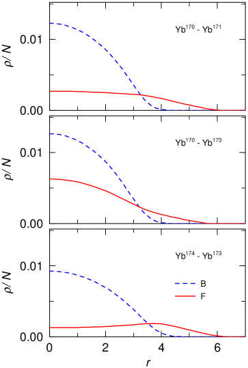
Figure 1: The ground-state density distributions of the BF mixtures: (a) ¹⁷⁰Yb$-^{171}$Yb, (b) ¹⁷⁰Yb$-^{173}$Yb and (c) ¹⁷⁴Yb$-^{173}$Yb (c). The dashed and solid lines represent the density of the bosons and fermions, respectively.

Thus obtained boson and fermion density distributions are shown in Figs. 1a-c. In the mixtures of ¹⁷⁰Yb$-^{171}$Yb  (Fig.1a) and ¹⁷⁰Yb$-^{173}$Yb  (Fig.1b), the density distributions are center-peaked, but, in the ¹⁷⁰Yb$-^{173}$Yb mixture, the fermion distribution has large overlap with the boson density, because of the attractive boson-fermion interaction ($h_{BF}<0$). On the other hand, in the ¹⁷⁴Yb$-^{173}$Yb mixture (Fig.1c), the fermion density distribution is surface-peaked; it is because the BF interaction is strong enough to satisfy the condition $h_{BF}/g_{BB}>1$ miyakawa . The $h_{BF}$-dependence of the fermion density distribution in the TF approximation is explained in Appendix A, where the ground-state density profiles are shown to be determined by the single parameter $h_{BF}/g_{BB}$.

III.2 Excitation Energies and Transition Strengths in RPA

As shown in the preceding calculations miyakawa ; tbDPL , the collective-oscillation frequency is sensitive to the profiles of the density distributions. Here we calculate the excited states in the random phase approximation (RPA), which is a good approximation in the case of the small amplitude, and show the transition strengths between the excited and ground states.

For this purpose, we calculate the fermion ground-state wave functions in the Hartree-Fock (HF) approximation and, then, the excited states are obtained using the ground state in RPA as in Ref. sogo .

In the HF approximation, the fermion number $N_{f}$ is restricted to the values that are determined from the subshell closure of fermion single-particle states, so that it become slightly different from the value of the present calculation; however, it does not affect the final results. The boson and fermion transition amplitudes from an excited state $|\Phi_{n}\rangle$ with the excitation energy $\omega_{n}$ to the ground state $|\Phi_{0}\rangle$ are defined by

$$T_{B}(\omega_{n}) = \langle\Phi_{n}|{\hat{O}}_{B}|\Phi_{0}\rangle,$$ (20)

$$T_{F}(\omega_{n}) = \langle\Phi_{n}|{\hat{O}}_{F}|\Phi_{0}\rangle,$$ (21)

where the quadrupole operators ${\hat{O}}_{B,F}$ are

$${\hat{O}}_{B} = \int d^{3}{r}\phi^{*}(\mbox{\boldmath$r$})(\mbox{\boldmath$r$}_{T}^{2}-2z^{2})\phi(\mbox{\boldmath$r$}),$$ (22)

$${\hat{O}}_{F} = \int d^{3}{r}\psi^{*}(\mbox{\boldmath$r$})(\mbox{\boldmath$r$}_{T}^{2}-2z^{2})\psi(\mbox{\boldmath$r$}).$$ (23)

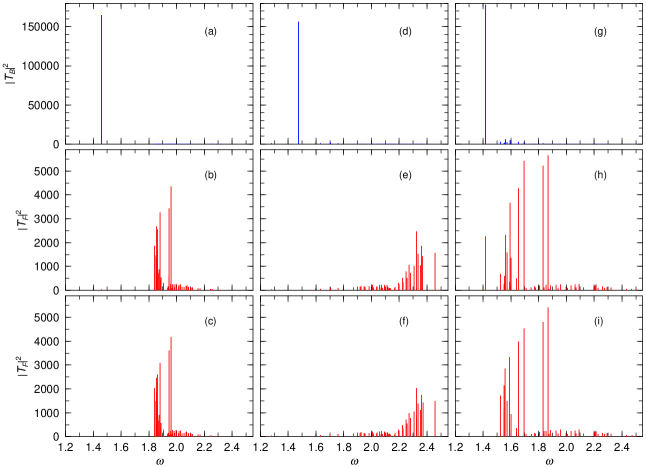
Figure 2: The transition strengths $|A_{B,F}|^{2}$ in RPA: ¹⁷⁰Yb$-^{171}$Yb (left panels), ¹⁷⁰Yb$-^{173}$Yb (center panels) and ¹⁷⁴Yb$-^{173}$Yb (right panels). The top, middle and bottom panels are for the boson, fermion and the single-particle fermion strengths

In Fig. 2, the transition strengths $|T_{B,F}|^{2}$ in RPA are shown for ¹⁷⁰Yb$-^{171}$Yb (left panels), ¹⁷⁰Yb$-^{173}$Yb (center panels) and ¹⁷⁴Yb$-^{173}$Yb (right panels) mixtures, where the boson and fermion transition strengths are plotted in the top and middle panels, respectively. In the bottom panels, the fermion strengths in the single particle processes are added.

As is clearly shown in the top panels, the boson transition strength $|T_{B}(\omega)|^{2}$ is almost concentrated on one excited state, whose excitation energy is denoted by $\omega_{Q}^{b}$. On the other hand, the fermion transition strength $|T_{F}(\omega)|^{2}$ have two peaks, and distribute between them (middle panels). In ¹⁷⁰Yb$-^{171}$Yb (left panels) and ¹⁷⁰Yb$-^{173}$Yb (center panels), the fermion strength $|T_{F}(\omega)|^{2}$ shows no sharp peaks at the boson excitation energy of $\omega_{Q}^{b}$; it has almost the same structure as the strength in the single particle process (bottom panels). In contrast, the ¹⁷⁴Yb$-^{173}$Yb mixture shows a visible strength at $\omega_{Q}^{b}$ (Fig. 2h), which is very small in the single particle process (Fig. 2i).

The two peaks of the fermion transition strength in the ¹⁷⁰Yb$-^{171}$Yb correspond to the fermion intrinsic modes. As shown in Ref. tbDPL , the fermion transition strength of the dipole oscillation also shows two peaks, which correspond to the fermion motions in the inside/outside regions of the bosons (the inside and outside fermion oscillations). Indeed, the second-peak frequency of the quadrupole oscillation is $\omega\approx 2$: the value in the pure harmonic oscillator potential. According to Ref. tbDPL , we call these two modes the mode-3 (the inside-fermion oscillation) and mode-2 (the outside-fermion oscillation), respectively; then, we define the fermion intrinsic frequency $\omega_{Q}^{f}$ as the peak position of the mode-3 in the fermion strength function $|T_{F}(\omega)|^{2}$. As shown in Fig. 2h, the $|T_{F}(\omega)|^{2}$ includes an additional mode. From Fig. 2g, we can find that it correspond to the oscillation forced by the boson intrinsic oscillation; we call it “the boson-forced oscillation” (mode-1).

It should be noted that, in the ¹⁷⁰Yb$-^{173}$Yb and ¹⁷⁴Yb$-^{173}$Yb mixtures, the fermion strength functions have two peaks (except the peak at $\omega=\omega_{Q}^{b}$) but no clear peaks at $\omega\approx 2$ corresponding to the mode-2 (Figs. 2e,h). It is because one of the two peaks (the stronger peak) are broad in these mixtures, and the two peaks are merged into one broad peak.

IV Quadrupole Oscillations of Boson-Fermion Mixtures of Yb Isotopes

In this section, we show the results of the time-evolution calculations for the quadrupole oscillations in the BF mixture.

IV.1 Time-Evolution of Boson-Fermion Mixtures and Description of Quadrupole Oscillations

As the initial condition of time-evolution at $\tau=0$, we take the boosted state from the ground-state condensed-boson wave function $\phi^{(g)}$ and fermion test particle momentum $(\mbox{\boldmath$p$}_{T}^{(g)},p_{z}^{(g)})$, which are defined by

$$\phi_{c}(\mbox{\boldmath$r$},\tau=0)=\exp\left\{\frac{i\lambda_{B}}{2\sqrt{2}}(r_{T}^{2}-2z^{2})\right\}\phi_{c}^{(g)}(\mbox{\boldmath$r$}),\noindent$$ (25)

and

$$\mbox{\boldmath$p$}_{T}(i)=\mbox{\boldmath$p$}_{T}^{(g)}(i)+m_{f}\omega_{f}\lambda_{F}\,\mbox{\boldmath$r$}_{T},\qquad p_{z}(i)=p_{z}^{(g)}(i)-2m_{f}\omega_{f}\lambda_{F}z.$$ (26)

In Eqs. (25) and (26), $\lambda_{B}$ and $\lambda_{F}$ are the boost parameters. Then, the boson and fermion current densities for the initial state become

$$\mbox{\boldmath$j$}_{B}(\mbox{\boldmath$r$},\tau=0) = \frac{\lambda_{B}}{\sqrt{2}}(\mbox{\boldmath$r$}_{T}-2z{\hat{z}})\rho_{B}^{(g)}(\mbox{\boldmath$r$}),$$ (27)

$$\mbox{\boldmath$j$}_{F}(\mbox{\boldmath$r$},\tau=0) = \omega_{f}\lambda_{F}(\mbox{\boldmath$r$}_{T}-2z{\hat{z}})\rho_{F}^{(g)}(\mbox{\boldmath$r$}).$$ (28)

In order to discuss the time-dependence of the quadrupole oscillations, we define the quantities $Q_{B,F}$ for boson and fermion:

$$Q_{B,F}=\frac{R_{T}^{2}(B,F)-2R_{L}^{2}(B,F)}{R_{0}^{2}(B,F)},$$ (29)

where

$$R_{T}^{2}(B,F) = \frac{1}{N_{b,f}}\int d^{3}{r}\,\mbox{\boldmath$r$}_{T}^{2}\rho_{B,F}(\mbox{\boldmath$r$}),$$ (30)

$$R_{L}^{2}(B,F) = \frac{1}{N_{b,f}}\int d^{3}{r}\,z^{2}\rho_{B,F}(\mbox{\boldmath$r$}),$$ (31)

and $R_{0}(B)$ and $R_{0}(F)$ are the root-mean-square radii of the boson and fermion distributions in the ground state.

In the case of no BF interactions ($h_{BF}=0$), the quantities $Q_{B}$ and $Q_{F}$ are proportional to $\lambda_{B}\sin(\sqrt{2}\tau)$ and $\lambda_{F}\sin(2\omega_{f}\tau)$, respectively; they oscillate monotonously with the periods $\sqrt{2}$ and $2\omega_{f}$.

When the amplitude is not small, the oscillations are also not simple and include various modes. In order to separate these modes, we use the strength functions $S_{B,F}(\omega)$, which is defined as the Fourier transform of $Q_{B,F}$:

$$S_{B,F}(\omega)=\int^{t_{f}}_{t_{i}}d\tau\,Q_{B,F}(\tau)\sin{\omega\tau}$$ (32)

where we use the oddness $Q_{B,F}(\tau)=-Q_{B,F}(-\tau)$. It is expected from the initial conditions in Eqs. (25) and (26) because they lead to $Q_{B,F}=0$ and $dQ_{B,F}/d\tau\neq 0$ at $\tau=0$. For the time-integration in Eq. (32), we use the interval $0<\tau<200$ unless otherwise noted.

Finally, we mention how the time-dependence of the collective oscillations obtained in the time-evolution method should be compared with the strength function in RPA in comparison. The initial boosted state corresponding to the initial condition in Eqs. (25) and (26) is given by

$$|\Phi(\tau=0)\rangle=e^{\frac{i}{2}\left\{\kappa_{B}{\hat{O}}_{B}+\kappa_{F}{\hat{O}}_{F}\right\}}|\Phi_{0}\rangle,$$ (33)

where $|\Phi_{0}\rangle$ is the ground state, ${\hat{O}}_{B,F}$ are the quadrupole operators defined in Eqs. (22) and (23), and $\kappa_{B,F}$ correspond to the boost parameters. Expanding $|\Phi(\tau=0)\rangle$ with respect to $\kappa_{B,F}$, Eq. (33) becomes

$$|\Phi(\tau=0)\rangle \approx |\Phi_{0}\rangle+\frac{i}{2}\left\{\kappa_{B}{\hat{O}}_{B}+\kappa_{F}{\hat{O}}_{F}\right\}|\Phi_{0}\rangle$$ (34)

$$= |\Phi_{0}\rangle+\frac{i}{2}\sum_{n}\left\{\kappa_{B}T_{B}(\omega_{n})+\kappa_{F}T_{F}(\omega_{n})\right\}|\Phi_{n}\rangle,$$

where the transition amplitudes $T_{B,F}(\omega_{n})$ are given in Eqs. (20) and (21). Thus, using the strength functions $T_{B,F}$, which is obtained in RPA, the time-dependent functions $Q_{B,F}$ are represented by

$$Q_{B}(\tau) = \frac{1}{N_{b}R_{0}^{2}(B)}\sum_{n}T_{B}(\omega_{n})\left\{\kappa_{B}T_{B}(\omega_{n})+\kappa_{F}T_{F}(\omega_{n})\right\}\sin(\omega_{n}\tau),$$ (35)

$$Q_{F}(\tau) = \frac{1}{N_{f}R_{0}^{2}(F)}\sum_{n}T_{F}(\omega_{n})\left\{\kappa_{B}T_{B}(\omega_{n})+\kappa_{F}T_{F}(\omega_{n})\right\}\sin(\omega_{n}\tau).$$ (36)

Also, in RPA, the strength functions become

$$S_{B}(\omega) = \frac{1}{2N_{b}}\sum_{n}T_{B}(\omega_{n})\left\{\kappa_{B}T_{B}(\omega_{n})+\kappa_{F}T_{F}(\omega_{n})\right\}F_{n}(t_{f},t_{i}),$$ (37)

$$S_{F}(\tau) = \frac{1}{2N_{f}}\sum_{n}T_{F}(\omega_{n})\left\{\kappa_{B}T_{B}(\omega_{n})+\kappa_{F}T_{F}(\omega_{n})\right\}F_{n}(t_{f},t_{i}),$$ (38)

where

$$F_{n}(t_{f},t_{i})=\frac{\sin{(\omega-\omega_{n})t_{f}}-\sin{(\omega-\omega_{n})t_{i}}}{2(\omega-\omega_{n})}-\frac{\sin{(\omega+\omega_{n})t_{f}}-\sin{(\omega+\omega_{n})t_{i}}}{2(\omega+\omega_{n})}.$$ (39)

In the case of extremely small amplitude, the TDGP+Vlasov (time-evolution) approach and RPA should give the same results for the corresponding boost parameters: $\kappa_{B}=\lambda/\sqrt{2}$ and $\kappa_{F}=\lambda_{F}$; it has been really confirmed in the case of dipole oscillations tbDPL . However, in the present calculation where the amplitude is not so small, the TDHF and Vlasov approach does not give the same results with those in RPA; especially, in the later stage of time-evolution. Thus, we use the corresponding values of $\kappa_{B(F)}$ in RPA as to reproduce the oscillations in early stage of time-evolution in the TDGP and Vlasov approach.

IV.2 Quadrupole Oscillations in ¹⁷⁰Yb$-^{171}$Yb

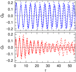
Figure 3: Time evolution of the quadrupole oscillations in the ¹⁷⁰Yb$-^{171}$Yb mixture with the in-phase initial condition $\lambda_{B}=\lambda_{F}=0.1$. The upper and lower panels are $Q_{B,F}$ for the bosons and fermions, and the solid and dashed lines represent the results of TDGP + Vlasov and RPA calculations.

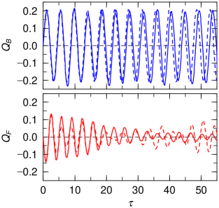
Figure 4: Time evolution of the quadrupole oscillations in the ¹⁷⁰Yb$-^{171}$Yb mixture with the out-of-phase initial condition $\lambda_{B}=-\lambda_{F}=0.1$. The panels and the lines are the same as in Fig. 3.

First, we discuss the quadrupole oscillation in ¹⁷⁰Yb$-^{171}$Yb system, where the boson-fermion interaction is weekly repulsive. In Fig. 3, we show the time-dependences of the $Q_{B}$ (the upper panel) and $Q_{F}$ (the lower panel) for the initial condition $\lambda_{B}=\lambda_{F}=0.1$, which corresponds to the “in-phase” boson-fermion oscillation. The dashed and solid lines represent the results of the TDGP+Vlasov and RPA calculations, respectively. Furthermore, we also show the results for the initial condition of the “out-of-phase” boson-fermion oscillation: $\lambda_{B}=-\lambda_{F}=0.1$ in Fig. 4.

In both cases, the results of the TDGP+Vlasov calculation agree well with those in RPA in the early stage of time-evolution ($\tau\lesssim 20$). In RPA, the fermion oscillations show clear beating; the amplitudes gradually decrease around $\tau\approx 35$ and become larger after that. In the TDGP+Vlasov approach, the amplitudes are also damped but does not show clear beat phenomena.

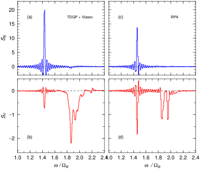
Figure 6: The strength functions of the quadrupole oscillations with the out-of-phase initial condition in ¹⁷⁰Yb$-^{171}$Yb  mixture (corresponding to Fig. 4); The panels and the lines are the same with Fig. 5.

Next we calculate the strength functions $S_{B,F}$ for these oscillations using Eqs. (32) with integrating over the range of $0\leq\tau\leq 200$. Figs. 5 and 6 show the $S_{B,F}$ for the oscillations with the in-phase and out-of-phase initial conditions; the boson and fermion strength functions in TDGP+Vlasov calculation are in the upper left (a) and the lower left (b) panels, and those in RPA are in the upper right (c) and the lower right (d) panels.

In these figures, we find that the boson strength functions $S_{B}$ have only one sharp peak, which is consistent with the monotonous behavior of $Q_{B}(\tau)$ in Figs. 3 and 4. In contrast, the fermion strength functions $S_{F}$ has one negative peak at $\omega=\omega_{Q}^{b}$ and two peaks at $\omega\approx 1,87$ and $\approx 1.96$; these two peaks are positive in the in-phase initial condition and negative in the out-of-phase initial condition.

These behaviors are very similar to those in the dipole oscillations tbDPL . The peaks at $\omega\approx\omega_{Q}^{b}$ and at $\omega\approx 1.87$ correspond to the boson-forced oscillation (mode-1). and the inside-fermion oscillation (mode-3), respectively. In addition, we see a small peak at $\omega\approx 1.96$, which correspond to the outside-fermion oscillation (mode-2). In TDGP+ Vlasov calculations, these peaks have broader widths than in RPA, so that the strengths of the outside-fermion oscillation (mode-2) in TDGP+Vlasov calculation are not so clear (Figs. 3b and 4b).

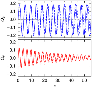
Figure 7: Time evolution of the quadrupole oscillations with the in-phase initial condition in the BF mixture with $h_{BF}=-1.9680$; other parameters are the same as in ¹⁷⁰Yb$-^{171}$Yb case. The panels and the lines are the same as in Fig. 5.

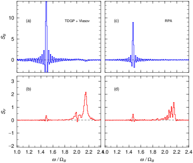
Figure 8: The strength functions of the quadrupole oscillations corresponding to Fig. 7; other parameters are the same as in ¹⁷⁰Yb$-^{171}$Yb case. The panels and the lines are the same as in Fig. 5.

In order to examine the sign-dependence of the boson-fermion coupling constant $h_{BF}$, we perform an additional simulation with the attractive boson-fermion coupling constant with $h_{BF}=-1.9680$ (and the same values for the other parameters as in ¹⁷⁰Yb$-^{171}$Yb ). In Figs. 7 and 8, we show the time-evolutions $Q_{B,F}$and the strength functions $S_{B,F}$ with the in-phase initial condition. The TDGP+Vlasov and RPA calculations give almost the same results. In this case, the fermion oscillation shows no beats in both approaches (Fig. 7, bottom). In the strength functions (Fig. 8), the peak of the fermion oscillation at $\omega=\omega_{Q}^{b}$ becomes positive, and its heights becomes smaller than that in Fig. 5. We also see a peak at $\omega\approx 1.99$ in $S_{F}$ in the TDGP+Vlasov calculation (Fig. 8b), which corresponds to the outside-fermion oscillation (mode-2), but no clear peaks are found around this frequency in the RPA calculation. In the case of attractive boson-fermion interaction, more fermions populate in the boson-distributed region, and it makes the outside-fermion oscillation (mode-2) strength small. Thus, the strength of the mode-2 becomes very small in the small-amplitude oscillations described in RPA. As the amplitude becomes larger, however, more fermions move to the outside from the boson-distributed region, and the strength of the mode-2 becomes larger in TDGP+Vlasov approach.

IV.3 Quadrupole Oscillations in ¹⁷⁰Yb$-^{173}$Yb

In this subsection, we discuss the quadrupole oscillations in the ¹⁷⁰Yb$-^{173}$Yb system, where the boson-fermion interaction is strongly attractive.

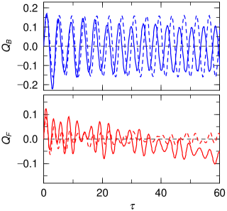
Figure 9: Time evolution of the quadrupole oscillations in the ¹⁷⁰Yb$-^{173}$Yb mixture with the in-phase initial condition $\lambda_{B}=\lambda_{F}=0.1$. The upper and lower panels are $Q_{B,F}$ for the bosons and fermions, and the solid and dashed lines represent the results of TDGP + Vlasov and RPA calculations.

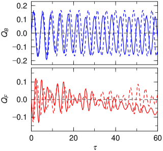
Figure 10: Time evolution of the quadrupole oscillations in the ¹⁷⁰Yb$-^{173}$Yb mixture with the out-of-phase initial condition $\lambda_{B}=-\lambda_{F}=0.1$. The panels and the lines are the same as in Fig. 9.

In Figs. 9 and 10, we show the time-dependence of the $Q_{B,F}$ in ¹⁷⁰Yb$-^{173}$Yb system for two kinds of initial conditions, $\lambda_{B}=\lambda_{F}=0.1$ (in-phase) and $\lambda_{B}=-\lambda_{F}=0.1$ (out-of-phase), respectively.

Figs. 9 and 10 clearly show that the TDGP+Vlasov calculation gives very different results from RPA in this BF mixture. The boson oscillations in the TDGP+Vlasov calculation have slight damping, and shorter periods than those in RPA. Furthermore, $Q_{F}$ decrease in the TDGP+Vlasov calculation and become negative when $\tau\gtrsim 40$ (bottom panels). In comparison with RPA, the TDGP+Vlasov calculation shows slightly shorter periods in the bose oscillations and exhibit slight dampings (top panels).

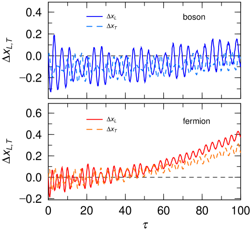
Figure 11: Time evolution of $R_{z}$ (solid lines) and $R_{T}$ (dotted lines) for the quadrupole oscillation in ¹⁷⁰Yb$-^{173}$Yb mixture with the in-phase initial condition (corresponding to Fig. 9); the upper and lower panels are for the bosons and fermions.

In order to examine these results further, we calculate the deformation shifts in the longitudinal and transversal directions: $\Delta x_{L}=\sqrt{3}R_{L}/R_{0}-1$ and $\Delta x_{T}=\sqrt{3/2}R_{T}/R_{0}-1$, where $R_{0,L,T}$ are the root-mean-square radii of the ground and the oscillation states, which are defined in Eqs. (30) and (31). The time-dependences of $\Delta x_{L,T}$ are plotted in Fig. 11 in the case of the in-phase initial condition. In these figures, we can find the increase of the fermion radii in both directions; namely the expansion of the fermion gas occurs in the oscillation process. We can also find $R_{L}>R_{T}$ for the fermion oscillations in this expanding process; from the definition of $Q_{F}$ in (29), it is just the origin of $Q_{F}<0$ (Figs. 9 and 10, bottom). This expansion can be understood by the fermion overflow from the boson-distributed region; in the ground state, fermions populate largely in the boson-distributed region because of the attractive BF interaction, but, in the excited sate, some of them are pushed into the outside in the course of oscillation. Such expansion has already been discussed theoretically in the monopole oscillation monoEX .

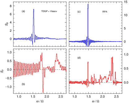
Figure 12: The strength functions of the quadrupole oscillations with the in-phase initial condition in ¹⁷⁰Yb$-^{173}$Yb  mixture (corresponding to Fig. 9); the panels and lines are the same as in Fig. 5.

The strength functions $S_{B,F}$ corresponding to these oscillations are shown in Figs. 12 (in-phase) and 13 (out-of-phase), respectively. In RPA calculations (Figs. 12c,d and 13c,d), the $S_{B,F}$ have a clear peak at $\omega\approx 1.4$ and a broad peak around $\omega\approx 2.3$, which correspond to the boson-forced (mode-1) and the inside-fermion (mode-3) oscillations. No peaks exist, which correspond to the outside oscillation (mode-2). It is because, in the ground state, the attractive interaction makes a large part of fermions populate in the boson-distributed region so that the fermions that exist outside region gives very small contribution in $S_{B,F}$.

The TDGP+Vlasov calculation gives similar results for the $S_{B}$ with those in RPA (Figs. 12a and 13a); however, the $S_{F}$ are quite different (Figs. 12b and 13b). In the TDGP+Vlasov calculation, the $S_{F}$ have no clear peak at $\omega\approx 1.4$, which corresponds to the boson-forced oscillation (mode-1), but have a broad peak appears around $\omega\approx 2.3$. Also the strength below $\omega\lesssim 1.4$ monotonously increases as $\omega$ becomes smaller; these monotonous behaviors in the $S_{F}$ are also caused by the expansion of the fermion gases.

Furthermore, we see an unclear peak around $\omega\approx 1.85$ in the $S_{F}$ (Fig. 12d). As mentioned before, the $Q_{F}$ is assumed to be an odd function for the time parameter $\tau$, but the calculated strength function does not seem to be the odd function around this peak. In order to clarify the situation, we calculate the absolute strength function:

$$A_{B,F}(\omega)=\left|\int^{t_{f}}_{t_{i}}d\tau Q_{B,F}(\tau)e^{i\omega\tau}\right|.$$ (40)

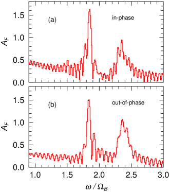
Figure 14: The fermion absolute strength functions of the quadrupole oscillations in ¹⁷⁰Yb$-^{173}$Yb gas with the in-phase and the out-of-phase initial conditions.

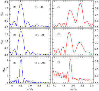
Figure 15: The absolute strength functions of the quadrupole oscillations in ¹⁷⁰Yb$-^{173}$Yb mixtures with the in-phase initial conditions; the left (B1,B2,B3) and right (F1,F2,F3) panels are for the boson and fermion oscillations. The strength functions are deduced from the evolution in $0<\tau<25$ (the top panels), in $25<\tau<50$ (the middle panels) and in $50<\tau<100$ (the bottom panels), respectively.

The results are shown in Fig. 14a,b for the oscillations with the in-phase and the out-of-phase initial conditions. Two clear peaks are seen at $\omega=1.85$ and 2.35 in both cases. To make clear the origin of these peaks, we divide the oscillation period into three regions $0<\tau<25$ (F1, early stage), $25<\tau<50$ (F2, intermediate stage) and $50<\tau<100$ (F3, later stage), and evaluate the $A_{F}(\omega)$ in these stages. As shown in Fig. 15, the peak of the $S_{F}$ appears around $\omega=2.35$ in the early stage (panel F1), but disappear in the latter stage (panel F3). In contrast, the peak at $\omega=1.85$ is seen in all stages.

Because of the large expansion of the fermion gas, which is shown in Fig. 11, the quadrupole oscillations are supposed to couple with the monopole oscillation mode. For examination, we calculate the strength function of the monopole oscillation mode:

$$A^{M}_{B,F}(\omega)=\left|\int^{t_{f}}_{t_{i}}d\tau\left[\frac{R(B,F)}{R_{0}(B,F)}-1\right]e^{i\omega\tau}\right|,$$ (41)

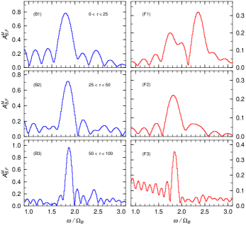
Figure 16: The absolute strength functions of the monopole oscillations in ¹⁷⁰Yb$-^{173}$Yb mixtures with the in-phase initial conditions. The panels are the same as in Fig. 15.

which are plotted in Fig. 16 for the three stages: $0<\tau<25$ (B1,F1), $25<\tau<50$ (B2,F2) and $50<\tau<100$ (B3,F3). The fermion strength function has a peak at $\omega\approx 2.35$ in early stage (F1) but it disappear in later stage (F2,F3); on the other hand, the peak at $\omega\approx 1.85$ can be seen in all stages. Thus, we can find that the peak at $\omega\approx 1.85$ in the $S_{F}$ of the quadrupole oscillation corresponds to the monopole mode, which is excited through the expansion of the fermion gas; it explains the asymmetry of the $S_{F}$ around the peak.

From the above analysis, we can obtain the following picture on the quadrupole oscillation in the ¹⁷⁰Yb$-^{173}$Yb mixture: 1) The strongly-attractive boson-fermion interaction makes a large part of fermions populate in the boson-distributed region in the ground state. 2) In the quadrupole oscillation, the oscillating bosons causes the fermion overflow from this region and it caused the expansion of the fermion gas. 3) The initial conditions in the present calculation breaks the rotation symmetry, and, in the large-amplitude oscillation, the angular momentum becomes much larger than $2\hbar$. It can excite the monopole mode through the oscillation. As a result, the oscillations include both the monopole and quadrupole modes. 4) In the course of the fermion gas expansion, the intrinsic modes of the fermion quadrupole oscillation (mode-2 and -3) are damped and loses its strength in early stage; instead, the monopole oscillation mode grows up. 5) In addition the expansion process of the fermion gas is slow and not collective, and then many small modes appear below $\omega\lesssim 1.5$.

IV.4 Quadrupole Oscillations in ¹⁷⁴Yb$-^{173}$Yb

Finally, we discuss the quadrupole oscillations in the ¹⁷⁴Yb$-^{173}$Yb mixture, where the boson-fermion interaction is strongly repulsive and, different from other two mixtures, the fermion density distribution is surface-peaked.

When $h_{BF}>g_{BB}$, the effective potential for fermions has the minimum in the surface of the boson-distributed region, which produce the surface-peaked fermion-density distributions in the ground state; in the oscillation mode, the fermion gas is considered to oscillate in the neighborhood of this minimum.

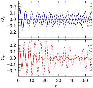
Figure 17: Time evolution of the quadrupole oscillations in the ¹⁷⁴Yb$-^{173}$Yb mixture with the in-phase initial condition $\lambda_{B}=\lambda_{F}=0.1$. The upper and lower panels are $Q_{B,F}$ for the bosons and fermions, and the solid and dashed lines represent the results of TDGP + Vlasov and RPA calculations.

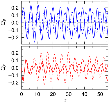
Figure 18: Time evolution of the quadrupole oscillations in the ¹⁷⁴Yb$-^{173}$Yb mixture with the out-of-phase initial condition $\lambda_{B}=-\lambda_{F}=0.1$. The panels and the lines are the same as in Fig. 9.

Figs. 17 and 18 show the time-dependence of the $Q_{B,F}$ for the in-phase and out-of-phase initial conditions; the dashed and solid lines are for the TDGP+Vlasov and RPA calculations. These two calculations are consistent within one cycle of oscillation, but become very different after that. In the TDGP+Vlasov calculations, the amplitude of the fermion oscillation shows quick damping, and the boson oscillations exhibits beating and small damping in the case of the in-phase initial condition (Fig. 18).

The similar damping phenomena have already been appeared in the monopole tomoBF and dipole oscillations tbDPL ; however, in these oscillations, the boson oscillations are stable and simply affects the fermion motions through the strong repulsive BF interactions, for quick dampings of the fermion oscillations decrease the strength of their intrinsic mode soon.

In Fig. 19, we show those oscillations in later stage $60<\tau<120$ in the cases of the in-phase (a) and the out-of-phase (b) initial conditions. We see that the oscillations keep the almost constant amplitudes in this stage, and the bosons and fermions oscillate in out-of-phase with the same periods of oscillations. These results shows that the intrinsic fermion mode loses the strength in early stage, and only the forced-oscillation mode survives for a long time.

This mixture prefers the BF out-of-phase oscillation; even if the oscillation starts with the in-phase oscillation, the relative phase shift occurs and the oscillation becomes the out-of-phase. At the time of the phase change, the oscillation accompanies large diffusion. Thus, the $Q_{F}$ shows strong damping, and the $Q_{B}$ also shows small damping and beating throughout the process.

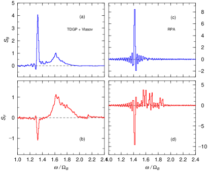
Figure 20: The strength functions of the quadrupole oscillations with the in-phase initial condition in ¹⁷⁴Yb$-^{173}$Yb mixture (corresponding to Fig. 17); the panels and lines are the same as in Fig. 5.

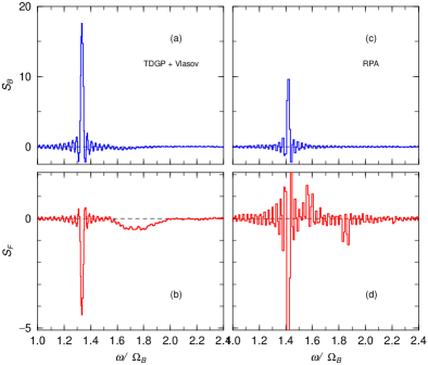
Figure 21: The strength functions of the quadrupole oscillations with the out-of-phase initial condition in ¹⁷⁰Yb$-^{173}$Yb  mixture (corresponding to Fig. 18); The panels and the lines are the same with Fig. 5.

Next, we show the strength functions $S_{B,F}$ in Fig. 20 (in-phase initial condition) and in Fig. 21 (out-of-phase initial condition). In RPA, the boson strengths concentrate on one sharp peak (Fig. 20c and Fig. 21c), and the fermion strengths have one sharp peak at the same frequency with the $S_{B}$ and have small peaks with broad widths (Fig. 20d and Fig. 21d); in these results, the $S_{F}$ show no strong intrinsic oscillation modes.

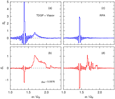
Figure 22: The strength functions of the quadrupole oscillations with the in-phase initial condition in BF mixture with $g_{BB}=5.5976$ (other parameters are the same as ¹⁷⁰Yb$-^{173}$Yb  mixture); the panels and lines are the same as in Fig. 5.

Here we should note that the boson-boson scattering lengths are very different in ¹⁷⁴Yb and ¹⁷⁰Yb as shown in TABLE I; thus, the boson-boson coupling constant $g_{BB}$ in ¹⁷⁴Yb$-^{173}$Yb mixture becomes different from that in the other mixtures. As shown in Appendix A, in the TF approximation, the ground state depends only on the ratio $h_{BF}/g_{BB}$, and not on $g_{BB}$ directly. In order to show this coupling-constant dependence, we calculate the quadrupole oscillation of the mixture with $g_{BB}=5.598\times 10^{-2}$ and $h_{BF}=7.420\times 10^{-2}$, which is chosen to have the same value of the coupling-constant ratio with the ¹⁷⁴Yb$-^{173}$Yb mixture $h_{BF}/g_{BB}=1.325$. The strength functions of the quadrupole oscillations are shown in Fig. 22, which should be compared with Fig. 20 for the ¹⁷⁴Yb$-^{173}$Yb mixture. We find that hight of several peaks are different, but their positions are the same in these figures. It confirms that the frequencies of the oscillation modes are determined by the ratio $h_{BF}/g_{BB}$ only though peak heights depend on two parameters $g_{BB}$ and $h_{BF}$.

IV.5 Fermion Intrinsic Modes and Comparison with Sum-rule Approach

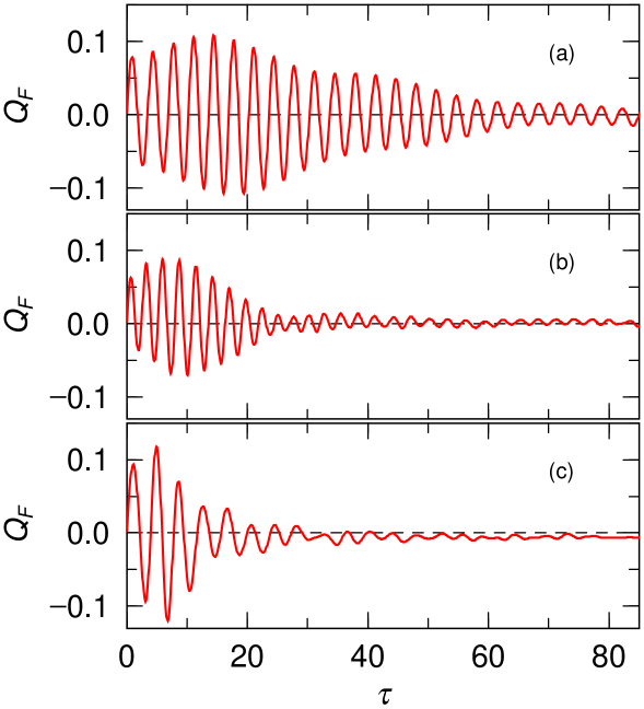
Figure 23: Time evolution of the quadrupole fermion oscillations in ¹⁷⁰Yb$-^{171}$Yb (a), ¹⁷⁰Yb$-^{171}$Yb (b) and ¹⁷⁰Yb$-^{171}$Yb (c), where the boson motions are frozen. The initial condition is given by $\lambda_{F}=0.1$ for all cases.

In order to have some additional discussion about the fermion intrinsic modes, we calculate the fermion oscillation when the boson motion is frozen. In Fig. 23, we show the results for the mixtures of ¹⁷⁰Yb$-^{171}$Yb (a), ¹⁷⁰Yb$-^{173}$Yb (b) and ¹⁷⁴Yb$-^{173}$Yb (c); the dampings in ¹⁷⁰Yb$-^{173}$Yb and ¹⁷⁴Yb$-^{173}$Yb are found to be much faster than that in ¹⁷⁰Yb$-^{171}$Yb .

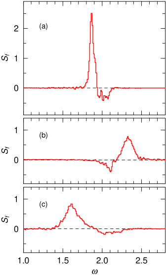
Figure 24: The fermion strength functions of the fermion quadrupole oscillations corresponding to the cases in Fig. 23.

The fermion strength functions $S_{F}$ of these mixtures are shown in Fig. 24. It is found that the $S_{F}$ show a large positive and a small negative peaks. The positions of the positive peak, which are different in these three mixtures, are at the inside-fermion oscillation frequencies (mode-3) obtained in the previous calculations. The small peaks are located in $2.0\leq\omega\leq 2.1$; they are supposed to be the outside-fermion oscillations (mode-2) in the previous calculations.

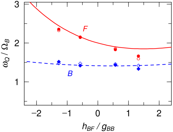
Figure 25: Intrinsic frequencies of the quadrupole oscillations in boson (diamonds) and fermion (circles) components of the BF mixtures in the TDGP+Vlasov (full diamonds and circles) and RPA (open diamonds and circles) calculations. The solid and dashed lines are for the sum-rule results of the boson and fermion quadrupole modes.

These peaks have broad widths, and it suggests that the oscillation modes corresponding to them have large dampings. Particularly, the outside-fermion mode has very low peak, so that it does not play any significant roles in the full calculations in the previous section. As the absolute value of the boson-fermion coupling increases, the effective potential for fermions has large deformation from the harmonic oscillator shape, and the unharmonic effect from this deformation makes large dampings of the fermion intrinsic modes, and the boson-forced oscillation mode (mode-1) have larger contribution in the full calculation. We show the $h_{BF}$-dependence of the boson and fermion intrinsic frequencies in Fig. 25, which are defined as peak positions of the strength functions.

Now we should give some comments on the results by the sum-rule approach miyakawa In the sum-rule approach, the intrinsic frequencies of the boson and fermion quadrupole oscillations are obtained by

$$\omega_{Q}^{b} = \sqrt{2-\frac{1}{N_{b}R_{B}^{2}}V_{QP}},$$ (42)

$$\omega_{Q}^{f} = \sqrt{\frac{1}{R_{B}^{2}}K_{F}+2\omega_{f}^{2}-\frac{1}{m_{f}N_{f}R_{F}^{2}}V_{QP}},$$ (43)

where

$$K_{F} = \frac{1}{10\pi^{2}m_{f}^{2}}\int d^{3}{r}(6\pi\rho_{F})^{\frac{5}{3}},$$ (44)

$$V_{QP} = -\frac{8}{5}h_{BF}\int d^{3}{r}r^{2}\frac{\partial\rho_{B}}{\partial r}\frac{\partial\rho_{F}}{\partial r}.$$ (45)

The solid and dashed lines Fig. 25 show the frequencies of the fermion and boson quadrupole oscillation obtained in the sum-rule approach.

The results of the sum-rule approach well reproduce the TDGP+Vlasov and RPA calculations, except the fermion intrinsic frequencies at $h_{BF}/g_{BB}=1.3256$. It should be noted that, when $h_{BF}/g_{BB}>1$, the fermion density becomes surface-peaked, and $V_{QP}<0$, so that, in the sum-rule approach, the intrinsic frequencies take minimum values at $h_{BF}/g_{BB}\approx 1$ as shown in Fig. 25, and increase $h_{BF}/g_{BB}>1$.

As mentioned before, when $h_{BF}/g_{BB}>1$, the density- and velocity-distribution changes occur through the oscillation in the case of the large amplitudes, and the potential minimum for the fermion, which exists at the border of the boson-distributed region, also changes its position. Thus, it causes the smaller intrinsic frequency of fermion ($\omega_{Q}^{f}$) than the result obtained in the sum-rule approach, because the sum-rule approach assumes the small amplitude oscillations, and the density-distribution changes through oscillation are not included.

Anyway, in the case of the repulsively-strong boson-fermion interaction, the peak of the fermion strength function is small and broad, and the contribution from the fermion intrinsic mode is not so large except early stage in oscillation.

V Summary

In this paper, we have investigated the collective quadrupole oscillation in three kinds of the BF mixtures of the Yb isotopes: ¹⁷⁰Yb$-^{171}$Yb , ¹⁷⁰Yb$-^{173}$Yb and ¹⁷⁴Yb$-^{173}$Yb , where the boson-fermion interactions are weakly repulsive, strongly attractive and strongly repulsive. In actual numerical calculations, we have obtained the time-evolutions of the oscillating mixtures directly using the TDGP and Vlasov equations, and compare the results with the RPA calculations.

Theoretically, these two approaches predict the same modes of oscillations: the intrinsic (mode-2,3) and boson-forced (mode-1) oscillations. Nevertheless, the oscillation behaviors are quite different in these two approaches, especially in later stage of oscillation.

When the boson-fermion interaction is weak, the two approaches give almost the same results in early stage, but some difference appears in latter stage. In the mixture with very strong BF interaction, the difference appears also in the earlier stage; in ¹⁷⁰Yb$-^{173}$Yb and ¹⁷⁴Yb$-^{173}$Yb mixtures, the two approaches are consistent only in the first one or two periods of the oscillations.

In the case of the strongly-attractive BF interaction (¹⁷⁰Yb$-^{173}$Yb ), the fermion overflow from the boson-distributed region into the outside causes the fermion gas expansion. On the other hand, When the BF interaction is strongly repulsive (¹⁷⁴Yb$-^{173}$Yb ), the fermion oscillation loses the strength of its intrinsic mode soon, and the fermi gas oscillates with the same period of the boson gas in later period.

The RPA is available only in the case of the small-amplitude oscillations, because it cannot trace the density-distribution changes in the course of time evolution. In actual experiments, the amplitude is not so small, and the methods in solving the time-dependence process should be proper in comparison with experiments.

In this paper, we assume the spherical trapping potential with $\kappa_{L}=1$, but the actual experiments will be done with the largely-deformed potential with $\kappa_{L}=1/6$, for example, in Kyoto group. In such cases, the breathing oscillations are not decoupled into the monopole and quadrupole modes scalTF2 but into the longitudinal and transverse oscillation modes. The results of the collective oscillations of the BF mixtures in the deformed trapping potential will be discussed in another paper MYnext .

Furthermore, we do not take into account two-body collisions and thermal boson effects JackZar . In the system $N_{b}\gg N_{f}$ at $T=0$, the number of thermal bosons are very small, so that the two-body collisions are not expected to play any significant roles in the oscillation processes. In the actual experiments, which are performed at very low but $T\neq 0$ temperatures, thermal bosons should give some contributions; the introduction of such effects through two-body collision terms into our approach should be done in the future BUU1 ; TOMO1 .

Appendix A Ground State of Boson-Fermion Mixtures in Thomas-Fermi Approximation

In this appendix, we briefly explain the ground state of the BF mixture in the Thomas-Fermi (TF) approximation.

In this approximation, the total energy of the BF mixture is given by

$$E_{T}=\int d^{3}{r}\Bigg{\{} \frac{1}{2}(\mbox{\boldmath$r$}_{T}^{2}+\kappa_{L}^{2}r_{3}^{2})\rho_{B}(\mbox{\boldmath$r$})+\frac{g_{BB}}{2}\rho_{B}^{2}(\mbox{\boldmath$r$})$$ (46)

$$+ \frac{1}{20\pi^{2}m_{f}}[6\pi\rho_{F}(\mbox{\boldmath$r$})]^{5/3}+\frac{1}{2}m_{f}\omega_{f}^{2}(\mbox{\boldmath$r$}_{T}^{2}+\kappa_{L}^{2}r_{3}^{2})\rho_{F}(\mbox{\boldmath$r$})$$

$$+ h_{BF}\rho_{B}(\mbox{\boldmath$r$})\rho_{F}(\mbox{\boldmath$r$})\Bigg{\}},$$

The scaled dimensionless variables and parameters are defined by

$$h=\frac{1}{m_{f}\omega_{f}^{2}}\frac{h_{BF}}{g_{BB}}, \mbox{\boldmath$x$}=\frac{m_{f}^{4}\omega_{f}^{5}g_{BB}}{3\pi^{2}}(r_{1},r_{2},\kappa_{L}r_{3}),$$

$$n_{B}=\frac{2m_{f}^{8}\omega_{f}^{10}g_{BB}^{3}}{9\pi^{4}}\rho_{B}, n_{F}=\frac{2m_{f}^{9}\omega_{f}^{12}g_{BB}^{3}}{9\pi^{4}}\rho_{F},$$

$$e_{B}=\frac{2m_{f}^{8}\omega_{f}^{10}g_{BB}^{2}}{9\pi^{4}}\mu_{B}, e_{F}=\frac{2m_{f}^{7}\omega_{f}^{8}g_{BB}^{2}}{9\pi^{4}}\mu_{F}.$$ (47)

The effective boson and fermion numbers are defined by

$${\tilde{N}}_{B} = \int d^{3}xn_{B}=\frac{2\kappa_{L}m_{f}^{20}\omega_{f}^{25}g_{BB}^{6}}{3^{5}\pi^{10}}N_{B},$$ (48)

$${\tilde{N}}_{F} = \int d^{3}xn_{F}=\frac{2\kappa_{L}m_{f}^{21}\omega_{f}^{27}g_{BB}^{6}}{3^{5}\pi^{10}}N_{F}.$$ (49)

Finally, the scaled total energy becomes

$${\tilde{E}}_{T} = \frac{2\kappa_{L}m_{f}^{28}\omega_{f}^{35}g_{BB}^{8}}{3^{7}\pi^{14}}E_{T}$$ (50)

$$= \int d^{3}{x}\left\{x^{2}n_{B}+\frac{1}{2}n_{B}^{2}+\frac{3}{5}n_{F}^{\frac{5}{3}}+x^{2}n_{F}+hn_{B}n_{F}\right\},$$

where $x^{2}=|\mbox{\boldmath$x$}|^{2}$.

Let’s introduce the particle-number constraints into the total energy as ${\tilde{E}}^{\prime}=\mbox{${\tilde{E}}_{T}$}-e_{B}\mbox{${\tilde{N}}_{B}$}-e_{F}\mbox{${\tilde{N}}_{F}$}$, where the Lagrange multipliers $e_{B}$ and $e_{F}$ are the scaled boson and fermion chemical potentials. The variations of ${\tilde{E}}^{\prime}$, $\delta{\tilde{E}}^{\prime}/\delta n_{B}=0$ and $\delta{\tilde{E}}^{\prime}/\delta n_{F}=0$, gives the TF equations for the ground-state densities $n_{B,F}$

$$n_{B}+hn_{F} = e_{B}-x^{2},$$ (51)

$$n_{F}^{\frac{2}{3}}+hn_{B} = e_{F}-x^{2},$$ (52)

The second order variations give the stability condition of the TF ground states:

$$\frac{\delta^{2}\mbox{${\tilde{E}}_{T}$}}{\delta n_{B}^{2}}\frac{\delta^{2}\mbox{${\tilde{E}}_{T}$}}{\delta n_{F}^{2}}-\left(\frac{\delta^{2}\mbox{${\tilde{E}}_{T}$}}{\delta n_{B}\delta n_{F}}\right)^{2}>0,$$ (53)

which leads to

$$n_{F}^{1/3}<\frac{2}{3h^{2}}.$$ (54)

It should be noted that the scaled equations include three parameters, $(e_{B},e_{F},h)$ though four parameters $(\mu_{B},\mu_{F},g_{BB},h_{BF})$ exist in the original unscaled system.

Using $s_{F}=[n_{F}(x)]^{1/3}$ and eliminating $n_{B}$ in Eqs. (51, 52), we obtain

$$f(s_{F})=s_{F}^{2}-h^{2}s_{F}^{3}-(e_{F}-he_{B})+(1-h)x^{2}=0.$$ (55)

From the derivative function of (55):

$$\frac{df}{ds_{F}}=2s_{f}-3h^{2}s_{F}^{2}=3h^{2}s_{F}^{2}\left(\frac{2}{3h^{2}}-s_{F}\right),$$ (56)

we find that $df/ds_{F}>0$ for $s_{F}<2/3h^{2}$; it is exactly equivalent to the stability condition in (54). It means the existence of the solution with the positive value in (55) when $f(0)<0<f(2/3h^{2})$.

Now we consider the condition that the fermion density has a maximum peak at the surface. Differentiate Eq. (55) with respect to $x$, we obtain

$$3h^{2}s_{F}^{2}\left(\frac{2}{3h^{2}}-s_{F}\right)\frac{\partial s_{F}}{\partial x}=-2(1-h)x,$$ (57)

Using the stability condition in (54), Eq. (57) gives $\partial s_{F}/\partial x<0$ when $h<1$ (case 1), and $\partial s_{F}/\partial x>0$ when $h>1$ (case 2); in case 1, the TF fermion density $n_{F}$ should have the maximum at $x=0$ (the center-peaked profile), and, in case 2, $x=0$ should be the minimum of the $n_{F}$, which should have a maximum outside the boson occupation region. (the surface-peaked profile).

An extreme case of the surface-peaked fermion densities ($h>1$) is the shell-structure profile, where fermions are pushed outside and no fermions exist in the central region. The shell-structure profile should appear when the TF solution satisfies $n_{F}(0)<0$; using Eq. (55), we find that it occurs when $he_{B}>e_{F}>e_{B}$. It should be noted that, when $e_{B}>e_{F}$, there are no solutions in Eq. (55).

When $h<1$ (the center-peaked fermion profile), the fermion density at the center is required to be positive, $n_{F}(0)>0$; otherwise there are no solutions in Eq. (55). The condition, $n_{F}(0)>0$, gives the restriction of the parameters as follows:

$$he_{B}<e_{F}<he_{B}+\frac{4}{27h^{4}}.$$ (58)

When $0<h<1$, there exists the case that the boson density also shows the surface-peaked profile. In order to obtain the second derivative of $n_{B}$ at $x=0$, we two-time differentiate Eqs. (51, 52) with respect to $x$:

$$\left.\frac{\partial^{2}n_{B}}{\partial x^{2}}\right|_{x=0}+h\frac{\partial^{2}n_{F}}{\partial x^{2}}|_{x=0} = -2,$$ (59)

$$\frac{2}{3}[n_{F}(0)]^{-\frac{1}{3}}\frac{\partial^{2}n_{F}}{\partial x^{2}}|_{x=0}+h\left.\frac{\partial^{2}n_{B}}{\partial x^{2}}\right|_{x=0} = -2.$$ (60)

Solving the above equations for $\partial^{2}n_{B}/\partial x^{2}$, we obtain

$$\frac{\partial^{2}n_{B}}{\partial x^{2}}|_{x=0}=\left\{-2+3h[n_{F}(0)]^{\frac{1}{3}}\right\}\left\{1-\frac{3}{2}h^{2}[n_{F}(0)]^{\frac{1}{3}}\right\}^{-1}.$$ (61)

It shows that, when $2/3h<s_{F}(0)=[n_{F}(0)]^{1/3}<2/3h^{2}$, $\partial^{2}n_{B}/\partial x^{2}>0$ at $x=0$; the boson density have the surface-peaked profile (It should be noted that $h$ satisfies $2/3h<2/3h^{2}$ because we consider the case of $0<h<1$). The condition that the solution of Eq. (55) satisfies $2/3h<s_{F}(0)<2/3h^{2}$ is obtained by $f(2/3h)<0<f(2/3h^{2})$ at $x=0$; using Eq. (55), we obtain the condition that the boson density has the surface-peaked profile:

$$he_{B}+\frac{4}{9h^{2}}-\frac{8}{27h}<e_{F}<he_{B}+\frac{4}{27h^{4}}.$$ (62)

Also, $n_{B}(0)<0$ gives the boson shell-structure condition: $e_{B}<he_{F}^{3/2}$.

	System	$a_{BB}$ (nm)	$(100g_{BB})$	$a_{BF}$ (nm)	$(100h_{BF})$	$h_{BF}/g_{BB}$
(1)	170Yb $-$ 171Yb	3.4353	( 5.5976 )	1.9680	( 3.2067)	0.573
(2)	170Yb $-$ 173Yb	3.4353	( 5.5976 )	-4.3730	(-7.1255)	-1.273
(3)	174Yb $-$ 173Yb	5.4630	( 8.9016 )	7.2410	(11.7994)	1.325

Table 1: Scattering lengths (coupling constant) of the BF mixtures of the Yb isotopes. $a_{BB,BF}$ ($g_{BB}$,$h_{BF}$) are the boson-boson and boson-fermion scattering lengths (coupling constants).

Figure 5: The strength functions of the quadrupole oscillations with the in-phase initial condition in ¹⁷⁰Yb$-^{171}$Yb  mixture (corresponding to Fig. 3); the boson and fermion oscillations in TDGP+Vlasov calculation (a and b), and in RPA calculation (c and d).

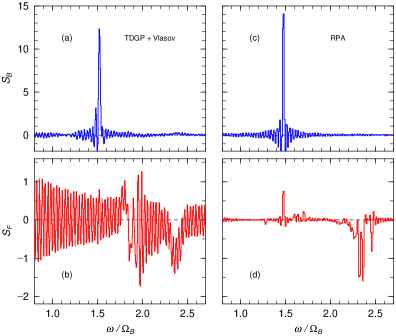
Figure 13: The strength functions of the quadrupole oscillations with the out-of-phase initial condition in ¹⁷⁰Yb$-^{173}$Yb  mixture (corresponding to Fig. 10); The panels and the lines are the same with Fig. 5.

Figure 19: Time evolution of the quadrupole oscillations in the ¹⁷⁴Yb$-^{173}$Yb mixture with the in-phase (a) and the out-of-phase (b) initial conditions in the time-interval $60<\tau<120$; the dashed and solid lines are for the boson and fermion oscillations, respectively.

References

- (1) S. Giorgini, L.P. Pitaevskii and S. Stringari, Rev. Mod. Phys. 80, 1215 (2008) and reference therein.
-
(2)
E.A. Cornell and C.E. Wieman, Rev. Mod. Phys. 74, 875 (2002);
W. Ketterle, Rev. Mod. Phys. 74, 1131 (2002). - (3) F. Dalfovo, et al., Rev. Mod. Phys. 71, 463 (1999).
- (4) C.J. Pethik and H. Smith, ”Bose-Einstein Condensation in Dilute Gases”, Cambridge University Press (2002).
- (5) J.O. Andersen, Rev. Mod. Phys. 76, 599 (2004).
-
(6)
A.G. Truscott, K.E. Streker, W.I. McAlexander,
G.B. Partridge and R.G. Hulet, Science 291, 2570 (2001);
G. Roati, F. Riboli, G. Modugno and M. Inguscio, Phys. Rev. Lett. 89, 150403 (2002). -
(7)
B. DeMarco and D.S. Jin, Science 285, 1703 (1999);
S.R. Granade, M.E. Gehm, K.M. OHara, J.E. Thomas, Phys. Rev. Lett. 88, 120405 (2002). - (8) F. Schreck, et al., Phys. Rev. Lett. 87, 080403 (2001).
-
(9)
A.G. Tuscott, K.E. Strecker, W.I. McAlexander, G.B. Parridge, and
R.G. Hullet, Science 291, 2570 (2001);
Z. Hadzibabic, et al., Phys. Rev. Lett. 88, 160401 (2002); ibid 91, 160401 (2003). - (10) M. Modugno, F. Ferlaino, F. Riboli, G. Roati, G. Modugno, M. Inguscio, Science 297, 2240 (2002); Phys. Rev. A 68, 043626 (2003).
- (11) H. Feshbach, Ann. Phys. (NY) 19, 287 (1962).
- (12) K. Mølmer, Phys. Rev. Lett. 80, 1804 (1998).
- (13) M. Amoruso, A. Minguzzi, S. Stringari, M. P. Tosi and L. Vichi, Eur. Phys. J. D 4, 261 (1998).
- (14) T. Miyakawa, K. Oda, T. Suzuki and H. Yabu, J. Phys. Soc. Japan 69, 2779 (2000).
- (15) M.J. Bijlsma, B.A. Heringa and H.T.C. Stoof, Phys. Rev. A 61, 053601 (2000).
- (16) L. Vichi, M. Inguscio, S. Stringari, and G.M Tino, Eur. Phys. J. D 11, 335 (2000).
- (17) L. Vichi, M. Inguscio, S. Stringari and G.M. Tino, J. Phys. B: At. Mol. Opt. Phys. 31 L899 (1998).
- (18) N. Nygaard and K. Mølmer, Phys. Rev. A 59, 2974 (1999).
- (19) X.X. Yi and C.P. Sun, Phys. Rev. A 64, 043608 (2001).
- (20) L. Viverit, C.J. Pethick and H. Smith, Phys. Rev. A 61, 053605 (2000).
- (21) P. Capuzzi and E.S. Hernández, Phys. Rev. A 66, 035602 (2002).
- (22) P. Capuzzi, A. Minguzzi and M.P. Tosi, Phys. Rev. A 68, 033605 (2003).
- (23) T. Miyakawa, T. Suzuki and H. Yabu, Phys. Rev. A 64, 033611 (2001).
- (24) R. Roth and H. Feldmeier, Phys. Rev. A 65, 021603(R) (2002).
- (25) P. Capuzzi and E. S. Hernández, Phys. Rev. A 64, 043607 (2001).
-
(26)
T. Sogo, T. Miyakawa, T. Suzuki and H. Yabu, Phys. Rev. A66, 013618 (2002);
T. Sogo, T. Suzuki and H. Yabu, Phys. Rev. A68, 063607 (2003). - (27) T. Miyakawa, K. Oda, T. Suzuki and H. Yabu, J. Phys. Soc. Jpn 69, 2779 (2000).
- (28) T. Miyakawa, T. Suzuki and H. Yabu, Phys. Rev. A 62, 063613 (2000).
- (29) A. Minguzzi and M.P. Tosi, Phys. Lett. A 268, 142 (2000).
- (30) S.K. Yip, Phys. Rev. A64, 023609 (2001).
- (31) T. Maruyama, H. Yabu and T. Suzuki, Phys. Rev. A72, 013609 (2005).
- (32) T. Maruyama, H. Yabu and T. Suzuki, Lazer Physics, 15, 656 (2005).
- (33) T. Maruyama and G.F. Bertsch, Phys. Rev. A77, 063611 (2008)
- (34) X.J. Liu and H. Hu, Phys. Rev. A67, 023613 (2003).
- (35) T. Maruyama and G.F. Bertsch, Phys. Rev. A73, 013610 (2006).
- (36) T. Maruyama and T. Nishimura, Phys. Rev. A75, 033611 (2007).
-
(37)
G.F. Bertsch, Nucl. Phys. A249, 253 (1975);
D.M. Brink and Leobardi, Nucl. Phys. A258, 285 (1976). -
(38)
G.F. Bertsch and K. Stricker, Phys. Rev. C13, 1312 (1976);
T. Suzuki, Prog. Theor. Phys. 64, 1627 (1980). - (39) F. Chevy, V. Bretin, P. Rosenbusch, K.W. Madison and J. Dalibard, Phys. Rev. Lett. 88, 250402 (2002).
- (40) M. Tohyama, Phys. Rev. A71, 043613 (2005).
-
(41)
T. Kimura, H. Saito and M. Ueda, J. Phys. Soc. Jpn. 68 (1999);
R. Graham and D. Walls, Phys. Rev. A57, 484 (1998);
D. Gorddon and C.M. Sarvage, Phys. Rev 85, 1440 (1999). -
(42)
D.S Jin, J.R. Ensher, M.R. Matthews, C.E. Wieman
and E.A. Cornell, Phys. Rev. Lett. 77, 420 (1996);
M.-O. Mewes et al., Phys. Rev. Lett. 77, 988 (1996). - (43) Y. Takasu, et al., Phys. Rev. Lett. 91, 040404 (2003).
- (44) T. Fukuhara, S. Sugawa, and Y. Takahashi, Phys. Rev. A76, 051604(R) (2007).
- (45) T. Fukuhara, Y. Takasu, M. Kumakura and Y. Takahashi, Phys. Rev. Lett. 98, 030401 (2007).
- (46) K. Enomoto, M. Kitagawa, K. Kasa, S. Tojo and Y. Takahashi, Phys. Rev. Lett. 98, 203201 (2007); M. Kitagawa, et al., Phys. Rev. A77, 012719 (2008).
- (47) L.P. Kadanoff and G. Baym, “Quantum Statistical Mechanics” (1962), New York.
-
(48)
R.W. Hockney AND J.W. Eastwood, ”Computer simulations using particles”,
McGraw-Hill, New York, 1981;
C.Y. Wong, Phys. Rev. C25, 1460 (1982). - (49) T. Maruyama and H. Yabu, in preparation.
- (50) B. Jackson and E. Zaremba, Phys. Rev. A66, 033606 (2002).
- (51) G.F. Bertsch and S. Das Gupta, Phys. Rep. 160 (1988) 189.
- (52) T. Maruyama, W. Cassing, U. Mosel, K. Weber, Nucl. Phys. A573, 653 (1994).