A Poissonian explanation for heavy tails in e-mail communication

Abstract

Patterns of deliberate human activity and behavior are of utmost importance in areas as diverse as disease spread, resource allocation, and emergency response. Because of its widespread availability and use, e-mail correspondence provides an attractive proxy for studying human activity. Recently, it was reported that the probability density for the inter-event time $\tau$ between consecutively sent e-mails decays asymptotically as $\tau^{-\alpha}$, with $\alpha\approx 1$. The slower than exponential decay of the inter-event time distribution suggests that deliberate human activity is inherently non-Poissonian. Here, we demonstrate that the approximate power-law scaling of the inter-event time distribution is a consequence of circadian and weekly cycles of human activity. We propose a cascading non-homogeneous Poisson process which explicitly integrates these periodic patterns in activity with an individual’s tendency to continue participating in an activity. Using standard statistical techniques, we show that our model is consistent with the empirical data. Our findings may also provide insight into the origins of heavy-tailed distributions in other complex systems.

The analysis of social and economic data has a long and illustrious history [1, 2, 3]. Despite their idiosyncratic complexity, a number of striking statistical regularities are known to describe individual and societal human behavior [4, 5, 6, 7]. These regularities are of enormous practical importance because they provide insight into how individual behaviors influence social and economic outcomes. Indeed, much of the current research on complex systems aims to quantify the impact of individual agents on the organization and dynamics of the system as a whole [8, 9]. Before we can predict how individuals affect, for example, the organization of systems, it is paramount to understand the behavior of the individual agents.

The current availability of digital records has made it much easier for researchers to quantitatively investigate various aspects of human behavior [10, 11, 12, 13, 14, 15, 16, 17, 18, 19, 20, 21]. In particular, e-mail communication records are attracting much attention as a proxy for quantifying deliberate human behavior due to the omnipresence of e-mail communication and availability of e-mail records [13, 14, 18, 16]. The data, however, does not provide a detailed record of all of the activities in which each individual participates; we do not know, for instance, when an individual is sleeping, eating, walking, or even browsing the web. The resulting uncertainty in deliberate human activity thus poses a fundamental challenge to quantifying and modeling human behavior.

Researchers commonly account for uncertainty or lack of information through stochastic models. One of the simplest stochastic models for human activity is a point process in which independent events occur at a constant rate $\rho$. Such processes are referred to as homogeneous Poisson processes, and they are used to describe a large class of phenomena, including some aspects of human activity [22]. Homogeneous Poisson processes have two well-known statistical properties: the time between consecutive events, the inter-event time $\tau$, follows an exponential distribution, $p(\tau)=\rho e^{-\rho\tau}$, and the number of events $N_{T}$ during a time interval of duration $T$ time units follows a Poisson distribution with mean $\rho T$.

Several recent studies of deliberate human activity, including e-mail correspondence, have focused on the former property. These studies have reported that the empirical distribution of inter-event times decays asymptotically as a power-law, $p(\tau)\propto\tau^{-\alpha}$, with exponent $\alpha\approx 1$ [23, 13, 14, 18]. Other studies have identified a similar power-law scaling in the inter-event time distribution of many other facets of human behavior, such as file downloads [10, 11, 12], letter correspondence [15, 17, 18], library usage [17], broker trades [17], web browsing [17, 19], human locomotor activity [20], and telephone communication [21]. These observations are in stark contrast with the predictions of a homogeneous Poisson process, suggesting that a more suitable null model with which to compare mechanistic models of human activity is a truncated power-law model with scaling exponent $\alpha=1$.

The heavy-tailed nature of the distribution of inter-event times prompts us to search for the mechanisms responsible for its emergence. Two main classes of mechanisms can be considered: (i) human behavior is primarily driven by rational decision making, which introduces correlations in activity thereby giving rise to heavy-tails; (ii) human behavior is primarily driven by external factors such as circadian and weekly cycles, which introduces a set of distinct characteristic time scales thereby giving rise to heavy-tails. While the former interpretation has been shown to give rise to a truncated power-law distribution of inter-event times, the latter has been rejected by some authors [17]. Indeed, even though Hidalgo [24] investigated a model with seasonal changes in activity rates that is able to generate data with an approximate power-law decay in the distribution of inter-event times with exponents $\alpha\approx 2$ or $\alpha\approx 1$, the $\alpha\approx 1$ case requires a specific relationship between the rates of activity $\rho_{i}$ and the corresponding duration of the seasons $T_{i}$ over which each rate holds. It has therefore been argued that seasonality alone can only robustly give rise to heavy-tailed inter-event time distributions with exponent $\alpha\approx 2$ [17].

Here, we demonstrate that the distribution of inter-event times in e-mail correspondence patterns display systematic deviations from the truncated power-law null model due to circadian and weekly patterns of activity. We subsequently propose a mechanistic model that incorporates these observed cycles, and a novel simulated annealing procedure to nonparametrically estimate its parameters. We then use Monte Carlo hypothesis testing to demonstrate that the predictions of our model are consistent with the observed heavy-tailed inter-event time distribution. Finally, we discuss the implications of our findings on modeling human activity patterns and, more generally, complex systems.

1 Empirical patterns

We study a database of e-mail records for 3,188 e-mail accounts at a European university over an 83-day period [23]. Each record comprises a sender identifier, a recipient identifier, the size of the e-mail, and a time stamp with a precision of one second. We preprocess the data set and identify a set of 394 accounts which provide enough data to quantify human activity and which are likely neither spammers nor listservs (see SI Sec. S1).

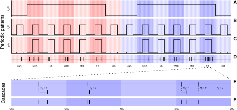
Figure 1: Example of a periodic and cascading stochastic process. A, Expected probability of starting an active interval during a particular day of the week $p_{w}(t)$. We depict two weeks to emphasize that this pattern is periodic and that every week is statistically identical to every other week. We surmise that e-mail users are more likely to send e-mails on the same days of the week, a consequence of regular work schedules. B, Expected probability of starting an active interval during a particular time of the day $p_{d}(t)$. Again, we depict 14 days to emphasize that this pattern is periodic and that every day is statistically identical to every other day. We surmise that e-mail users are more likely to send e-mails during the same times of the day, a consequence of circadian sleep patterns. C, The resulting activity rate $\rho(t)$ for the non-homogeneous Poisson process. The activity rate $\rho(t)$ is proportional to the product of the daily and weekly patterns of activity where the proportionality constant $N_{w}$ is the average number of active intervals per week (Eq. [1]). D, A time series of events generated by a non-homogeneous Poisson process. Each event in this time series initiates a cascade of additional events, an active interval. E, Schematic illustration of cascading activity. During cascades—active intervals—we expect that an individual will send $N_{a}$ additional e-mails according to a homogeneous Poisson process with rate $\rho_{a}$. We denote the start of active intervals with a dashed line to signify that the activity is no longer governed by the non-homogeneous Poisson process rate $\rho(t)$. Once the active interval concludes, e-mail usage is again governed by the periodic rate $\rho(t)$. We refer to the collection of active intervals as the active interval configuration $\mathcal{C}$ throughout the manuscript. F, Observed time series. Since the data does not isolate intervals of activity, the observed time series is the superposition of both the non-homogeneous Poisson process time series and the active interval time series.

In order to gain some intuition about e-mail activity patterns, let us consider a fictitious student, Katie. Katie arrives at the university 20 minutes before her Thursday morning class. During this time, she decides to check her e-mail and sends three e-mails. Katie checks her e-mail after lunch and sends a brief e-mail to a friend before her next class. Later that evening, Katie sends four more e-mails once she has finished her homework. Katie does not check her e-mail again until the following day when she sends e-mails intermittently between attending classes, completing homework assignments, and meeting social engagements. Katie spends the weekend without e-mail access and doesn’t send another e-mail until Monday. Katie’s e-mail activity, which is similar to many e-mail users, is both periodic and cascading. That is, there are periodic changes in her activity rate, which account for her sleep and work patterns, and there are cascades of activity—active intervals—of varying length when Katie primarily focuses on e-mail correspondence (Fig. 1).

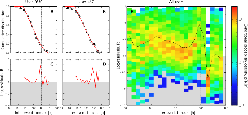
Figure 2: Systematic deviations of the data from the truncated power-law null model due to periodic patterns of human activity. The vertical lines at $\tau=10$ hours is meant as a guide to the eye. A–B, Comparison of truncated power-law model (red line) with empirical data ($\square$) for Users 2650 and 467 from the data set [23]. Lines of best fit are estimated by minimizing the area test statistic (see SI Sec. S4). C–D, Log-residual, $R=\ln(p_{\mathcal{M}}(\tau|\widehat{\theta})/p(\tau))$ of the best-fit truncated power-law distribution model $\mathcal{M}$. The shaded region denotes inter-event times where the null model underestimates the data. If the empirical inter-event time distribution were well-described by the truncated power-law null model, the log-residuals $R$ would be small and normally distributed, particularly in the tail of the distribution. However, the log-residuals $R$ have large systematic fluctuations in the tail of the inter-event time distribution ($\tau>0.25$ hours) where the power-law scaling approximately holds. E, Conditional probability density $p(R|\tau)$ obtained for all 394 users under consideration. The average log-residual at each inter-event time is represented by the dashed line. Both the average log-residual and conditional probability density indicate that nearly all users under consideration systematically deviate from the truncated power-law null model, as anticipated from the arguments in the main text.

If our intuition about deliberate human activity is correct, then the periodic patterns of activity should manifest itself in the inter-event time statistics, particularly when compared with the predictions of the truncated power-law null model which does not account for temporal periodicities (see SI Sec. S4). Specifically, we anticipate that e-mail users typically send e-mails during the same 8-hour periods of the day. We therefore expect the data to have significantly more inter-event times between $24\pm 8$ hours—the time required to send e-mails on consecutive workdays—than the truncated power-law model predictions. We therefore expect that the null model underestimates the number of inter-event times between 16 and 32 hours. Due to the normalization of the probability density, the truncated power-law model will over-estimate other inter-event times. These predictions are all confirmed by the data, suggesting that periodicity is a fundamental aspect of human activity (Fig. 2).

2 Model

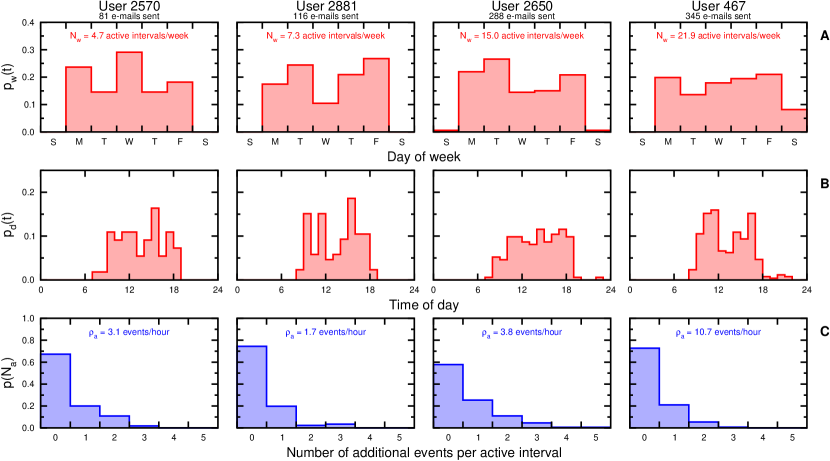
Figure 3: Patterns of e-mail activity for four users in increasing order of e-mail usage (see SI Fig. S7 for the same analysis for all 394 users). These e-mail users exemplify the e-mail usage patterns that are typical of the users in the data set. We use simulated annealing to identify active intervals and calculate the parameters for the cascading non-homogeneous Poisson process (see Methods). The red distributions and text (A–B) correspond with the parameters for the primary process, a non-homogeneous Poisson process, while the blue distributions and text (C) correspond with the parameters for the secondary process, a homogeneous Poisson process. A–B, Active intervals are much more likely during weekdays rather than weekends and during the daytime rather than the nighttime. These prolonged periods of inactivity lead to the heavy tail in the inter-event time distribution. C, Small inter-event times, in contrast, are characterized by active intervals. One can interpret active intervals in several ways: larger $\rho_{a}$ may indicate that a user is a more proficient e-mail user; larger $\langle N_{a}\rangle/\rho_{a}$ may suggest that an individual has a larger attention span; $N_{a}/\rho_{a}$ may be the time that an individual has to check e-mail before their next commitment.

We propose a model of e-mail usage that incorporates the hypothesized periodic and cascading features of human activity. We account for periodic activity with a primary process, which we model as a non-homogeneous Poisson process. Whereas a homogeneous Poisson process has a constant rate $\rho$, a non-homogeneous Poisson process has a rate $\rho(t)$ that depends on time. In our model, the rate $\rho(t)$ depends on time in a periodic manner; that is, $\rho(t)=\rho(t+W)$, where $W$ is the period of the process. Consistent with our observations (Fig. 3), we relate the rate of the non-homogeneous Poisson process to the daily and weekly distributions of active interval initiation, $p_{d}(t)$ and $p_{w}(t)$:

$$\rho(t) = N_{w}p_{d}(t)p_{w}(t),$$ (1)

where the period $W$ is one week and the proportionality constant $N_{w}$ is the average number of active intervals per week.

We further assume that each event generated from the primary process initiates a secondary process, which we model as a homogeneous Poisson process with rate $\rho_{a}$. We refer to these “cascades of activity” as active intervals, during which $N_{a}$ additional events occur where $N_{a}$ is drawn from some distribution $p(N_{a})$. Once the $N_{a}$ events have occurred in the active interval, the activity of the individual is again governed by the primary process defined by Eq. [1]. Our model thus mimics how individuals like Katie use e-mail: Katie sends e-mails sporadically throughout the day, but once she starts checking her e-mail, it is relatively easy to send additional e-mails in rapid succession. We refer to the resulting model as a cascading non-homogeneous Poisson process.

3 Results

To compare our model with the empirical data, we first need to estimate the parameters of our model from the data. Ideally, the data would specify which events belong to the same active intervals—the active interval configuration $\mathcal{C}$—so that we could estimate the distributions $p_{d}(t)$, $p_{w}(t)$, and $p(N_{a})$. The data we analyze, however, does not specify the actual active interval configuration $\mathcal{C}_{o}$ so it is not evident whether, for example, $p(N_{a})$ should be described by a normal or exponential distribution.

Because we do not know a priori the functional form of the activity pattern in the cascading process, we cannot use the formalism implemented by, for example, Scott and co-workers [34, 35]. Instead, we introduce a new method that enables us to nonparametrically infer the empirical distributions $p_{d}(t)$, $p_{w}(t)$, and $p(N_{a})$ from the data.

Given a particular active interval configuration $\mathcal{C}$, we can easily calculate all of our model’s parameters and compare it’s predictions with the empirical data: $N_{w}$ is the average number of active intervals per week; $p_{d}(t)$ and $p_{w}(t)$ are the probabilities of starting an active interval at a particular time of day and week respectively; the active interval rate $\rho_{a}$ is the inverse of the average inter-event time in active intervals; and the probability of $N_{a}$ additional events occurring during an active interval $p(N_{a})$ is estimated directly from the active interval configuration (Fig. 3). We then manipulate the active interval configuration $\mathcal{C}$ to find the active interval configuration $\widehat{\mathcal{C}}$ that gives a best estimate of the observed inter-event time distribution (see Methods). This method allows us to infer the best-estimate distributions $\widehat{p}_{d}(t)$, $\widehat{p}_{w}(t)$, and $\widehat{p}(N_{a})$ given the data and our proposed model without making any assumptions on their functional forms.

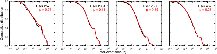
Figure 4: Comparison of the predictions of the cascading non-homogeneous Poisson process (red line) with the empirical cumulative distribution of inter-event times $P(\tau)$ (black line) for the same users from Fig. 3 (see SI Fig. S7 for the same analysis for all 394 users). We use the area test statistic $A$ (Eq. [2]) and Monte Carlo hypothesis testing to calculate the $p$-value between the model and the data (see SI Sec. S3). As these figures are presented, the area test statistic $A$ is the area between the two curves. Not only do the predictions of the cascading non-homogeneous Poisson process visually agree with the empirical data, but the $p$-values indicate that it can not be rejected as a model of e-mail activity at a conservative 5% significance level.

We next compare the predictions of the cascading non-homogeneous Poisson process with the empirical cumulative distribution of inter-event times $P(\tau)$ for all 394 users under consideration in the present study (see SI Fig. S7). Since we are using the empirical data to estimate the parameters for our model—that is, the estimated parameters depend on the data—we must use Monte Carlo hypothesis testing [29, 30] to assess the significance of the agreement between the predictions of our model and the empirical data (see SI Sec. S3). The visual agreement of our model’s predictions are confirmed by $p$-values clearly above our 5% rejection threshold (Fig. 4).

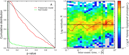
Figure 5: A, Summary of the hypothesis testing results for the cascading non-homogeneous Poisson process and the truncated power-law null model for the 394 users under consideration. For each user, we compute the $p$-value between their inter-event time distribution and the predictions of each model (see SI Sec. S3). We reject a model for a particular user if the $p$-value is less than the 5% rejection threshold (gray shaded region). At this significance level, the cascading non-homogeneous Poisson process can be rejected for one user while the truncated power-law null model can be rejected for 344 users (see SI Sec. S4). Note that if the data were actually generated by one of the models tested, we would expect to see a uniform distribution of $p$-values (dashed line). Since this is very nearly the case for the cascading non-homogeneous Poisson process, this provides additional evidence that our model is consistent with the data. B, Conditional probability density $p(R|\tau)$ obtained for all 394 users under consideration. The average log-residual at each inter-event time is represented by the dashed line. In contrast to the results in Fig. 2E, we find no systematic deviations between the model predictions and the data in the tail of the inter-event time distribution where the power-law scaling approximately holds.

In fact, the cascading non-homogeneous Poisson process can only be rejected at the 5% significance level for one user, indicating that our model can not be rejected as a model of human dynamics. By comparison, the truncated power-law null model is rejected at the 5% significance level for 344 users. Indeed, the null model is always rejected for many more users than the cascading non-homogeneous Poisson process regardless of the rejection threshold selected and our model displays none of the systematic deviations from the data observed for the truncated power-law null model (Fig. 5)

4 Discussion

Our results clearly demonstrate that circadian and weekly cycles, when coupled to cascading activity, can accurately describe the heavy-tails observed in email communication patterns. The question then is, would rational decision making together with circadian and weekly cycles be equally able to describe the statistical patterns observed for e-mail communication? Even if the answer to this question is affirmative, parsimony suggests that rational decision making is not a necessary component of human activity patterns, given our simpler explanation.

In addition to providing a good description of e-mail communication patterns, we surmise that our model is readily applicable to many other conscious human activities. For instance, most people make telephone calls sporadically throughout the day. After a telephone call has been made, it is effortless to make another telephone call. Similarly, individuals run errands throughout the month. Once an individual runs one errand, it is easier to run another errand during the same trip than it is to run errands again the following day. Both of these anecdotes are illustrative of the way humans tend to optimize their time and effort to accomplish the tasks in their daily routines, a process that is captured by the periodic and cascading mechanisms in our model.

The particular periodic and cascading features that are incorporated into our model depend on the activity under consideration. For instance, sexual activity is influenced by menstrual cycles [31] and airline travel is influenced by seasonality [32]. Furthermore, our model can also be generalized to cases in which the parameters are not stationary. This may be important, for instance, in the case of Darwin and Einstein’s letter correspondence in which the number of letters sent per year increases 100-fold over 40 years [15, 18].

Although our model is only designed to account for a single activity (e-mail correspondence), it can easily be extended to incorporate the multitude of activities in which any individual participates. To facilitate the inclusion of additional activities, it is useful to interpret our model as a non-stationary hidden Markov point process [33, 34]. Within this framework, an individual switches between any two activities $i$ and $j$ with some probability defined by a non-stationary Markov transition matrix $T_{ij}(t)$ which depends on time $t$. For instance, our model can be redefined as a non-stationary hidden Markov point process which switches between two states: a state in which an individual is not composing e-mails and a state in which an individual is composing e-mails. Predictions of models that incorporate more than one activity can then be verified against data that records several activities for a single individual.

Our model further suggests a novel experiment [36] which not only records when an individual has sent an e-mail, but also when that individual is using a computer or actively utilizing an e-mail client. This additional data would provide direct empirical evidence for describing active intervals. In the absence of such data, we have developed a simulated annealing procedure which allows us to nonparametrically infer the hidden Markov structure of our model, providing insight into how to compare our model with other cascading point processes [26, 27].

While our model provides an accurate description of when an e-mail is sent, a question left unaddressed is to determine whom the probable recipient of that e-mail is going to be. For instance, one might speculate that e-mails are sent randomly with some Poissonian rate to acquaintances or individuals which share common interests. Alternatively, it is plausible that e-mails are sent based on a perceived priority of important tasks, perhaps in response to previous correspondence [14]. When combined with our model that statistically describes when individuals send e-mails, quantifying the likely recipient of an e-mail will provide an important step toward describing how the structure of e-mail and social networks evolve.

Our study also provides a clear demonstration of how hypothesis testing [29, 37] can objectively assess the validity of a proposed model—a procedure we vehemently advocate. Using this methodology, we demonstrate that while both models reproduce the asymptotic scaling of the observed inter-event time distribution, our model is consistent with the entire inter-event time distribution whereas the truncated power-law null model is not.

The consequences of our findings are clear; demonstrating that a model reproduces the asymptotic power-law scaling of a distribution does not necessarily provide evidence that the model is an accurate mechanistic description of the underlying process. Indeed, there is mounting evidence that some purported power-law distributions in complex systems may not be power-laws at all [38, 39, 40]. There may be a common explanation for these apparent power-laws: complex systems are inherently hierarchical but the distinct levels in the hierarchy are difficult to distinguish [41]. In the case of e-mail correspondence for example, the active intervals are not recorded in the data data, thereby concealing the various scales of e-mail activity. This demonstrates how the mixture of scales of activity can give rise to scale-free activity patterns. We suspect that similar mixture-of-scales explanations [42, 43, 44, 45, 46] may provide a basis for the reported universality of heavy-tailed distributions in complex systems.

5 Methods

5.1 Area test statistic

We quantify the agreement between a model $\mathcal{M}(\theta)$ with parameters $\theta$ and data set $\mathcal{D}$ by measuring the area $A$ between the empirical cumulative distribution function $P_{\mathcal{D}}(u)$ and the model cumulative distribution function $P_{\mathcal{M}}(u|\theta)$:

$$A = \int\left|P_{\mathcal{D}}(u)-P_{\mathcal{M}}(u|\theta)\right|du.$$ (2)

We specify $u=\ln\tau$, which is roughly uniformly distributed, to improve the numerical efficiency of our simulated annealing procedure. The area test statistic is advantageous as it is easy to interpret and it retains more information about the distribution than many other test statistics (see SI Sec. S2).

5.2 Identifying active intervals

If we know the actual active interval configuration $\mathcal{C}_{o}$, it would be straightforward to compute the parameters $\theta_{o}=\{N_{w},p_{d}(t),p_{w}(t),\rho_{a},p(N_{a})\}$ of the cascading non-homogeneous Poisson process. The data, however, does not identify the actual active interval configuration $\mathcal{C}_{o}$, we must use heuristic methods (see SI Sec. S5) to determine the best-estimate active interval configuration $\widehat{\mathcal{C}}$, from which we can compute the best-estimate parameters $\widehat{\theta}$. We use simulated annealing to minimize the area test statistic $A$ (Eq. [2]) for the inter-event time distribution. Thus, identifying active intervals that are consistent with our expectations for our model reduces to finding the best-estimate active interval configuration $\widehat{\mathcal{C}}$ which minimizes the area $A$ between the empirical data and the predictions of the cascading non-homogeneous Poisson process.

Our simulated annealing procedure is as follows. Starting from a random active interval configuration $\mathcal{C}$ in which adjacent events are randomly assigned to the same active interval, we compute the parameters $\theta$ of the cascading non-homogeneous Poisson process, then we numerically estimate the cumulative distribution $P_{\mathcal{M}}(u|\theta)$, and finally we measure the area test statistic $A(\mathcal{C})$ of the active interval configuration $\mathcal{C}$. The active interval configuration is modified to a new configuration $\mathcal{C}^{\prime}$ by either merging two adjacent active intervals or by splitting an active interval. If the new configuration $\mathcal{C}^{\prime}$ reduces the area test statistic, then the new configuration is unconditionally accepted. Otherwise the configuration is conditionally accepted with probability $\exp(-(A(\mathcal{C}^{\prime})-A(\mathcal{C}))/T)$, where $T$ is the effective “temperature” measured in units of the area test statistic $A$. After attempting $2N$ configurations at each temperature so that each pair of $N$ consecutive events might be merged and split, we reduce the temperature $T$ by 5% until the active interval configuration settles at the best-estimate $\widehat{\mathcal{C}}$ without moving for 5 consecutive cooling stages. We have verified that our simulated annealing procedure accurately identifies active intervals and estimates parameters $\theta$ in synthetically generated cascading non-homogeneous Poisson process data sets (see SI Sec. S5 and Fig. S5).

- [1] Smith A (1786) An Inquiry into the Nature and Causes of the Wealth of Nations (Methuen & Co., London).
- [2] Pareto V (1906) Manuale di Economia Politica (Milano, Societa Editrice).
- [3] Zipf GK (1949) Human Behavior and the Principle of Least Effort: An Introduction to Human Ecology (Addison-Wesley Press, Cambridge, MA).
- [4] Stanley MHR, Amaral LAN, Buldyrev SV, Havlin S, Leschhorn H, Maass P, Salinger MA, Stanley HE (1996) Scaling behaviour in the growth of companies. Nature 379: 804–806.
- [5] Huberman BA, Pirolli PLT, Pitkow JE, Lukose RM (1998) Strong regularities in world wide web surfing. Science 280: 95–97.
- [6] Plerou V, Amaral LAN, Gopikrishnan P, Meyer M, Stanley HE (1999) Similarities between the growth dynamics of university research and of competitive economic activities. Nature 400: 433–437.
- [7] Amaral LAN, Ivanov PC, Aoyagi N, Hidaka I, Tomono S, Goldberger AL, Stanley HE, Yamamoto Y (2001) Behavioral-independent features of complex heartbeat dynamics. Phys Rev Lett 86: 6026–6029.
- [8] Newman MEJ (2003) The structure and function of complex networks. SIAM Review 45: 167–256.
- [9] Castellano C, Fortunato S, Loreto V (2007) Statistical physics of social dynamics arXiv:0710.3256.
- [10] Johansen A, Sornette D (2000) Download relation dynamics on the WWW following newspaper publication of URL. Physica A 276(1–2): 338–345.
- [11] Johansen A (2001) Response times of internauts. Physica A 296(3–4): 539–546.
- [12] Chessa AG, Murre JM (2004) A memory model for Internet hits after media exposure. Physica A 333(1): 541–552.
- [13] Johansen A (2004) Probing human response times. Physica A 338: 286–291.
- [14] Barabási AL (2005) The origin of bursts and heavy tails in human dynamics. Nature 435: 207–211.
- [15] Oliveira JG, Barabási AL (2005) Darwin and Einstein correspondence patterns. Nature 437: 1251.
- [16] Stouffer DB, Malmgren RD, Amaral LAN (2006) Log-normal statistics in e-mail communication patterns arXiv:physics/060527.
- [17] Vázquez A, Oliveira JG, Dezsõ Z, Goh KI, Kondor I, Barabási AL (2006) Modeling bursts and heavy tails in human dynamics. Phys Rev E 73(3): 036127.
- [18] Vázquez A (2006) Impact of memory on human dynamics. Physica A 373: 747–752.
- [19] Dezsõ Z, Almaas E, Lukács A, Rácz B, Szakadát I, Barabási AL (2006) Dynamics of information access on the web. Phys Rev E 73: 066132.
- [20] Nakamura T, Kiyono K, Yoshiuchi K, Nakahara R, Struzik ZR, Yamamoto Y (2007) Universal scaling law in human behavioral organization. Phys Rev Lett 99: 138103.
- [21] Candia J, González MC, Wang P, Schoenharl T, Madey G, Barabási AL (2007) Uncovering individual and collective human dynamics from mobile phone records. J Phys A 41: 224015.
- [22] Daley DJ, Vere-Jones D (1988) An Introduction to the Theory of Point Processes (Springer-Verlag).
- [23] Eckmann JP, Moses E, Sergi D (2004) Entropy of dialogues creates coherent structure in e-mail traffic. Proc Natl Acad Sci USA 101: 14333–14337.
- [24] Hidalgo C (2006) Conditions for the emergence of scaling in the inter-event time of uncorrelated and seasonal systems. Physica A 369(2): 877–883.
- [25] Eckmann JP (2008). Private communication.
- [26] Neyman J, Scott EL (1958) A statistical approach to problems of cosmology. J Roy Stat Soc B 20: 1–43.
- [27] Lowen SB, Teich MC (2005) Fractal-Based Point Processes (John Wiley & Sons, Inc.).
- [28] Hawkes AG (1971) Spectra of some self-exciting and mutually exciting point processes. Biometrika 58(1): 83–90.
- [29] D’Agostino RB, Stephens MA (1986) Goodness-of-Fit Techniques (Marcel Kekker, Inc.).
- [30] Press WH, Teukolsky SA, Vetterling WT, Flannery BP (2002) Numerical Recipes in C: The Art of Scientific Computing (Cambridge University Press, New York), 2nd ed.
- [31] Udry J, Morris NM (1968) Distribution of coitus in the menstrual cycle. Nature 220: 593–596.
- [32] Kulendran N, King ML (1997) Forecasting international quarterly tourist flows using error-correction and time-series models. J Int Forecasting 13: 319–327.
- [33] Elliott RJ, Aggoun L, Moore JB (1995) Hidden Markov Models: Estimation and Control (Springer-Verlag).
- [34] Scott SL (1999) Bayesian analysis of a two-state Markov modulated Poisson process. J Comput Graph Stat 8(3): 662–670.
- [35] Scott SL, Smyth P (2003) in Bayesian Statistics 7 (Oxford University Press).
- [36] Watts DJ (2007) A twenty-first century science. Nature 445: 489.
- [37] Sivia DS, Skilling J (2006) Data Analysis: A Bayesian Tutorial (Oxford Science Publications).
- [38] Perline R (2005) Strong, weak and false inverse power laws. Stat Sci 20(1): 68–88.
- [39] Edwards AM, Phillips RA, Watkins NW, Freeman MP, Murphy EJ, Afanasyev V, Buldyrev SV, da Luz M, Raposo E, Stanley H, Viswanathan GM (2007) Revisiting Lévy flight search patterns of wandering albatrosses, bumblebees and deer. Nature 449: 1044–1048.
- [40] Clauset A, Shalizi CR, Newman MEJ (2007) Power-law distributions in empirical data arXiv:0706.1062.
- [41] Sales-Pardo M, Guimerà R, Moreira AA, Amaral LAN (2007) Extracting the hierarchical organization of complex systems. Proc Natl Acad Sci U S A 104: 15224–15229.
- [42] Silcock H (1954) The phenomenon of labour turnover. J Roy Stat Soc A 117(4): 429–440.
- [43] Harris CM (1968) The Pareto distribution as a queue service discipline. Oper Res 16(2): 307–313.
- [44] Hausdorff JM, Peng C (1996) Multiscaled randomness: A possible source of noise in biology. Phys Rev E 54(2): 2154.
- [45] Willinger W, Govindan R, Jamin S, Paxson V, Shenker S (2002) Scaling phenomena in the Internet: critically examining criticality. Proc Natl Acad Sci USA 99: 2573–2580.
- [46] Motter AE, de Moura APS, Grebogi C, Kantz H (2005) Effective dynamics in Hamiltonian systems with mixed phase space. Phys Rev E 71: 036215.