Product Structures for Legendrian Contact Homology

Abstract.

Legendrian contact homology (LCH) and its associated differential graded algebra are powerful non-classical invariants of Legendrian knots. Linearization makes the LCH computationally tractable at the expense of discarding nonlinear (and noncommutative) information. To recover some of the nonlinear information while preserving computability, we introduce invariant cup and Massey products — and, more generally, an $A_{\infty}$ structure — on the linearized LCH. We apply the products and $A_{\infty}$ structure in three ways: to find infinite families of Legendrian knots that are not isotopic to their Legendrian mirrors, to reinterpret the duality theorem of the fourth author in terms of the cup product, and to recover higher-order linearizations of the LCH.

1. Introduction

A central problem in the theory of Legendrian knots in the standard contact $3$-space is to produce effective invariants and understand their geometric meaning. The first “classical” invariants of Legendrian knots were the Thurston-Bennequin and rotation numbers [1]. These two invariants classify Legendrian knots in the standard contact structure when the underlying smooth knot type is the unknot [7], a torus knot, or the figure eight knot [9]; see also [4].

These early results raised the question of whether non-isotopic Legendrian knots with the same classical invariants exist. A particular instance of this question was Fuchs and Tabachnikov’s Legendrian mirror question [13]: given a Legendrian knot $K$ with rotation number zero, is it isotopic to its image $\overline{K}$ under the contactomorphism $(x,y,z)\mapsto(x,-y,-z)$? This map is isotopic to the identity through diffeomorphisms but not contactomorphisms (it changes the sign of the contact form). New invariants, beginning with Legendrian contact homology [2, 6] and followed by normal rulings [3] and the Knot Floer Homology Legendrian invariant [23], have been used to find non-isotopic Legendrian knots with the same classical invariants. In this paper, we study the algebraic structure of the Legendrian contact homology differential graded algebra (DGA) and how it can be used to define computable invariants of Legendrian knots that are stronger that Chekanov’s linearization and that detect the geometric property of a Legendrian knot not being isotopic to its Legendrian mirror.

The Legendrian contact homology of a Legendrian knot $K$ is the homology of a free non-commutative DGA $(\mathcal{A}_{K},\partial)$ over $\mathbb{Z}_{2}$ whose differential is nonlinear, so it is extremely hard to exploit directly. Several methods have been devised to extract useful information from the DGA. The most tractable of these is Chekanov’s method of linearization, which uses an “augmentation” $\varepsilon:\mathcal{A}_{K}\to\mathbb{Z}_{2}$ to produce a finite-dimensional chain complex whose homology is denoted $LCH^{\varepsilon}_{*}(K)$ [2]. The loss of noncommutative structure, however, means that linearized homology is unable to detect any differences between a Legendrian knot and its mirror; this is also true of another easily computable invariant, a normalized count of augmentations [22]. Chekanov also defined higher-order linearizations that take nonlinear parts of the differential into account, but these have not yet proved to be any more effective than the original (order one) linearization. Still another method, Ng’s characteristic algebra, retains the nonlinear structure of the DGA and can be used to distinguish a Legendrian $6_{2}$ knot from its mirror [21], but its practical use is more art than algorithm.

In this paper, we develop a new method of extracting nonlinear information from the DGA, namely by defining cup and Massey product structures — and even $A_{n}$ and $A_{\infty}$ structures — on the linearized cohomology $LCH^{*}_{\varepsilon}(K)$. The cup product has already appeared implicitly in the fourth author’s investigation of duality for the linearized contact homology [27], and we reinterpret duality in terms of the cup product in Section 4.2. Though interesting structurally, the cup products that generate the duality pairing are of no use as invariants. There exist knots, however, with nontrivial — and noncommutative — cup products that do not contribute to the duality pairing. In fact, all of the product structures produce nontrivial invariants.

Theorem 1.1.

There exists an infinite family of knots that are distinguished from their Legendrian mirrors by their linearized cohomology rings. More generally, for each $n>2$, there exists an infinite family of knots that are distinguished from their Legendrian mirrors by their $n^{th}$-order Massey products but not by their $k^{th}$ order Massey products for all $k<n$.

Further, the product structures incorporate all of the information (and more) from Chekanov’s higher-order linearizations.

Theorem 1.2.

For all $n>1$, the $A_{n}$ structure on $LCH^{*}_{\varepsilon}(K)$ is strictly stronger than the order $n$ linearized contact (co)homology.

Finally, we can reinterpret a result of the fourth coauthor [27] in terms of the cup product operation.

Theorem 1.3.

For every Legendrian knot $K$ in the standard tight contact structure on $\mathbb{R}^{3}$ and every augmentation $\varepsilon$ of its contact homology DGA, there is an element $\kappa\in LCH^{\varepsilon}_{1}(K)$ and an element $c\in LCH^{1}_{\varepsilon}(K)$ such that $\langle c,\kappa\rangle=1$ and the pairing

$$\overline{LCH}_{\varepsilon}^{k}\otimes\overline{LCH}_{\varepsilon}^{-k}\to\mathbb{Z}_{2}:[a]\otimes[b]\mapsto\langle[a]\cup[b],\kappa\rangle$$

is symmetric and non-degenerate, where $\overline{LCH}_{\varepsilon}^{*}$ is a complement of the span of $c$.

We leave as open problems whether or not the Massey product structure on $LCH^{*}_{\varepsilon}(K)$ determines the third order linearized contact (co)homology and whether or not the higher order linearized contact (co)homologies are stronger invariants than the (first order) linearized contact (co)homology.

The rest of the paper is organized as follows: after reviewing some basic definitions in Section 2, we define the $A_{\infty}$ and product structures in Section 3. We show that the product structures are effective invariants in Section 4 by proving Theorem 1.1. We also establish Theorem 1.3 in this section. Finally, we prove Theorem 1.2 in Section 5.

Acknowledgements: The authors thank Jim Stasheff for several helpful discussions. The first author was supported by an REU program funded by the Georgia Institute of Technology. The second author was partially supported by NSF grants DMS-0804820. The third and fifth authors were supported as undergraduate summer research students by the Haverford College faculty support fund.

2. Background and Notation

We refer the reader to the survey article [8] or the first chapter of the text [25] for the basic notions of Legendrian knot theory. In particular, we assume that the reader is familiar with the Lagrangian ($xy$) and front ($xz$) projections (and the resolution procedure that generates a Lagrangian projection from a front projection by smoothing left cusps, turning right cusps into loops, and making all crossings be of the form in Figure 1) of a Legendrian knot in the standard contact $(\mathbb{R}^{3},\xi_{0}=\ker\alpha_{0})$.

2.1. Legendrian Contact Homology

In this section, we sketch the definition of Legendrian contact homology, which is the homology of the Chekanov-Eliashberg differential graded algebra (DGA). See Chekanov’s original paper [2], the paper [10], or the expository works [8, 25] for more details.

To define the Chekanov-Eliashberg DGA $(\mathcal{A}_{K},\partial)$ of a Legendrian knot $K$, we begin with the underlying algebra $\mathcal{A}_{K}$. Number the crossings of the Lagrangian projection of $K$ from $1$ to $n$, and let $A$ be the vector space over $\mathbb{Z}_{2}$ generated by the labels $\{q_{1},\ldots,q_{n}\}$. Define the algebra $\mathcal{A}_{K}$ to be the unital tensor algebra over $A$, i.e.,

(2.1) $$\mathcal{A}_{K}=\bigoplus_{k=0}^{\infty}A^{\otimes k}.$$

We sometimes denote $\mathcal{A}_{K}$ as $\mathcal{A}(q_{1},\ldots,q_{n})$ when we want to emphasize the generating set for the algebra.

The generators $q_{i}$ are graded by a Conley-Zehnder index that takes values in $\mathbb{Z}_{2r(K)}$; the grading then extends naturally to all of $\mathcal{A}_{K}$. Specifically, assume that at all crossings of $\pi_{l}(K)$, the strands meet orthogonally. Given a generator $q_{i}$, choose a path $\gamma_{i}$ inside $\pi_{l}(K)$ that starts on the overcrossing at $i$ and ends at the undercrossing. Then define the grading $|q_{i}|$ to be:

(2.2) $$|q_{i}|\equiv 2r(\gamma_{i})-\frac{1}{2}\mod 2r(K).$$

Finally, we need to define the differential $\partial$ on the generators of $\mathcal{A}_{K}$; it extends to the full algebra via linearity and the Liebniz rule. First, decorate the sectors near every crossing of $\pi_{l}(K)$ with positive and negative signs — called Reeb signs — as in Figure 1(a). To find $\partial q_{i}$, let $\Delta(q_{i})$ be the set of immersed disks (modulo smooth reparametrization) whose boundary lies in $\pi_{l}(K)$. Further stipulate that the disks have convex corners (see Figure 1(b)) such that the corner covers a positive Reeb sign at the crossing $i$ and negative Reeb signs at all other corners (it is possible that there are no other corners). Finally, each disk in $\Delta(q_{i})$ contributes a term to $\partial q_{i}$ consisting of the product of the generators associated to its negative corners, taken in counterclockwise order starting after $i$. Note that the DGA $(\mathcal{A}_{\overline{K}},\partial)$ for the Legendrian mirror $\overline{K}$ has the same generators as those for $K$, but the order of each term in the differential is reversed.

$-$$+$$+$$-$

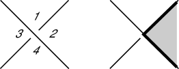
Figure 1. (a) The Reeb signs near a crossing of $\pi_{l}(K)$. (b) A convex corner.

That this definition produces an invariant of Legendrian knots was proven by Chekanov.

Theorem 2.1 (Chekanov [2]).

The differential $\partial$ has degree $-1$ and satisfies $\partial^{2}=0$. The Legendrian contact homology $H_{*}(\mathcal{A}_{K},\partial)$ is invariant under Legendrian isotopy.

In fact, Chekanov proved something more subtle: the “stable tame isomorphism” class of $(\mathcal{A}_{K},\partial)$ is an invariant. We recall the definition of stable tame isomorphism as it will be used below.

A graded chain isomorphism

$$\phi:\mathcal{A}(q_{1},...,q_{n})\longrightarrow\mathcal{A}(q^{\prime}_{1},\ldots,q^{\prime}_{n})$$

is elementary if there is some $j\in\{1,\ldots,n\}$ such that

(2.3) $$\phi(q_{i})=\begin{cases}q^{\prime}_{i},&i\neq j\\ q^{\prime}_{j}+u,&i=j\text{ where }u\in\mathcal{A}(q^{\prime}_{1},\ldots,q^{\prime}_{j-1},q^{\prime}_{j+1},\ldots,q^{\prime}_{n}).\end{cases}$$

A composition of elementary isomorphisms is called tame. The degree $i$-stabilization $S_{i}(\mathcal{A}(q_{1},\ldots,q_{n}))$ of $\mathcal{A}(q_{1},\ldots,q_{n})$ is defined to be $\mathcal{A}(q_{1},\ldots,q_{n},e^{i}_{1},e^{i}_{2})$. The grading and the differential are inherited from the original algebra and by setting $|e_{1}|=i$, $|e_{2}|=i-1$, $\partial e_{1}=e_{2}$, and $\partial e_{2}=0$.

Two differential algebras $(\mathcal{A},\partial)$ and $(\mathcal{A}^{\prime},\partial^{\prime})$ are stably tame isomorphic if after each algebra has been stabilized some number of times they become tame isomorphic by a map that is also a chain map.

2.2. Linearized Contact Homology and Cohomology

As it stands, it is difficult to use Legendrian contact homology in practical applications, as it is the homology of an infinite dimensional noncommutative algebra with a nonlinear differential. To find a more amenable invariant, we use Chekanov’s linearization technique. To do this, we break up the differential on $A$ into its components:

(2.4) $$\partial_{k}:A\to A^{\otimes k}.$$

If it were true that the constant term of the differential vanished, i.e. if $\partial_{0}=0$, then the fact that $\partial^{2}=0$ would imply that $\partial_{1}^{2}=0$. In particular, if $\partial_{0}=0$, then $(A,\partial_{1})$ is a finite-dimensional chain complex with easily computable homology.

It is rarely true, however, that $\partial_{0}=0$. To remedy this situation, consider graded algebra maps $\varepsilon:\mathcal{A}_{K}\to\mathbb{Z}_{2}$ that satisfy:

1. $\varepsilon(1)=1$, and

2. $\varepsilon\circ\partial=0$.

These maps are called augmentations. They do not always exist — see, for example, [12, 24, 26] — but when they do, they allow us to linearize the Chekanov-Eliashberg DGA. To see how, consider the graded isomorphism $\phi^{\varepsilon}:\mathcal{A}_{K}\to\mathcal{A}_{K}$ defined by $\phi^{\varepsilon}(q_{i})=q_{i}+\varepsilon(q_{i})$. This map defines a new differential $\partial^{\varepsilon}=\phi^{\varepsilon}\partial(\phi^{\varepsilon})^{-1}$; it is easy to check that $\partial^{\varepsilon}_{0}=0$. Thus, for each augmentation $\varepsilon$ of $(\mathcal{A}_{K},\partial)$, there is a chain complex $(A,\partial^{\varepsilon}_{1})$. This is called the linearized chain complex with respect to $\varepsilon$. There is also a cochain complex $(A^{*},\delta^{\varepsilon})$, where $A^{*}$ has a basis $\{p_{1},\ldots,p_{n}\}$ that is dual to $\{q_{1},\ldots,q_{n}\}$ and $\delta^{\varepsilon}$ is the adjoint of $\partial^{\varepsilon}_{1}$. The homologies of these complexes are called the linearized contact (co)homologies and are denoted by $LCH^{\varepsilon}_{*}(K)$ and $LCH_{\varepsilon}^{*}(K)$.

Chekanov extended the definition of the linearized (co)chain complex to include higher-order pieces of the differential. The $n^{\text{th}}$-order linearized chain complex with respect to $\varepsilon$ is given by the graded vector space of chains

$$A_{(n)}=\bigoplus_{i=1}^{\infty}A^{\otimes i}/\bigoplus_{i=n+1}^{\infty}A^{\otimes i}$$

together with the differential $\partial^{\varepsilon}_{(n)}$ induced from the quotient. Notice that $\partial^{\varepsilon}$ does indeed descend to the quotient since $\partial^{\varepsilon}_{0}=0$, so $\partial^{\varepsilon}$ cannot decrease the length of a tensor. The $n^{\text{th}}$-order cochain complex is defined by taking duals and adjoints, as usual. The homologies of these complexes are called the $n^{\text{th}}$-order linearized contact (co)homologies and are denoted by $LCH^{\varepsilon}_{*}(K,n)$ and $LCH_{\varepsilon}^{*}(K,n)$.

Chekanov proved that the set of all linearized (co)homologies taken over all possible augmentations is a Legendrian knot invariant; this set is called the linearized (co)homology invariant of $K$. Invariance also holds for the higher order linearized homologies.

Remark 2.2.

The proof relies on two facts that were proved in [2]: first, the linearized invariant does not change under stabilizations of the Chekanov-Eliashberg DGA. Second, given a tame isomorphism $\psi:(\mathcal{A},\partial)\to(\mathcal{A}^{\prime},\partial^{\prime})$ and an augmentation $\varepsilon^{\prime}$ of $(\mathcal{A}^{\prime},\partial^{\prime})$, the composite map $\phi^{\varepsilon^{\prime}}\psi$ factors as $\overline{\psi}\phi^{\varepsilon}$, where $\varepsilon$ is an augmentation of $\mathcal{A}$ and $\overline{\psi}$ does not reduce the lengths of words in $\mathcal{A}$. The map $\overline{\psi}$ is a DGA isomorphism between $(\mathcal{A},\partial^{\varepsilon})$ and $(\mathcal{A}^{\prime},(\partial^{\prime})^{\varepsilon^{\prime}})$, and hence restricts to an isomorphism between the linearized complexes $(A,\partial^{\varepsilon}_{1})$ and $(A^{\prime},(\partial^{\prime})^{\varepsilon^{\prime}}_{1})$.

3. $A_{\infty}$-algebras and Product Structures

As mentioned in the introduction, invariant product structures can be defined on the linearized cohomology invariant by using higher-order terms in the differential $\partial$. In fact, we shall see that the linearized cochain complex carries the structure of an $A_{\infty}$ algebra, and that the $A_{\infty}$ structure on the cochain complex induces an invariant $A_{\infty}$ structure on the linearized contact cohomology.

3.1. $A_{\infty}$ Algebras and Massey Products

An $A_{n}$-algebra over $\mathbb{Z}_{2}$ is a graded vector space $V$ over $\mathbb{Z}_{2}$ together with a sequence of graded maps $\mathbf{m}=\{m_{k}:V^{\otimes k}\to V\}_{1\leq k\leq n}$ of degree $1$ satisfying:

(3.1) $$\sum_{i+j+k=l}m_{i+1+k}\circ(1^{\otimes i}\otimes m_{j}\otimes 1^{\otimes k})=0$$

for all $1\leq l\leq n$. An $A_{\infty}$-algebra is the obvious generalization to an infinite sequence of maps. An $A_{\infty}$-algebra structure induces $A_{n}$ structures for all $n\geq 1$. Notice that Equation (3.1) for $l=1$ is $m_{1}\circ m_{1}=0,$ which implies that $m_{1}$ is a co-differential on $V$. From now on, we denote it by $\delta$. The cohomology of $(V,\delta)$ is denoted $H^{*}(V).$ When we take $l=2$ in Equation (3.1), we get:

$$\delta m_{2}(a,b)=m_{2}(\delta a,b)+m_{2}(a,\delta b)$$

for all $a,b\in V.$ Thus, $m_{2}$ descends to a well defined product $\mu_{2}$ on $H^{*}(V)$. We see this product is associative using Equation (3.1) when $l=3$:

(3.2) $$m_{2}(a,m_{2}(b,c)) +m_{2}(m_{2}(a,b),c)=\delta m_{3}(a,b,c)$$

$$+m_{3}(\delta a,b,c)+m_{3}(a,\delta b,c)+m_{3}(a,b,\delta c).$$

Thus, given an $A_{\infty}$ algebra $(V,\mathbf{m})$, we obtain an ordinary associative algebra $(H^{*}(V),\mu_{2})$.

Remark 3.1.

Usually, the $A_{\infty}$ algebra map $m_{k}$ is taken to have degree $2-k$ instead of degree $1$. Our maps $m_{k}$ should be thought of as degree $1$ maps on the suspension $A^{*}=SV$ induced by degree $2-k$ maps $\widetilde{m}_{k}$ defining a conventionally-graded $A_{\infty}$ algebra $(V,\widetilde{\bf{m}})$. Similar comments apply to the definition of $A_{\infty}$ morphisms, which are usually taken to have degree $n-1$ instead of degree $0$.

If we try to define a full $A_{\infty}$ structure on $H^{*}(V)$ by simply letting the maps $m_{k}$ descend to cohomology, we run into trouble already at $k=3$, as Equation (3.2) shows that $m_{3}(a,b,c)$ is not necessarily a cycle even if $a$, $b$, and $c$ are. We can proceed in one of two ways: first, following Stasheff [29], we can (partially) define a triple product on $H^{*}(V)$ as follows: given $[a],[b],[c]\in H^{*}(V)$, suppose that $\mu_{2}([a],[b])=[0]=\mu_{2}([b],[c])$. Let $\delta x=m_{2}(a,b)$ and let $\delta y=m_{2}(b,c)$. Then we see that

$$m_{3}(a,b,c)+m_{2}(a,y)+m_{2}(x,c)$$

is a cocycle. Since $x$ and $y$ are only defined up to the addition of cocycles, we get a well-defined element

$$\{[a],[b],[c]\}\in\tilde{H}^{*}(V)=\frac{H^{*}(V)}{\operatorname{Im}(\mu_{2}([a],\cdot))+\operatorname{Im}(\mu_{2}(\cdot,[c]))}.$$

This triple product is called a Massey product.

It is possible to inductively define higher-order Massey products on $H^{*}(V)$ using the $A_{\infty}$ structure. Given $[a_{1}],\ldots,[a_{n}]\in H^{*}(V)$, suppose that the product $\{[a_{i}],\ldots,[a_{j}]\}$ is defined and equal to zero modulo the successive images of all lower-order Massey products for all $1\leq i<j\leq n$. Following the order $3$ case in [29], we define:

$$\{[a_{1}],\ldots,[a_{n}]\}=\left[\sum_{k=2}^{n}\sum_{0\leq i_{1}<\cdots<i_{k-1}<n}m_{k}(b_{1,i_{1}},b_{i_{1}+1,i_{2}},\ldots,b_{i_{k-1}+1,n})\right],$$

where $b_{lm}\in V$ has been inductively defined by:

$$[b_{mm}] =[a_{m}],$$

$$\delta b_{lm} =\sum_{k=2}^{m-l+1}\sum_{l\leq i_{1}<\cdots<i_{k-1}<m}m_{k}(b_{l,i_{1}},b_{i_{1}+1,i_{2}},\ldots,b_{i_{k-1}+1,m}).$$

It is straightforward but tedious to check using the definition of the $b_{km}$ and the defining $A_{\infty}$ equation (3.1) that the higher-order Massey product is indeed a cocycle and is well-defined modulo the successive images of the lower-order Massey products in $H^{*}(V)$.

The Massey products have the practical advantage of computability, as we shall see, but the theoretical disadvantage of being only partially defined. The second way forward is to try to define a full $A_{\infty}$ structure on $H^{*}(V)$. To do this, we need the notion of a morphism of $A_{\infty}$-algebras; there are obvious analogs for $A_{n}$ algebras, and any $A_{\infty}$ morphism induces $A_{n}$ morphisms for all $n\geq 1$. An $A_{\infty}$ morphism $\boldsymbol{\phi}:(V,\mathbf{m})\to(W,\mathbf{n})$ is a collection of degree $0$ linear maps $\phi_{n}:V^{\otimes n}\to W$ that satisfy

(3.3) $$\sum_{i+j+k=n}\phi_{i+1+k}\circ(1^{\otimes i}\otimes m_{j}\otimes 1^{\otimes k})=\sum_{\begin{subarray}{c}1\leq r\leq n\\ i_{1}+\ldots+i_{r}=n\end{subarray}}n_{r}\circ(\phi_{i_{1}}\otimes\cdots\otimes\phi_{i_{r}}).$$

Notice that this equation implies that $\phi_{1}:V\to W$ commutes with the codifferentials on $V$ and $W$, and hence induces a map on cohomology. The morphism $\boldsymbol{\phi}$ is called an $A_{\infty}$ quasi-isomoprhism if $\phi_{1}$ induces an isomorphism on the cohomology.

Equation (3.3) for $n=2$ says that

$$\phi_{1}\circ m_{2}+\phi_{2}(\delta\otimes 1+1\otimes\delta)=n_{2}\circ(\phi_{1}\times\phi_{1})+\delta\circ\phi_{2}.$$

Thus, on the level of cohomology,

$$\phi_{1}m_{2}([a],[b])=m_{2}(\phi_{1}[a],\phi_{1}[b]).$$

In other words, $\phi_{1}$ preserves the product structure on cohomology. One may easily check that Equation (3.3) for $n>2$ implies that $\phi_{1}$ will preserve the Massey product and higher order product structures on the cohomology as well.

We now return to the discussion of defining an $A_{\infty}$ structure on $H^{*}(V)$. The relevant result is the Minimal Model Theorem, which we shall discuss in more detail in Section 5.

Theorem 3.2 (Kadeishvili [14]).

If $(V,\mathbf{m})$ is an $A_{\infty}$ algebra over a field, then its homology $H^{*}(V)$ also possesses an $A_{\infty}$ structure $\boldsymbol{\mu}$ such that $\mu_{1}=0$, $\mu_{2}$ is induced from $m_{2}$ as described above, and there exists an $A_{\infty}$ quasi-isomorphism $\boldsymbol{\phi}:(H^{*}(V),\boldsymbol{\mu})\to(V,\mathbf{m})$. The $A_{\infty}$ structure on $H^{*}(V)$ is unique up to $A_{\infty}$ quasi-isomorphism.

3.2. The $A_{\infty}$ Structure on the Linearized Cochain Complex

The reason for discussing $A_{\infty}$-algebras is the following proposition.

Proposition 3.3.

For each augmentation $\varepsilon$, the Legendrian contact homology DGA $(\mathcal{A},\partial)$ induces an $A_{\infty}$ structure on the linearized cochain complex $(A^{*},\delta^{\varepsilon})$.

Proof.

Denote by $m^{\varepsilon}_{k}$ the adjoint of $\partial^{\varepsilon}_{k}:A\to A^{\otimes k}$ for $k\geq 1$. Expanding the equation $(\partial^{\varepsilon})^{2}=0$ using $\partial^{\varepsilon}=\sum\partial^{\varepsilon}_{i}$ and looking at the term with image in $A^{\otimes n}$ gives:

$$\sum_{i+j+k=n}(1^{\otimes i}\otimes\partial^{\varepsilon}_{j}\otimes 1^{\otimes k})\circ\partial^{\varepsilon}_{i+1+k}=0.$$

Dualizing yields Equation (3.1). That $m^{\varepsilon}_{k}$ has degree $1$ follows from the fact that $\partial^{\varepsilon}_{k}$ has degree $-1$. ∎

Example 3.4.

Let $K$ be the Legendrian trefoil shown in Figure 2.

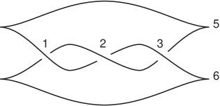
$b_{1}$$b_{2}$$b_{3}$$a_{1}$$a_{2}$

Figure 2. Legendrian right handed trefoil knot.

We label the Reeb chords $a_{1},a_{2},b_{1},b_{2}$ and $b_{3}$ as shown in the figure. One may easily compute that $|a_{i}|=1$ and $|b_{i}|=0.$ In addition, we have:

$$\partial a_{1} =1+b_{1}+b_{3}+b_{1}b_{2}b_{3}$$

$$\partial a_{2} =1+b_{1}+b_{3}+b_{3}b_{2}b_{1}$$

$$\partial b_{i} =0.$$

There are five different augmentations of this differential graded algebra; let us consider the augmentation $\varepsilon$ that sends $b_{3}$ to $1$ and all other generators to $0$. The augmented differential is:

$$\partial^{\varepsilon}a_{1} =b_{1}+b_{3}+b_{1}b_{2}+b_{1}b_{2}b_{3}$$

$$\partial^{\varepsilon}a_{2} =b_{1}+b_{3}+b_{2}b_{1}+b_{3}b_{2}b_{1}$$

$$\partial^{\varepsilon}b_{i} =0.$$

Thus, if we denote the dual of $a_{i}$ again by $a_{i}$, and similarly for $b_{i}$, the associated $A_{\infty}$-structure is:

$$m_{1}(a_{1}) =0 m_{2}(b_{1},b_{2}) =a_{1}$$

$$m_{1}(a_{2}) =0 m_{2}(b_{2},b_{1}) =a_{2}$$

$$m_{1}(b_{1}) =a_{1}+a_{2}$$

$$m_{1}(b_{2}) =0 m_{3}(b_{1},b_{2},b_{3}) =a_{1}$$

$$m_{1}(b_{3}) =a_{1}+a_{2} m_{3}(b_{3},b_{2},b_{1}) =a_{2}$$

All other possible $m_{2}$ and $m_{3}$ products are $0$, as are the $m_{i}$ for $i\geq 4$. The $A_{\infty}$-algebras associated to the other four augmentations can be similarly computed.

Like the set of linearized cohomologies, the set of $A_{\infty}$ structures on the linearized cochain complexes is an invariant.

Theorem 3.5.

If the DGA $(\mathcal{A},\partial)$ of a Legendrian knot has a set of augmentations $\mathcal{E}$, then the set of all quasi-isomorphism types of the $A_{\infty}$-algebras

$$\bigl{\{}(A^{*},\mathbf{m}^{\varepsilon})\bigr{\}}_{\varepsilon\in\mathcal{E}}$$

is invariant under Legendrian isotopy of the knot.

Theorem 3.2 shows that there is an induced $A_{\infty}$ structure on the linearized cohomology, and that it is also an invariant.

Corollary 3.6.

The following structures are invariant of a Legendrian knot up to Legendrian isotopy:

1. The set of linearized cohomology rings together with their higher order product structures.

2. The set of $A_{\infty}$ algebras $\bigl{\{}(LCH^{*}_{\varepsilon}(K),\boldsymbol{\mu}^{\varepsilon})\bigr{\}}_{\varepsilon\in\mathcal{E}}.$

Proof of Theorem 3.5.

As in Remark 2.2, it suffices to show that if $(\mathcal{A},\partial)$ and $(\mathcal{A}^{\prime},\partial^{\prime})$ are stable tame isomorphic DGAs such that $\partial_{0}=0=\partial^{\prime}_{0}$ and the tame isomorphism $\psi$ between the stabilizations satisfies $\psi_{0}=0$, then their associated $A_{\infty}$-algebras are $A_{\infty}$-quasi-isomorphic. We shall check that the statement is true for tame isomorphisms and stablizations.

First, let $\psi:\mathcal{A}\to\mathcal{A}^{\prime}$ be a tame isomorphism satisfying the conditions above. The component of $\psi\circ\partial=\partial^{\prime}\circ\psi$ applied to $a\in A$ written in terms of the components $\partial_{i}$, $\partial^{\prime}_{i}$ and $\psi_{i}$ is

$$\sum_{i+j+k=n}(1^{\otimes i}\otimes\partial_{j}\otimes 1^{\otimes k})\circ\psi_{i+1+k}=\sum_{1\leq r\leq n,i_{1}+\ldots+i_{r}=n}(\psi_{i_{1}}\otimes\cdots\otimes\psi_{i_{r}})\circ\partial_{r}.$$

Setting $\phi_{n}$ equal to the dual of $\psi_{n}$, we clearly see that Equation (3.3) is dual to this equation. Moreover, as we know a tame isomorphism of differential graded algebras induces an isomorphism on linearized cohomology, we see that the collection of maps $\boldsymbol{\phi}=\{\phi_{n}\}$ is an $A_{\infty}$-quasi-isomoprhism.

Now consider $\psi:\mathcal{A}\to\mathcal{A}^{\prime}=S(\mathcal{A})$ to be the inclusion of $\mathcal{A}$ into a stabilization. Specifically, let $A^{\prime}=A\oplus\mathbb{Z}_{2}\langle a,b\rangle$ where $\partial^{\prime}a=b$ and $\partial c=\partial^{\prime}c$ for $c\in A$. Note that $\psi_{1}$ is the inclusion map and $\psi_{n}=0$ for $n>1.$ The result clearly follows. ∎

4. Product Structures as Invariants

In this section, we consider the products induced by $A_{\infty}$ structure on the linearized cochain complex. That is, we study the cup and Massey products on the linearized contact cohomology of a Legendrian knot in more detail, prove that they are nontrivial invariants, and relate the cup product to the duality of [27].

Throughout this section, we let $(\mathcal{A}_{K},\partial)$ be a differential graded algebra associated to a Legendrian knot $K$ in $\mathbb{R}^{3}$ with its standard contact structure. Let $\varepsilon:\mathcal{A}_{K}\to\mathbb{Z}_{2}$ be an augmentation and let $\partial^{\varepsilon}:\mathcal{A}_{K}\to\mathcal{A}_{K}$ be the associated differential with $\partial^{\varepsilon}_{0}=0.$

4.1. The Cup Product

We summarize the discussion of the $\mu_{2}$ product from the previous section as follows:

Corollary 4.1.

There is an associative product on the linearized contact cohomology of $K$ given by the $\mu_{2}$ product:

$$LCH^{k}_{\varepsilon}(K)\otimes LCH^{l}_{\varepsilon}(K)\to LCH_{\varepsilon}^{k+l+1}(L):[a]\otimes[b]\mapsto[a]\cup[b].$$

Moreover, the set of all linearized contact cohomology rings is an invariant Legendrian isotopy.

Example 4.2.

Consider the Legendrian trefoil $K$ from Figure 2 again. We computed the $A_{\infty}$-algebra structure in Example 3.4 above. From there, we easily see that $LCH^{1}_{\varepsilon}(K)=\mathbb{Z}_{2}$ generated by $a=[a_{1}]=[a_{2}]$ and $LCH^{0}_{\varepsilon}=\mathbb{Z}_{2}\oplus\mathbb{Z}_{2}$ generated by $b=[b_{2}]$ and $c=[b_{1}+b_{3}].$ Moreover we easily see that:

$$b\cup c=a\quad c\cup b=a$$

and all other products are zero. Note that the product structure here is commutative. This is not the case in general.

We are now ready to prove the first part of Theorem 1.1, i.e. that the set of linearized contact cohomology rings is a nontrivial invariant and stronger than the linearized contact cohomology groups.

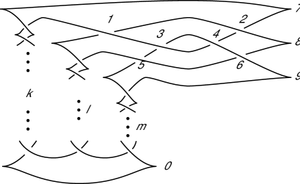
$a_{1}$$a_{2}$$b_{1}$$b_{2}$$c_{1}$$c_{2}$$t_{1}$$t_{2}$$t_{3}$$t_{0}$$k$$l$$m$

Figure 3. This knot is distinguished from its Legendrian mirror by its cohomology ring. The crossings along the left most, center and right most legs are denoted, respectively, by $x_{i},$ $y_{i},$ and $z_{i}.$ Similarly the crossings coming from resolving the right cusps along these legs are denoted by $t^{x}_{i},t^{y}_{i}$ and $t^{z}_{i}$ respectively.

Proof of the first part of Theorem 1.1.

For infinitely many choices of $k,l,m$, the Legendrian knot in Figure 3 is not Legendrian isotopic to its Legendrian mirror. The knot and its mirror have the same classical invariants and the same linearized cohomology, but different linearized cohomology rings.

To see this, we first compute the gradings of the generators:

$$|a_{1}|=-|a_{2}| =k-l-1$$

$$|b_{1}|=-|b_{2}| =k-m-1$$

$$|c_{1}|=-|c_{2}| =l-m-1$$

$$|t_{i}|=|t^{x}_{i}|=|t^{y}_{i}|=|t^{z}_{i}| =1$$

$$|x_{i}|=|y_{i}|=|z_{i}| =0$$

For infinitely many choices of $k,l,m$, the gradings in each row will be distinct.

The differential has the following form:

$$\partial a_{1} =0 \partial t_{1} =1+x_{1}(1+a_{1}a_{2}+b_{1}b_{2})$$

$$\partial a_{2} =y_{1}c_{1}b_{2} \partial t_{2} =1+(1+a_{2}a_{1})y_{1}(1+c_{1}c_{2})$$

$$\partial t_{3} =1+(1+b_{2}b_{1}+c_{2}c_{1})z_{1}$$

$$\partial b_{1} =a_{1}y_{1}c_{1} \partial t_{0} =1+x_{k+1}y_{l+1}z_{m+1}$$

$$\partial b_{2} =0$$

$$\partial t^{x}_{i} =1+x_{i}x_{i+1}$$

$$\partial c_{1} =0 \partial t^{y}_{i} =1+y_{i}y_{i+1}$$

$$\partial c_{2} =b_{2}a_{1}y_{1} \partial t^{z}_{i} =1+z_{i}z_{i+1}$$

Recall that for the Legendrian mirror of $K$, the ordering of the generators in the differential are all reversed. In either case, since all but at most one of the $a_{i}$, $b_{i}$, or $c_{i}$ have nonzero grading, then there is a unique augmentation $\varepsilon$ that sends the $x_{i}$, $y_{i}$, and $z_{i}$ to $1$ and all other generators to $0$.

The linearized codifferential $\delta^{\varepsilon}$ of all generators $a_{i}$, $b_{i}$, and $c_{i}$ vanishes (where we again abuse notation and identify a generator with its dual), as does the linearized codifferential of the generators coming from the right cusps. The linearized codifferentials of the $x_{i}$, $y_{i}$, and $z_{i}$ generators are sums of “adjacent” right cusp generators, so they show that the generators coming from the right cusps are all equal in cohomology. Thus, we have the following compuation:

(4.1) $$LCH^{k}_{\varepsilon}(K)=\langle[a_{i}],[b_{i}],[c_{i}],[t]\rangle.$$

The nontrivial cup products are:

$$[a_{1}]\cup[a_{2}]=[a_{2}]\cup[a_{1}] =[t] [c_{1}]\cup[b_{2}] =[a_{2}]$$

$$[b_{1}]\cup[b_{2}]=[b_{2}]\cup[b_{1}] =[t] [a_{1}]\cup[c_{1}] =[b_{1}]$$

$$[c_{1}]\cup[c_{2}]=[c_{2}]\cup[c_{1}] =[t] [b_{2}]\cup[a_{1}] =[c_{2}]$$

The cup products in the left column will be interpreted as part of a Poincaré duality pairing in the next section. The cup products in the right column are not symmetric; the first, for example, is a nontrivial map from $LCH^{l-m-1}_{\varepsilon}\otimes LCH^{m-k+1}_{\varepsilon}\to LCH^{l-k+1}_{\varepsilon}$. Under the assumption that the generators $a_{i}$, $b_{i}$, and $c_{i}$ have distinct gradings, we can then easily see that no such nontrivial cup product exists in the cohomology ring of the Legendrian mirror. Hence, the knot $K$ and its Legendrian mirror are not Legendrian isotopic. ∎

Remark 4.3.

There are examples of Legendrian knots with small crossing number that have augmentations with noncommutative linearized cohomology rings: consider, for example, the mirrors of the knots $8_{21}$, $9_{45}$, or $9_{47}$ in Melvin and Shrestha’s table [19].

4.2. Duality

We are now ready to prove Theorem 1.3 concerning the duality in [27]. We note that Theorem 1.3 implies the product operation in the ring structure of linearized contact cohomology is non-trivial, while the first part of Theorem 1.1 shows that there are non-trivial products that are not forced by the duality theorem.

Proof of Theorem 1.3.

As described in [27], there is chain complex $(Q_{*},\partial_{Q})$ that can be thought of in two ways: first, it is the mapping cone for a map $\rho:(A_{*},\partial^{\varepsilon}_{1})\to CM_{*}(S^{1};f)$, where $CM_{*}$ is the Morse complex for a Morse function $f$ on $S^{1}$. As noted in [5], the long exact sequence of the mapping cone is:

(4.2) $$\cdots\to H_{k+1}(S^{1})\to H_{k}(Q)\to LCH^{\varepsilon}_{k}(K)\stackrel{{\scriptstyle\rho_{*}}}{{\to}}H_{k}(S^{1})\to\cdots.$$

Further, $\rho_{*}$ is trivial in dimension $0$ and onto in dimension $1$; see the discussion after Lemma 4.9 of [27] or Theorem 5.5 of [5].

The second perspective on $H_{*}(Q)$ is that there exists an isomorphism $\eta_{*}:H_{k}(Q)\to LCH^{-k}_{\varepsilon}(K)$. Putting these viewpoints together yields the isomorphisms:

$$LCH^{1}_{\varepsilon}(K) \simeq LCH_{-1}^{\varepsilon}(K)\oplus H_{0}(S^{1})$$

$$LCH_{1}^{\varepsilon}(K) \simeq LCH^{-1}_{\varepsilon}(K)\oplus H_{1}(S^{1})$$

$$LCH^{k}_{\varepsilon}(K) \simeq LCH_{-k}^{\varepsilon}(K) k\neq\pm 1.$$

Let $c$ be the image under $\eta_{*}$ of a generator of $H_{0}(S^{1})$ and define:

(4.3) $$\overline{LCH}_{\varepsilon}^{1}=\eta_{*}LCH_{-1}^{\varepsilon}(K).$$

Finally, we define $\kappa\in LCH_{1}^{\varepsilon}(K)$ to come from $H_{1}(S^{1})$. The main theorem of [5] shows that $\kappa$ is the unique class that pairs to $1$ with $c$ and pairs to $0$ on $\overline{LCH}_{\varepsilon}^{1}$, and hence agrees with the $\kappa$ defined in Theorem 5.1 of [27].

The map $\eta_{*}$ has an inverse $\phi_{*}$ which comes from a “cap product”. More specifically, the chain map $\phi(p)$ is constructed in [27] by counting immersed disks with one negative corner at $p$, one negative corner at the output $q^{\prime}$, one positive corner at $r$ with $\langle r,\kappa\rangle=1$ (in that counterclockwise order), and possibly other negative augmented corners. Such disks, however, also contribute to the evaluation of the product $m_{2}(p,p^{\prime})$ on $\kappa$. Passing to homology, we obtain:

(4.4) $$\langle[p^{\prime}],\phi_{*}[p]\rangle=\langle[p]\cup[p^{\prime}],\kappa\rangle.$$

Since $\phi_{*}$ is invertible on $\overline{LCH}^{*}_{\varepsilon}$, the pairing on the right must be nondegenerate, as desired.

To see that the pairing is symmetric, notice that we could have defined a map $\hat{\phi}$ using disks with one negative corner at $p$, one positive corner at $r$ with $\langle r,\kappa\rangle=1$, one negative corner at the output $q^{\prime}$ (in that counterclockwise order), and possibly other negative augmented corners. The induced map $\hat{\phi}_{*}$ also serves as an inverse for $\eta_{*}$, and hence must be the same map as $\phi_{*}$. Thus:

$$\langle[p]\cup[p^{\prime}],\kappa\rangle =\langle[p^{\prime}],\phi_{*}[p]\rangle$$

$$=\langle[p^{\prime}],\hat{\phi}_{*}[p]\rangle$$

$$=\langle[p^{\prime}]\cup[p],\kappa\rangle.$$

∎

4.3. The Massey Product

In this subsection, we study the Massey product on the linearized contact cohomology of a Legendrian knot in more detail. Using the same notation as in Section 4.1, we summarize the discussion of the product from the Subsection 3.1 in the following corollary:

Corollary 4.4.

If $[a],[b]$ and $[c]$ are elements in $LCH^{*}_{\varepsilon}(K)$ of degrees $r,s$ and $t,$ respectively such that

$$[a]\cup[b]=0=[b]\cup[c]$$

then there is a well defined element

$$\{[a],[b],[c]\}\in\frac{LCH^{r+s+t+1}_{\varepsilon}(K)}{\bigl{(}\operatorname{Im}(\mu^{\varepsilon}_{2}([a],\cdot))+\operatorname{Im}(\mu^{\varepsilon}_{2}(\cdot,[c]))\bigr{)}\cap LCH^{r+s+t+1}_{\varepsilon}(K)}$$

given by

$$[m^{\varepsilon}_{3}(a,b,c)+m^{\varepsilon}_{2}(a,y)+m^{\varepsilon}_{2}(x,c)],$$

where $\delta^{\varepsilon}x=m^{\varepsilon}_{2}(a,b)$ and $\delta^{\varepsilon}y=m^{\varepsilon}_{2}(b,c)$.

Example 4.5.

Consider the Legendrian trefoil $K$ from Figure 2 again. We computed the $A_{\infty}$-algebra structure in Example 3.4 and the product structure in Example 4.2. Even though $m_{3}^{\varepsilon}\not=0$, one may easily check that all Massey products are trivial in this example.

Notice that if one wants to compare the Massey product structures on the linearized contact cohomologies of two Legendrian knots one must first have an isomorphism of their cohomology rings (that is, an isomorphism that preserves the product structure). The Massey product can be non-trivial and distinguish Legendrian knots that are not distinguished by their linearized contact cohomology ring structures.

Proof of second part of Theorem 1.1.

The Legendrian knot $K$ in Figure 4 is not isotopic to its Legendrian mirror. The two knots can be distinguished using the Massey products on the linearized contact cohomology but not by their linearized contact cohomology rings.

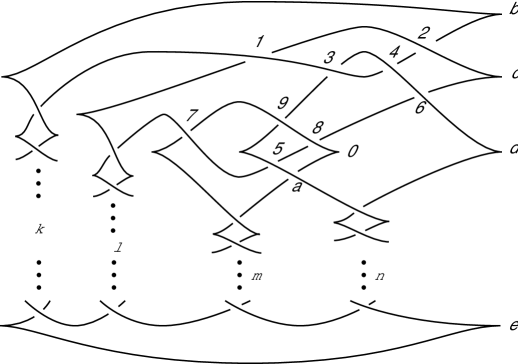
$a_{1}$$a_{2}$$b_{1}$$b_{2}$$e_{1}$$e_{0}$$c_{0}$$f$$c_{1}$$s_{4}$$d$$t_{1}$$t_{2}$$t_{3}$$t_{0}$$k$$l$$m$$n$

Figure 4. This knot is distinguished from its Legendrian mirror by its Massey products. The crossings along the left most, center left, center right and right most legs are denoted, respectively, by $x_{i},$ $y_{i},z_{i}$ and $w_{i}.$ Similarly the right cusps along these legs are denoted by $t^{x}_{i},t^{y}_{i},t^{z}_{i}$ and $t^{w}_{i}$ respectively.

To see this, we first compute the gradings of the generators:

$$|a_{1}|=-|a_{2}|=k-l-1 |b_{1}|=-|b_{2}|=k-n-1$$

$$|c_{1}|=-|d|=m-n |c_{0}|=-|f|=l-m-1$$

$$|e_{0}|=|e_{1}|+1=l-n-1 |t_{i}|=|t^{x}_{i}|=|t^{y}_{i}|=|t^{z}_{i}|=|t^{w}_{i}|=1$$

$$|x_{i}|=|y_{i}|=|z_{i}|=|w_{i}|=0$$

For infinitely many choices of $k,l,m$, and $n$, the gradings in each row and column will be distinct.

The differential has the following form:

$$\partial a_{1} =0 \partial t_{1} =1+x_{1}(1+a_{1}a_{2}+b_{1}b_{2})$$

$$\partial a_{2} =y_{1}c_{0}c_{1}b_{2} \partial t_{2} =1+(1+a_{2}a_{1})y_{1}(1+c_{0}f+c_{0}c_{1}e_{0})+a_{2}b_{1}e_{1}$$

$$\partial t_{3} =1+[1+b_{2}b_{1}+(1+b_{2}b_{1})dc_{1}]w_{1}$$

$$\partial b_{1} =a_{1}y_{1}c_{0}c_{1} \partial t_{4} =1+(1+fc_{0})z_{1}+c_{1}d$$

$$\partial b_{2} =0 \partial t_{0} =1+x_{k+1}y_{l+1}z_{m+1}w_{n+1}$$

$$\partial c_{0} =\partial c_{1}=0 \partial t^{x}_{i} =1+x_{i}x_{i+1}\text{ and similarly for }t^{y}_{i},t^{z}_{i},t^{w}_{i}$$

$$\partial d =e_{1}c_{0} \partial e_{0} =(1+b_{2}b_{1})e_{1}$$

$$\partial f =c_{1}e_{1} \partial e_{1} =0$$

Since we assume that only the $x_{i}$, $y_{i}$, $z_{i}$, and $w_{i}$ have zero grading, there is a unique augmentation that sends these generators to $1$ and all others to $0$. Abusing notation to identify generators and their duals, we see that the linearized cohomology is given by:

(4.5) $$LCH^{k}_{\varepsilon}(K)=\langle[a_{i}],[b_{i}],[c_{i}],[d],[f],[t]\rangle,$$

where $[t]$ is once again any one of the right cusps.

Duality pairs the $[a_{i}]$, the $[b_{i}]$, $[c_{0}]$ with $[f]$, and $[c_{1}]$ with $[d]$. There are no other nontrivial cup products; in fact, all cup products between cocycles (beyond those involved in the duality pairing) vanish at the cochain level. Thus, it follows that the $m_{3}$ products between triples of cocycles yield two Massey products:

$$\{[c_{0}],[c_{1}],[b_{2}]\} =[a_{2}],$$

$$\{[a_{1}],[c_{0}],[c_{1}]\} =[b_{1}].$$

Since the only class in the image of the cup product is $[t]$, the Massey products above lie in $\overline{LCH}^{*}_{\varepsilon}(K)$, and hence are nontrivial. Under the assumption that the generators $a_{i}$, $b_{i}$, and $c_{i}$ have distinct gradings, we can then easily see that there are no nontrivial Massey products in these gradings in the linearized cohomology of the Legendrian mirror. Hence, the knot $K$ and its Legendrian mirror are not Legendrian isotopic even though their linearized cohomology rings are isomorphic. ∎

4.4. Higher-Order Massey Products

As in the previous subsections, we can show that the higher-order Massey products are also nontrivial.

Completion of the Proof of Theorem 1.1.

The Legendrian knot $K_{n}$ in Figure 5 is not isotopic to its Legendrian mirror. The two knots can be distinguished using the $(n+1)^{\text{st}}$-order Massey products on the linearized contact cohomology but not by their linearized contact cohomology rings or their $m^{\text{th}}$-order Massey products for $m\leq n$.

By a similar calculation to the previous examples, one can show that the cup products (besides those associated with duality) and the lower-order Massey products all vanish, so the $(n+1)^{\text{st}}$-order Massey product lies in $\overline{LCH}^{*}_{\varepsilon}(K)$. Further, the cup product and lower-order Massey products vanish at the chain level, so we have the following two Massey products whose gradings are nonsymmetric:

$$\{[c_{0}],\ldots,[c_{n}],[b_{2}]\} =[a_{2}]$$

$$\{[a_{1}],[c_{0}],\ldots,[c_{n}]\} =[b_{1}].$$

It follows that the knot $K_{n}$ is not isotopic to its Legendrian mirror. ∎

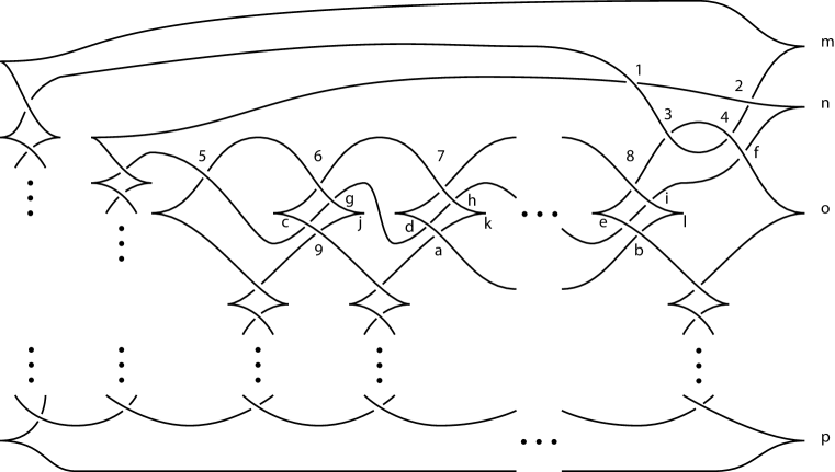
$a_{1}$$a_{2}$$b_{1}$$b_{2}$$c_{0}$$c_{1}$$c_{2}$$c_{m}$$d_{1}$$d_{2}$$d_{m}$$e_{1}$$e_{2}$$e_{m}$$e_{0}$$f_{1}$$f_{2}$$f_{m}$$t_{1}$$t_{2}$$t_{m}$$s_{1}$$s_{2}$$s_{3}$$s_{0}$

Figure 5. This knot is distinguished from its Legendrian mirror by its order $n+1$ Massey products.

Remark 4.6.

Using the “splashes” of [11] or the “dips” of [26], it is possible to show that the $A_{\infty}$ structure on the linearized cochain complex is $A_{\infty}$ quasi-isomorphic to one for which $m_{k}=0$ for all $k\geq 4$. As the examples above show, however, this does not mean that the $A_{\infty}$ structure $\boldsymbol{\mu}$ on the linearized contact cohomology is trivial for $k\geq 4$.

5. Products and Higher Order Linearizations

In this section, we explore the relationship between the $A_{\infty}$ structure on the linearized contact cohomology, associated product structures, and Chekonov’s order $n$ linearizations.

5.1. The Minimal Model Theorem, Revisited

We begin by sketching the proof of the Minimal Model Theorem 3.2 following Markl’s formulae in [18]; see also [15, 16, 20, 28]. First, let us describe the construction of the maps of $\boldsymbol{\mu}$. The fact that we are working over the field $\mathbb{Z}_{2}$ allows us to choose maps $i:H^{*}(V)\to V$, $p:V\to H^{*}(V)$, and $h:V\to V$ such that:

(5.1) $$p\circ i=\operatorname{Id}\quad\text{and}\quad\operatorname{Id}+i\circ p=\delta h+h\delta.$$

We next consider the set $\Gamma_{k}$ of rooted planar trees with $k$ leaves (the root edge is not counted among the $k$ leaves) and at least trivalent internal vertices. For each $T\in\Gamma_{k}$, we construct a map $g_{T}:V^{\otimes k}\to V$ by placing the inputs in order along the $k$ leaves, an $m_{k}$ at each $(k+1)$-valent internal vertex, and an $h$ at each internal edge; see Figure 6. The map $g_{T}$ is then defined by appropriately inserting arguments and composing maps from the leaves down to the root. We then define $g_{1}=\delta$ and for $k\geq 2$, the maps:

$$g_{k}=\sum_{T\in\Gamma_{k}}g_{T}.$$

These maps form a sequence $\mathbf{g}$.

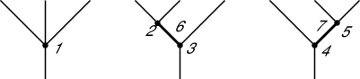
$m_{3}$$m_{2}$$m_{2}$$m_{2}$$m_{2}$$h$$h$

Figure 6. The rooted trees that make up the map $g_{3}$. The rightmost tree gives the map $g_{T}(a,b,c)=m_{2}(a,h\circ m_{2}(b,c))$.

The products $\boldsymbol{\mu}$ are then defined by:

$$\mu_{k}=p\circ g_{k}\circ(i\otimes\cdots\otimes i).$$

The product $\mu_{3}:H^{*}(V)^{\otimes 3}\to H^{*}(V)$, for example, is defined as follows, where we write $i(\alpha_{k})=a_{k}$:

$$\mu_{3}(\alpha_{1},\alpha_{2},\alpha_{3})= \,\,p\bigl{(}m_{3}(a_{1},a_{2},a_{3})$$

$$+m_{2}\left(a_{1},h\circ m_{2}(a_{2},a_{3})\right)+m_{2}\left(h\circ m_{2}(a_{1},a_{2}),a_{3}\right)\bigr{)}.$$

The maps $i$, $p$, and $h$ can also be extended to sequences of maps $\mathbf{i}$, $\mathbf{p}$, and $\mathbf{h}$. The map $i_{k}$, for example, is defined by $i_{k}=h\circ g_{k}\circ(i\otimes\cdots\otimes i)$. The formulae for $p_{k}$ and $h_{k}$ are also based on rooted planar trees, but are somewhat more involved.

Proposition 5.1 (Markl [18]).

The maps $\boldsymbol{\mu}$ give an $A_{\infty}$ structure on $H^{*}(V)$, the maps $\mathbf{i}$ and $\mathbf{p}$ are $A_{\infty}$ morphisms, and the maps $\mathbf{h}$ are an $A_{\infty}$ homotopy between $\mathbf{i}\circ\mathbf{p}$ and the identity on $V$.

Here, an $A_{\infty}$ homotopy between two $A_{\infty}$ morphisms $f,g:(V,\mathbf{m})\to(W,\mathbf{n})$ is a sequence of degree $-1$ maps $h_{n}:V^{\otimes n}\to V$ that satisfy:

$$f_{n}+g_{n}=\sum_{i+j+k=n}h_{i+1+k}\circ(1^{\otimes i}\otimes m_{j}\otimes 1^{\otimes k})+\sum_{\begin{subarray}{c}1\leq k\leq r\leq n\\ i_{1}+\ldots+i_{r}=n\end{subarray}}n_{r}\circ(f_{i_{1}}\otimes\cdots\otimes f_{i_{k-1}}\otimes h_{i_{k}}\otimes g_{i_{k+1}}\otimes\cdots\otimes g_{i_{r}}).$$

Remark 5.2.

In particular, we have that $\mathbf{i}$ is the $A_{\infty}$ quasi-isomorphism promised by the Minimal Model Theorem. Note that the proposition also yields $A_{n}$ morphisms and homotopies by stopping the construction at any finite step.

5.2. $A_{\infty}$ Structures Determine Massey Products

The relationship between the $A_{\infty}$ structure on $H^{*}(V)$ and the Massey products is straightforward to state:

Proposition 5.3 (Kadeishvili [14]).

Given $\alpha_{k}\in H^{*}(V)$, $k=1,2,3$, such that

$$\mu_{2}(\alpha_{1},\alpha_{2})=0=\mu_{2}(\alpha_{2},\alpha_{3}),$$

the projection of $\mu_{3}(\alpha_{1},\alpha_{2},\alpha_{3})$ to $\tilde{H}^{*}(V)$ agrees with the Massey product $\{\alpha_{1},\alpha_{2},\alpha_{3}\}$.

To see this, choose $x=h\circ m_{2}(a_{1},a_{2})$ and $y=h\circ m_{2}(a_{2},a_{3})$. Notice that:

$$\delta x =m_{2}(a_{1},a_{2})+i\circ p\circ m_{2}(a_{1},a_{2})+h\delta m_{2}(a_{1},a_{2})$$

$$=m_{2}(a_{1},a_{2}).$$

Note that the last term in the first line vanishes since $m_{2}(a_{1},a_{2})$ is a cycle, and the second-to-last term vanishes since $m_{2}(a_{1},a_{2})$ represents the zero cohomology class by assumption. A similar fact holds for $y$, so we may take $x$ and $y$ to be the elements required for the definition of the Massey product $\{\alpha_{1},\alpha_{2},\alpha_{3}\}$. Now we need only compute that:

$$\mu_{3}(\alpha_{1},\alpha_{2},\alpha_{3}) =p\bigl{(}m_{3}(a_{1},a_{2},a_{3})+m_{2}\left(a_{1},h\circ m_{2}(a_{2},a_{3})\right)$$

$$\quad+m_{2}\left(h\circ m_{2}(a_{1},a_{2}),a_{3}\right)\bigr{)}$$

$$=p(m_{3}(a_{1},a_{2},a_{3})+m_{2}(a_{1},y)+m_{2}(x,a_{3})),$$

which, by definition, projects to the Massey product.

In fact, this is the base case for a proof of a similar statement for order $n$ Massey products defined using the full $A_{n}$ structure. The proof of this folk theorem is a straightforward generalization of that in [17] using the language introduced above.

5.3. $A_{\infty}$ Structure on $LCH_{\epsilon}^{*}$ and Higher Order Linearizations.

We are finally ready to prove Theorem 1.2, which states that the $A_{n}$ structure on $LCH^{*}_{\varepsilon}$ is strictly stronger than the $n^{\text{th}}$-order linearized cohomology. Before proving the theorem, however, we need to introduce one more algebraic object, Stasheff’s tilde construction $(\tilde{B}^{n}(V),d^{n})$ of an $A_{n}$ algebra $(V,\mathbf{m})$ [29]. The chains of this complex lie in

$$\tilde{B}^{n}(V)=\bigoplus_{k=1}^{n}V^{\otimes k},$$

while the differential $d^{n}$ is defined componentwise by:

(5.2) $$d^{n}|_{V^{\otimes a}}=\sum_{i+j+k=a}1^{\otimes i}\otimes m_{j}\otimes 1^{\otimes k}.$$

That this differential satisfies $(d^{n})^{2}=0$ follows from the defining $A_{\infty}$ equation (3.1). The reason that we introduce the tilde construction is the following result.

Lemma 5.4.

The $n^{\text{th}}$-order linearized cochain complex with respect to $\varepsilon$ is the tilde construction of $(A^{*},\mathbf{m}^{\varepsilon})$.

Proof.

Clearly, we have that $A_{(n)}=\bigoplus_{i=1}^{n}A^{\otimes i}$ and the differential $\partial^{\varepsilon}_{(n)}$ is equivalent to the following, essentially because of the Leibniz rule and the fact that any term of length greater than $n$ becomes zero in $A_{(n)}$:

$$\partial^{\varepsilon}_{(n)}|=\sum_{i+j+k\leq n}1^{\otimes i}\otimes\partial^{\varepsilon}_{j}\otimes 1^{\otimes k}.$$

Dually, it is now easy to see that the $n^{\text{th}}$-order linearized cochain complex has cochains in $\bigoplus_{i=1}^{n}(A^{*})^{\otimes i}$ and codifferential $\delta^{\varepsilon}_{(n)}$ defined precisely as in Equation (5.2). ∎

It is straightforward to see that $A_{n}$ morphisms and homotopies translate to similar notions for the tilde construction (see, for example, [18, 28]).

Lemma 5.5.

1. An $A_{n}$ morphism $f:(V,\mathbf{m})\to(W,\mathbf{n})$ determines a chain map $\tilde{B}^{n}f:\tilde{B}^{n}V\to\tilde{B}^{n}W$ whose $V^{\otimes a}$ component is

   $$\sum_{r}\sum_{i_{1}+\cdots+i_{r}=a}f_{i_{1}}\otimes\cdots\otimes f_{i_{r}}.$$

2. An $A_{n}$ homotopy $h:(V,\mathbf{m})\to(W,\mathbf{n})$ between $f$ and $g$ determines a chain homotopy $\tilde{B}^{n}h:\tilde{B}^{n}V\to\tilde{B}^{n}W$ between $\tilde{B}^{n}f$ and $\tilde{B}^{n}g$.

We are now ready to prove Theorem 1.2.

Proof of Theorem 1.2.

We begin by proving that the $A_{n}$ structure on the linearized cohomology determines the $n^{\text{th}}$-order linearized cohomology. Fix an augmentation $\varepsilon$. By the remarks in Section 5.1, we know that the $A_{n}$ structures on the linearized cochain complex $(A^{*},\delta^{\varepsilon})$ and the linearized cohomology $LCH^{*}_{\varepsilon}$ are $A_{\infty}$ homotopy equivalent. The lemma above then implies that their tilde constructions are chain homotopy equivalent, and hence have isomorphic cohomologies. Since the $A_{n}$ structure on $LCH^{*}_{\varepsilon}$ determines the cohomology of its tilde construction, it also determines the cohomology of the tilde construction of the $A_{n}$ structure on $A^{*}$ which, by Lemma 5.4, is simply $LCH^{*}_{\varepsilon}(K,n)$. This proves the first half of the theorem.

To prove that the $A_{n}$ structure is strictly stronger, we observe that since order $n$ Massey products be used to distinguish the Legendrian knots in Theorem 1.1 from their Legendrian mirrors, Proposition 5.3 and its order $n$ generalization implies that the $A_{n}$ structures also distinguish these knots. On the other hand, the higher-order cohomologies can never distinguish a Legendrian knot $K$ from its Legendrian mirror $\overline{K}$. To see why, notice that the reflection map $\tau:A_{(n)}\to A_{(n)}$ defined by:

$$\tau(a_{1}\otimes\cdots\otimes a_{n})=a_{n}\otimes\cdots\otimes a_{1}$$

gives a quasi-isomorphism (but not necessarily a tame isomorphism) between $(A_{(n)},\partial_{(n)})$ and $(\overline{A}_{(n)},\overline{\partial}_{(n)})$. ∎

5.4. An Alternative Proof when $n=2$

In this final section, we present a more down-to-earth proof that, for a fixed augmentation, the linearized cohomology ring is strictly stronger than the order $2$ linearized cohomology, i.e. the $n=2$ case of Theorem 1.2.

First, write $A_{(2)}$ as $A\oplus A^{\otimes 2}$. For ease of exposition, we drop the augmentation $\epsilon$ from the notation. In this notation, the codifferential can be recorded by:

(5.3) $$\delta_{(2)}=\begin{bmatrix}\delta&m_{2}\\ 0&\delta^{\otimes}\end{bmatrix},$$

which implies the following lemma:

Lemma 5.6.

The second order linearized cochain complex is the mapping cone of the degree $1$ chain map $m_{2}:((A^{*})^{\otimes 2},\delta^{\otimes})\to(A^{*},\delta)$.

Associated to this mapping cone we have the standard long exact sequence:

$$\cdots\to LCH^{k}(K)\to LCH^{k}(K,2)\to H^{k}((A^{*})^{\otimes 2},\delta^{\otimes})\stackrel{{\scriptstyle d^{*}}}{{\to}}LCH^{k+1}(K)\to\cdots.$$

Since we are working over a field, the Künneth formula gives us:

$$H^{k}((A^{*})^{\otimes 2},\delta^{\otimes})=\bigoplus_{i+j=k}LCH^{i}\otimes LCH^{j}.$$

Moreover, we know that the connecting homomorphism $d^{*}$ is induced by $m_{2}.$ That is, it is given by the cup product $\mu_{2}$. Again, since we are working over a field, the short exact sequences into which the long exact sequence above decomposes must all split. This gives:

(5.4) $$LCH^{k}(K,2)\simeq\ker\mu_{2}\oplus\bigl{(}LCH^{k}(K)/\operatorname{Im}\mu_{2}\bigr{)}.$$

In other words, the second-order linearization is determined by the image and kernel of the cup product map on linearized contact cohomology. Thus, the linearized cohomology and the cup product determine the second-order linearized cohomology.

References

- [1] D. Bennequin, Entrelacements et equations de Pfaff, Asterisque 107–108 (1983), 87–161.
- [2] Yu. Chekanov, Differential algebra of Legendrian links, Invent. Math. 150 (2002), 441–483.
- [3] Yu. Chekanov and P. Pushkar, Combinatorics of Legendrian links and the Arnol’d -conjectures, Russ. Math. Surv. 60 (2005), no. 1, 95–149.
- [4] F. Ding and H. Geiges, Legendrian knots and links classified by classical invariants, Commun. Contemp. Math. 9 (2007), no. 2, 135–162.
- [5] T. Ekholm, J. Etnyre, and J. Sabloff, A duality exact sequence for Legendrian contact homology, Preprint available as arXiv:0803.2455, 2008.
- [6] Ya. Eliashberg, Invariants in contact topology, Proceedings of the International Congress of Mathematicians, Vol. II (Berlin, 1998), no. Extra Vol. II, 1998, pp. 327–338 (electronic).
- [7] Ya. Eliashberg and M. Fraser, Classification of topologically trivial Legendrian knots, Geometry, topology, and dynamics (Montreal, PQ, 1995), Amer. Math. Soc., Providence, RI, 1998, pp. 17–51.
- [8] J. Etnyre, Legendrian and transversal knots, Handbook of knot theory, Elsevier B. V., Amsterdam, 2005, pp. 105–185.
- [9] J. Etnyre and K. Honda, Knots and contact geometry I: Torus knots and the figure eight knot, J. Symplectic Geom. 1 (2001), no. 1, 63–120.
- [10] J. Etnyre, L. Ng, and J. Sabloff, Invariants of Legendrian knots and coherent orientations, J. Symplectic Geom. 1 (2002), no. 2, 321–367.
- [11] D. Fuchs, Chekanov-Eliashberg invariant of Legendrian knots: existence of augmentations, J. Geom. Phys. 47 (2003), no. 1, 43–65.
- [12] D. Fuchs and T. Ishkhanov, Invariants of Legendrian knots and decompositions of front diagrams, Mosc. Math. J. 4 (2004), no. 3, 707–717.
- [13] D. Fuchs and S. Tabachnikov, Invariants of Legendrian and transverse knots in the standard contact space, Topology 36 (1997), 1025–1053.
- [14] T. Kadeišvili, On the theory of homology of fiber spaces, Uspekhi Mat. Nauk 35 (1980), no. 3(213), 183–188, International Topology Conference (Moscow State Univ., Moscow, 1979).
- [15] H. Kajiura, Noncommutative homotopy algebras associated with open strings, Rev. Math. Phys. 19 (2007), no. 1, 1–99.
- [16] M. Kontsevich and Y. Soibelman, Homological mirror symmetry and torus fibrations, Symplectic geometry and mirror symmetry (Seoul, 2000), World Sci. Publ., River Edge, NJ, 2001, pp. 203–263.
- [17] D.-M. Lu, J. Palmieri, Q.-S. Wu, and J. Zhang, A-infinity structure on Ext-algebras, Preprint, 2007.
- [18] M. Markl, Transferring (strongly homotopy associative) structures, Rend. Circ. Mat. Palermo (2) Suppl. (2006), no. 79, 139–151.
- [19] P. Melvin and S. Shrestha, The nonuniqueness of Chekanov polynomials of Legendrian knots, Geom. Topol. 9 (2005), 1221–1252.
- [20] S. A. Merkulov, Strong homotopy algebras of a Kähler manifold, Internat. Math. Res. Notices (1999), no. 3, 153–164.
- [21] L. Ng, Computable Legendrian invariants, Topology 42 (2003), no. 1, 55–82.
- [22] L. Ng and J. Sabloff, The correspondence between augmentations and rulings for Legendrian knots, Pacific J. Math. 224 (2006), no. 1, 141–150.
- [23] P. Ozsváth, Z. Szabó, and D. Thurston, Legendrian knots, transverse knots and combinatorial Floer homology, Geom. Topol. 12 (2008), no. 2, 941–980.
- [24] D. Rutherford, Thurston-Bennequin number, Kauffman polynomial, and ruling invariants of a Legendrian link: the Fuchs conjecture and beyond, Int. Math. Res. Not. (2006), Art. ID 78591, 15.
- [25] J. Sabloff, Invariants for Legendrian knots from contact homology, In preparation.
- [26] by same author, Augmentations and rulings of Legendrian knots, Int. Math. Res. Not. (2005), no. 19, 1157–1180.
- [27] by same author, Duality for Legendrian contact homology, Geom. Topol. 10 (2006), 2351–2381 (electronic).
- [28] V. Smirnov, Simplicial and operad methods in algebraic topology, Translations of Mathematical Monographs, vol. 198, American Mathematical Society, Providence, RI, 2001, Translated from the Russian manuscript by G. L. Rybnikov.
- [29] J. Stasheff, Homotopy associativity of -spaces. ii, Trans. Amer. Math. Soc. 108 (1963), no. 2, 293–312.