Comments on QED with background electric fields

Abstract

It is well known that there is a total cancellation of the factorizable IR divergences in unitary interacting field theories, such as QED and quantum gravity. In this note we show that such a cancellation does not happen in QED with background electric fields which can produce pairs. There is no factorization of the IR divergences.

1 Introduction

The particle creation in external fields is among the most interesting problems in quantum field theory. The effect of pair creation in QED with external electric field was investigated from different points of view in many places. The pair creation rate was calculated in [1].

There are two reasons why we would like to address QED in electric field background. The first one is that we would like to define an appropriate setting to take into account the back-reaction of the pair production on to the external field. The second reason of considering the QED with background electric field is its similarity with QFT on curved de Sitter background, which goes beyond [2] the pair creation [3],[4] and acceleration of particles.

In particular, here we are interested in the IR behavior of QED with electric field background. It is well known that there is total cancellation of IR divergences in QED without background fields [5]. The latter consideration can be linked to the fact that mass-shell electrons can not radiate mass–shell photons. In fact, consider the process $e^{-}\rightarrow\gamma+e^{-*}$. Obviously the amplitude of this process in the leading order is proportional to:

$$A\propto\langle 0,\mbox{out}|a_{k}^{-}\beta_{q}^{-}\int dt\,\hat{H}_{int}(t)\,a_{p}^{+}|0,\mbox{in}\rangle\propto\int{d^{4}x}e^{i(p-q-k)x}\propto\delta^{(4)}\left(p-q-k\right),$$

i.e. obviously there is the energy-momentum conservation at the vertex in QED, if there are no any background fields: $p=k+q$, where $p,q,k$ – are momenta of the incoming electron and outgoing photon and electron, respectively; $\hat{H}_{int}$ – is the QED interaction Hamiltonian describing the interactions between electrons and photons. All of the three legs of the amplitude are on-shell. Hence, $k^{2}-m^{2}=p^{2}-m^{2}=0$ and $q^{2}=0$. Due to the latter relations the argument of the $\delta$-function is never zero. Hence, the amplitude is zero, which just means that there is no radiation on mass-shell.

However, if one of the particles is off-shell, say $k^{2}-m^{2}=\lambda$, where $\lambda$ is the virtuality, then for the amplitude to be non-vanishing it has to be that $\lambda=-2pq$. Such a dependence of $\lambda$ on $q$ is important for the factorization of IR divergences, which, in turn, is important for their cancellation to all orders [5], [6]. Note that such a relation between the virtuality of the matter field and the momentum of the radiated particle is a very special situation following from the energy–momentum four–vector conservation at the vertices and from the standard dispersion relations.

Let us sketch here the physical meaning of the cancellation of the IR divergences. One can immediately notice that loop corrections to any processes in QED have IR divergences, which are all of the same order (independently of the number of loops) as the IR cut-off parameter is taken to zero [5], [6]. E.g. the first loop corrections have a characteristic IR divergence as follows:

$$\mbox{IR}_{\mbox{\scriptsize{loop}}}\propto\int\frac{d^{4}q}{(pq)^{2}q^{2}}\propto\log{m_{0}}$$

with the cut-off $m_{0}\rightarrow 0$. Due to the factorization of the IR divergences higher loops bring just powers of such an expression [5]. Because of such contributions, if the IR cut-off is taken to zero, all the cross–sections in QED appear to be zero, which is quite puzzling.

The resolution of this problem comes with the understanding that any scattering process of hard particles is accompanied with the emission of the tree level soft photons (because electrons do accelerate during the scattering process) [5]. As the result the cross–sections of hard processes are dressed with the powers (due to the factorization) of the contribution as follows. The amplitude for the emission of a soft photon (with the momentum $|\vec{q}|\to 0$) is proportional to the propagator of the virtual particle, which, in its own right, is proportional to its inverse virtuality $1/\lambda\propto 1/(pq)$. The latter behavior of the propagator follows from the presence of the above mentioned $\delta$–function (enforcing energy conservation) in the interaction vertex.

Thus, after the integration over the invariant phase volume of the emitted photon, the factor contributing to the cross-section is proportional to [5]:

$$\int|M(k,q;p)|^{2}\frac{d^{3}q}{|\vec{q}|}\propto\int\frac{1}{(pq)^{2}}\frac{d^{3}q}{|\vec{q}|}\propto\log{m_{0}}.$$

Such contributions come exactly with the appropriate signs to cancel the above mentioned loop IR divergences [5]. Higher loops are cancelled by multiple photon emissions. On the other hand, from the very beginning one can dress electron legs with soft photon legs and avoid IR divergences both in loops and tree–level contributions [7].

The general goal of this note is to show that considering QFT in background fields should lead to some problems through one or another way, if the background field is taken into account as the source and if one uses in calculations the exact matter harmonics in the background fields (corresponding to the excitations above false vacuum state) instead of the standard plain waves (corresponding to the excitations above the correct vacuum). The reason why we expect such problems is that, if the background field is taken as classical and fixed (rather than as a quantum state) and if one does not take into account back–reaction, this makes the system non–closed and should lead to some inconsistences.

In these notes we show that there is no cancellation of IR divergences in QED with background electric field. It happens because, due to the presence of background fields, we do not have energy–momentum four–vector conservations at the vertices. Of course the total energy of the background field and of the particles participating into reactions is conserved, if one takes into account the back–reaction. However, if the background field is considered as fixed, and one looks only at the four–momenta of the particles participating into the reactions then these momenta do not obey the energy conservation condition.

As the result, the virtuality of a matter field, participating into a reaction, is not related to the momentum of the radiated photon and there is no factorization of the IR divergences. Moreover, the standard procedure a la Bloch and Nordsiek [7] does not apply to the case of the presence of background fields. Concisely, the method works as follows. One dresses external electron legs with soft photon field, which is not capable of creating pairs. Corresponding vacuum polarization operator is equal to one. However, in the presence of the external field capable of creating pairs there is always vacuum polarization, because in this case QED is build on the unstable (false) vacuum constructed via creation and annihilation operators of the exact harmonics in the background field. For the same reason the Lee and Nauenberg theorem [8] does not apply in the case under consideration, because in the presence of the background fields in–vacuum state does not coincide with the out–vacuum.

Thus, we see that the standard methods of the cancellation of the IR divergences do not work in background fields. If the IR divergences do not cancel, then, as we discuss in the main body of the paper, this should lead to many problems even at the leading order. In particular, it could lead to such problem as the presence of the infinite electron self–energy. We do not declare that IR divergences definitely do not cancel, but obviously one should take our observation as a problem, which should be resolved somehow.

It can be shown [9] that, if background electric field creates a finite number of pairs, then one can build a unitary $S$–matrix in the theory. However, if the background field is capable of creating infinite number of pairs, then the corresponding evolution operator even is not unitary [9]. Such a situation for QED with background electric fields is rather unphysical, because the background field should contain infinite amount of energy to be able to create infinite number of pairs. However, it is exactly this situation which one encounters in a QFT in de Sitter space background [2], because to maintain de Sitter isometry one has to consider the space as being eternal and, hence, capable of creating infinite number of pairs.

2 Harmonics in pulse background

In this section we examine the QED in the pulse electric field background:

$$A_{\mu}=(0;0,0,a\,\tanh\alpha t),\quad{}\vec{E}=(0,0,\frac{a\alpha}{\cosh(\alpha{}t)^{2}}).$$ (1)

Note that $|E|\to 0$, as $t\to\pm\infty$. Dirac equation is as usual:

$$(i\hbox to0.0pt{$\displaystyle D$\hss}\,/-m)\Psi=0.$$ (2)

Here the covariant derivative is: $D_{\mu}=\partial_{\mu}-ieA_{\mu}$.

Solutions of this equation can be represented in the form:

$$\Psi=(i\hbox to0.0pt{$\displaystyle D$\hss}\,/+m)\Phi,$$ (3)

where $\Phi$ satisfies the equation, which is similar to the Klëin-Gordon one:

$$(\partial_{\mu}\partial^{\mu}-2ieA^{\mu}\partial_{\mu}-e^{2}A_{\mu}A^{\mu}+m^{2}-ie\partial_{\mu}A_{\nu}\gamma^{\mu}\gamma^{\nu})\Phi=0.$$ (4)

Since the operator $i\hbox to0.0pt{$\displaystyle D$\hss}\,/+m$ is twice degenerate we choose two independent solutions:

$$\Phi_{1}=\varphi_{1}R_{1};$$

$$\Phi_{2}=\varphi_{2}R_{2}.$$

Where $R_{1,2}$ are two eigenvectors of the matrix $\gamma^{0}\gamma^{3}$ which correspond to the eigenvalue $\lambda=+1$. In the standard representation of gamma-matrices:

$$R_{1}=\left[\begin{array}[]{ll}0\\ -1\\ 0\\ 1\end{array}\right]\quad R_{2}=\left[\begin{array}[]{ll}1\\ 0\\ 1\\ 0\end{array}\right]$$ (5)

These solutions will stay independent after the action of the operator $i\hbox to0.0pt{$\displaystyle D$\hss}\,/+m$.

Thus, functions $\varphi_{1}$ and $\varphi_{2}$ satisfy the following equation:

$$\left(\partial_{\mu}\partial^{\mu}+2ie\tanh\alpha t\,\partial_{3}+e^{2}a^{2}\tanh^{2}{\alpha t}+m^{2}-\frac{iea\alpha}{\cosh^{2}{\alpha t}}\right)\varphi=0.$$ (6)

We will look for the solutions of this equation in the following form:

$$\varphi=\chi_{k}(t)e^{-ik_{i}x^{i}},$$ (7)

where $\chi_{k}(t)$ satisfies:

$$\ddot{\chi_{k}}(t)+\left[\omega^{2}(t)-\frac{iea}{\cosh^{2}{\alpha t}}\right]\chi_{k}(t)=0.$$ (8)

Here $\omega^{2}(t)=k_{1}^{2}+k_{2}^{2}+(k_{3}+ea\tanh(\alpha{}t))+m^{2}$.

Positive energy solutions at the past infinity ($t\to-\infty$) have the following form [10]:

$$\chi_{k}^{+}(t)=e^{-i2\alpha\mu\,t}(1+e^{2\alpha t})^{-i\theta}F[\beta,\gamma;\delta;-e^{2\alpha\,t}]=(\chi_{-k}^{-}(t))^{*},$$ (9)

where

$$\beta=-i\theta-i\mu-i\nu;\quad\gamma=-i\theta-i\mu+i\nu;$$

$$\delta=1-2i\mu;\quad\theta=\frac{ea}{\alpha};$$

$$2\alpha\mu=\sqrt{k_{1}^{2}+k_{2}^{2}+(k_{3}-ea)^{2}+m^{2}};$$

$$2\alpha\nu=\sqrt{k_{1}^{2}+k_{2}^{2}+(k_{3}+ea)^{2}+m^{2}}.$$

Solutions of the Dirac equation are:

$$\psi^{\pm}_{r,k}=(i\gamma^{0}\partial_{0}\pm\gamma^{i}k_{i}+e\gamma^{\mu}A_{\mu}+m)\chi^{\pm}_{k}(t)e^{\mp{}ik_{i}x^{i}}R_{r}=:f^{\pm}_{r,k}e^{\mp{}ik_{i}x^{i}}.$$ (10)

Asymptotics of the functions $\chi_{k}^{\pm}(t)$ are [13]:

$$\chi^{+}_{k}(t)\stackrel{{\scriptstyle t\rightarrow-\infty}}{{\longrightarrow}}{e^{-i\omega_{-}t}};$$

$$\chi^{-}_{k}(t)\stackrel{{\scriptstyle t\rightarrow-\infty}}{{\longrightarrow}}{e^{+i\omega_{+}t}},$$

where $\omega_{\pm}=\lim_{t\rightarrow\pm\infty}\omega(t)$. We see, that spinors (10) have the right asymptotics in the past to be the definite energy solutions: $\psi_{r,k}^{\pm}=(\pm\hbox to0.0pt{$\displaystyle k$\hss}/+m)R_{r}e^{\mp{}ikx}$, where $kx=k_{\mu}x^{\mu}.$

The usual scalar product of the two solutions in question is:

$$\int{{\rm d}^{3}x\,{\psi^{\pm}_{r,k_{1}}}^{\dagger}\psi^{\pm}_{s,k_{2}}} = \left[{\dot{\chi}_{k}}^{*}\dot{\chi}_{k}-i(\pm{}k_{3}+eA_{3})\chi^{*}_{k}\overleftrightarrow{\partial_{0}}{\chi}_{k}+\omega^{2}(t)\chi^{*}_{k}\chi_{k}\right]\times$$ (11)

$$\times 2\,\delta(\vec{k}_{1}-\vec{k}_{2})\delta_{rs}=4\omega_{\mp}(\omega_{\mp}+k_{3}\mp{}ea)\,\delta(\vec{k}_{1}-\vec{k}_{2})\delta_{rs},$$

where $\chi_{k}$ denotes, for short, $\chi^{+}_{k}(t)$ or $\chi^{-}_{k}(t)$ for $\pm$-energy solutions respectively.

Finally, with the normalization (11) the general solution of the Dirac equation in the external electric field in question can be written as:

$$\Psi(x)=\sum_{r}\int{\rm{}d}^{3}k\left[\frac{1}{\sqrt{2\omega_{-}}}\Psi^{+}_{r,k}a^{-}_{r,k}+\frac{1}{\sqrt{2\omega_{+}}}\Psi^{-}_{r,k}b^{+}_{r,k}\right],$$ (12)

where

$$\Psi^{\pm}_{r,k}=\frac{1}{\sqrt{2}}(\omega_{\mp}+k_{3}\mp{}ea)^{-1/2}\psi^{\pm}_{r,k},$$ (13)

$a^{-}_{r,k}$ ($b^{-}_{r,k}$) are annihilation operators of particles (antiparticles) with spin index $r$ and momentum $\vec{k}$.

Now we can define the ‘‘in’’ vacuum state $|0,\mbox{in}\rangle$ as: $a^{-}|0,\mbox{in}\rangle=b^{-}|0,\mbox{in}\rangle=0$. The name for the state follows from the fact that the solution (12) consists of the in-harmonics, which behave as solutions of free Dirac equation with definite energies only as $t\rightarrow-\infty$. Hamiltonian has the following form [10]:

$$\mathcal{H}=\int{\rm d}^{3}k\,\omega_{k}(t)\,\left[E_{k}(t)(a_{k}^{+}a_{k}^{-}-b_{k}^{-}b_{k}^{+})+F_{k}(t)a_{k}^{+}b_{k}^{+}+F^{*}_{k}(t)b_{k}^{-}a_{k}^{-}\right],$$ (14)

where $E_{k}(t)$ and $F_{k}(t)$ are constructed from the in-harmonics. It can be seen that as $t\rightarrow\-\infty$, $E_{k}(t)\rightarrow\mbox{const}$, $F_{k}(t)\rightarrow 0$. The in-vacuum $|0,\mbox{in}\rangle$ is not an eigenvector of this Hamiltonian at general values of $t$, which is directly related to the vacuum instability and pair creation. Note that the Hamiltonian under consideration is time dependent, because there is the time dependent background field. Hence, the energy is not conserved and the system in question is not a Hamiltonian one. However, we call the operator in question as the Hamiltonian because, using its $T$-ordered exponent in the second quantized formalism, we can build the Green function, which allows to construct the solutions of the corresponding Dirac equation (2). I.e. the latter Green function describes the time evolution in the system of the free fields.

To diagonalize this Hamiltonian at $t\rightarrow+\infty$ (where $F_{k}(t)\neq 0$) one should consider Bogolyubov transformations [10]:

$$a_{k}^{-}=\alpha_{k}\tilde{a}_{k}^{-}+\beta_{k}\tilde{b}_{k}^{+};$$

$$b_{k}^{-}=\alpha_{k}\tilde{b}_{k}^{-}-\beta_{k}\tilde{a}_{k}^{+};$$

here the operators with the tilde are the creation and annihilation operators for out-harmonics: out-harmonics are defined to be free definite energy spinors at future infinity, i.e. as $t\rightarrow+\infty$. As the result we have such a situation that $|0,\mbox{in}\rangle\neq({\rm phase})|0,\mbox{out}\rangle$ [10], unlike the case of QED without background fields.

Now we would like to address the question of whether the on-shell electron (corresponding to the exact solution of the Dirac equation in the background field) can radiate photon or not. On general physical grounds one can definitely give the answer ‘‘yes’’ on this question, because electrons will accelerate under the action of the background field.

But let us see formally how the things work. The problem is that due to the pair production in the background field it is hard to define what do we mean by the $S$–matrix and the amplitude. The photon is defined uniquely because it doesn’t interact with external field, but there are problems with electrons. In the papers [11, 12] the $S$–matrix was constructed for the case of the background fields.

Let us consider the amplitude of the process where electron with momentum $p$ radiates photon with momentum $q$:

$$\langle 0,\mbox{out}|\tilde{a}_{k}^{-}\beta_{q}^{-}\left(\int{}d^{4}x\bar{\Psi}\hbox to0.0pt{$\displaystyle A$\hss}{\,/}\Psi\right)a_{p}^{+}|0,\mbox{in}\rangle,$$ (15)

where $\beta_{k}^{-}$ – is the photon annihilation operator, $\langle 0,\mbox{out}|$ – is the out vacuum state, which is defined as $\langle 0,\mbox{out}|\tilde{a}^{+}_{k}=\langle 0,\mbox{out}|\tilde{b}^{+}_{k}=0$.

We now write $\bar{\Psi}$ and $\Psi$ in eq.(15) in terms of ‘‘out’’ and ‘‘in’’ harmonics, respectively. After some simple transformations one obtains [10, 11, 12]:

$$\langle 0,\mbox{out}|\tilde{a}_{k}^{-}\beta_{q}^{-}\left(\int{}d^{4}x\bar{\Psi}\hbox to0.0pt{$\displaystyle A$\hss}{\,/}\Psi\right)a_{p}^{+}|0,\mbox{in}\rangle=\langle 0,\mbox{out}|0,\mbox{in}\rangle\int{d^{4}x}\tilde{\bar{\Psi}}_{k}^{+}\varepsilon_{\mu}^{*}\gamma^{\mu}e^{iqx}\Psi_{p}^{+}+$$

$$+\int{d^{4}x}\int\dfrac{d^{3}k_{1}}{\sqrt{2k_{1}^{0}}}\beta^{*}_{k_{1}}\langle 0,\mbox{out}|\tilde{a}_{k_{1}}^{-}a_{p}^{+}|0,\mbox{in}\rangle\tilde{\bar{\Psi}}_{k}^{+}\varepsilon_{\mu}^{*}\gamma^{\mu}e^{iqx}\Psi_{k_{1}}^{-}+$$

$$+\int{d^{4}x}\int\dfrac{d^{3}k_{1}}{\sqrt{2k_{1}^{0}}}\beta_{k_{1}}\langle 0,\mbox{out}|\tilde{a}_{k}^{-}a_{k_{1}}^{+}|0,\mbox{in}\rangle\tilde{\bar{\Psi}}_{k_{1}}^{-}\varepsilon_{\mu}^{*}\gamma^{\mu}e^{iqx}\Psi_{p}^{+}+$$ (16)

$$+\int{d^{4}x}\int\dfrac{d^{3}k_{1}d^{3}k_{2}}{2\sqrt{k_{1}^{0}k_{2}^{0}}}\langle 0,\mbox{out}|\tilde{a}_{k}^{-}\tilde{b}_{k_{1}}^{-}b^{+}_{k_{2}}a^{+}_{p}|0,\mbox{in}\rangle\tilde{\bar{\Psi}}^{-}_{k_{1}}\varepsilon^{*}_{\mu}\gamma^{\mu}e^{iqx}\Psi^{-}_{k_{2}}.$$

The first term in the sum on the RHS of (2) corresponds, up to the factor $\langle 0,\mbox{out}|0,\mbox{in}\rangle\neq 1$, to the usual amplitude of the photon radiation. The other terms appear because ‘‘out’’ and ‘‘in’’ vacuum states are not the same. These terms (and the factor $\langle 0,\mbox{out}|0,\mbox{in}\rangle$ in the first term) describe the pair creation by external field.

The tree level amplitude (2) is divergent due to infinite range of time integration. One can compute the corresponding cross–section, after regularization, using the optical theorem [11, 12]. However, to understand the issue of the IR divergences, one needs to deal somehow with the amplitudes themselves rather than with the cross–sections. What can be done in such circumstances? Let us consider one of the terms in (2) which corresponds to the classical radiation process. It has a characteristic contribution which appears in all four terms in (2) and leads to non–factorizable IR divergences.

If one would consider the classical limit of the amplitude (2), then only some part of the first term will survive: the one which is not sensitive to the change of the vacuum. In fact, to define the classical amplitude one should consider correlation function with three retarded Green functions, then amputate the external legs and substitute them by the mass-shell exact harmonics. The retarded Green functions are classical objects: these functions are not sensitive to the choice of the vacuum because they are derived from the $c$–numbered commutators of the fields. It is worth stressing here that after the amputation of the external retarded propagators we still have an ambiguity in the choice of which type of the free harmonics we should substitute instead of the propagators: everywhere in– or out–harmonics, or in–harmonics for the incoming waves, while out–harmonics for the outgoing ones. The point is that the conceptual conclusions about the possibility of the radiation on mass–shell do not depend on what kind of harmonics we will choose.

Thus, the classical amplitude in question, which is responsible for the description of the radiation process on mass–shell, is proportional to:

$$M(k,q;p)\propto\int{}d^{4}x\overline{\Psi^{+}_{s,k}}\gamma^{\mu}\Psi^{+}_{r,p}\epsilon_{\mu}^{*}e^{iqx},$$ (17)

where $\Psi_{s,k}$ is given in (13) and (10).

Using (13) we can write:

$$M(k,q;p)\propto\int{}\frac{d^{4}x}{(p_{0}+p_{3}-e{}a)^{1/2}(k_{0}+k_{3}-e{}a)^{1/2}}\bar{\psi}^{+}_{s,k}\gamma^{\mu}\psi_{r,p}^{+}\epsilon^{*}_{\mu}e^{iqx}=$$

$$\int{}\frac{dt}{(p_{0}+p_{3}-e{}a)^{1/2}(k_{0}+k_{3}-e{}a)^{1/2}}\bar{f}^{+}_{s,k}\gamma^{\mu}f_{r,p}^{+}e^{iq_{0}t}\epsilon^{*}_{\mu}\delta(\vec{p}-\vec{k}-\vec{q}),$$ (18)

where $p_{0}=\omega(p)_{-}$ and $k_{0}=\omega(k)_{-}$.

Photon polarization vectors in Coulomb gauge are: $\epsilon^{\mu}=\delta^{\mu}_{1}\pm\delta^{\mu}_{2}$. Taking this fact into account we have:

$$\bar{f}^{+}_{r,k}\gamma^{\mu}f^{+}_{s,p}= 2\left\{\dot{\chi}^{*}_{k}\dot{\chi}_{p}+i\dot{\chi}^{*}_{k}{\chi}_{p}p_{3}+i{\chi}^{*}_{k}\dot{\chi}_{p}k_{3}\right.$$ (19)

$$\left.+{\chi}^{*}_{k}{\chi}_{p}[m(k_{3}-p_{3})+(k_{+}p_{+}-k_{3}p_{3})]\right\}(\delta^{\mu}_{1}+\varepsilon\delta^{\mu}_{2}),$$

where $\varepsilon=r-s=\pm 1$. We see that photon can be radiated only if the spin of the electron has been changed. Obviously this fact is related to the spin projection conservation.

The integral (2) is divergent. After regularization, we can apply numerical methods to compute the integral in (2). We have computed it with several different finite limits of integration. The result of integration weakly depends on the change of the integration limits.

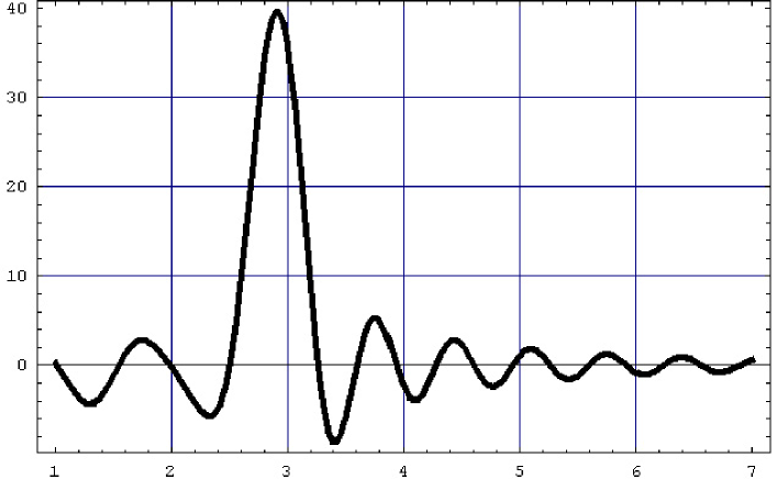
Fig. 1: Real part of the amplitude $e\rightarrow\gamma+e$ for the pulse background

Thus, numerical calculations show that unlike the case of QED without background fields, the amplitude (2) is not zero if $\vec{p}=\vec{k}+\vec{q}$. This just ensures the obvious fact that electron accelerates under the action of the background field and emits photons.

The fact that the amplitude is not zero on mass–shell gives us a gauge invariant way of answering affirmatively on the question about the radiation on mass–shell, which was formulated before the equation (15). The Fig.1 shows the dependence of the real part of the integral (2) on $k_{0}$ for some fixed values of the other variables. It doesn’t matter what are their concrete values. For the concreteness we take $p_{0}=4$ and $q_{0}=1$. Compare this discussion with the one in the introduction.

It is worth stressing here that the amplitude (2) is not only non–zero on mass–shell, but as well is complex rather than pure imaginary, as it should be at the leading order in any theory with the unitary evolution operator. Hence, this fact rises the question to [9] on how in detail the unitarity condition is ensured after the regularization of the IR divergences.

Now if in the amplitude like (2) one of the electron legs, say that one, which is with the momentum $k$, will be off-shell, then its virtuality $\lambda$ will not depend on the momentum $q$ of the soft photon, because there is no simple $\delta$–function ensuring energy conservation in the corresponding vertex. The same is true for the total amplitude (2). Note that according to the Fig. 1 the delta function which was present in the vertices in the theory without background fields is now smeared and as the result the virtuality $\lambda$ of the matter particle is not directly related to the momentum $q$ of the photon. This shows that there is no factorization of the IR divergences in the conditions under study.

3 IR divergences in loops

In this section we show what kind of consequences one obtains even at the leading order in the case if IR divergences do not cancel out. To see them, let us derive the electron Green function in the external field. Green function for the field $\Psi(x)$ satisfies to the following equation:

$$(i\hbox to0.0pt{$\displaystyle\partial$\hss}/+e\hbox to0.0pt{$\displaystyle A$\hss}\,/+m)G(x_{2},x_{1})=\delta(x_{2},x_{1}).$$

Or in the formal operator representation:

$$G=(\hbox to0.0pt{$\displaystyle\Pi$\hss}/+m)^{-1},\quad{}\hbox to0.0pt{$\displaystyle\Pi$\hss}/=\hbox to0.0pt{$\displaystyle p$\hss}\,/+e\hbox to0.0pt{$\displaystyle A$\hss}\,/.$$ (20)

Here we understand Green function $G$ as an operator acting on the states $|x\rangle$, $p$ is the usual momentum operator [1]. So the Green function is $G(x_{2},x_{1})=\langle{}x_{2}|G|x_{1}\rangle$.

We can write $G$ in the integral form:

$$G=-i\int_{0}^{\infty}ds(\hbox to0.0pt{$\displaystyle\Pi$\hss}/-m)\exp\left[i(\hbox to0.0pt{$\displaystyle\Pi$\hss}/\,^{2}-m^{2})s\right].$$ (21)

Introducing the unitary evolution operator $U(s)=\exp(-iHs)=\exp(i\hbox to0.0pt{$\displaystyle\Pi$\hss}/\,^{2}s)$, we can write the Green function as:

$$G(x_{2},x_{1})=-i\int_{0}^{\infty}dse^{-im^{2}s}\langle{}x_{2}(0)|\hbox to0.0pt{$\displaystyle\Pi$\hss}/\,(s)-m|x_{1}(s)\rangle,$$

where $|x(s)\rangle=U(s)|x(0)\rangle$.

Evolution of the operators $\Pi_{\mu}$ and $x_{\mu}$ is as follows:

$$\left\{\begin{array}[]{lll}\dfrac{dx_{\mu}}{ds}=&-i[H,x_{\mu}]&=2\Pi_{\mu};\\ \\ \dfrac{d\Pi_{\mu}}{ds}=&-i[\Pi_{\mu},H]&=-2eF_{\mu\nu}\Pi^{\nu}+ie\partial^{\alpha}F_{\alpha\mu}-\dfrac{1}{2}\partial_{\mu}F^{\alpha\beta}\sigma_{\alpha\beta},\end{array}\right.$$ (22)

where $F_{\mu\nu}=\partial_{[\mu}A_{\nu]}$ – is the field strength tensor and $\sigma_{\alpha\beta}=i[\gamma_{\alpha},\gamma_{\beta}]/2$.

For the simplicity we will use the matrix notation (${\mathbf{X}}=\|x_{\mu}\|,\,{\mathbf{\Pi}}=\|\Pi_{\mu}\|\mbox{ etc.}$) for the operators:

$$\left\{\begin{array}[]{lll}\dot{{\mathbf{X}}}&=2{\mathbf{\Pi}};\\ \dot{{\mathbf{\Pi}}}&=-2e{\mathbf{F}}{\mathbf{\Pi}}-{\mathbf{B}}.\end{array}\right.$$ (23)

Now we can write the solution of these equations in symbolic form. We will separate sectors $(0,3)$ and $(1,2)$ because matrix ${\mathbf{F}}$ has only $F^{0}_{3}$ and $F^{3}_{0}$ nonzero components. From now on we will understand the background value of ${\mathbf{F}}$ as $2\times{2}$ matrix with components only in $(0,3)$-sector:

$${\mathbf{F}}=\left[\begin{array}[]{lll}0&F^{0}_{3}\\ F^{3}_{0}&0\end{array}\right].$$ (24)

Using these notations, we can write our symbolic solutions as:

$$(0,3)\mbox{-sector}$$

$${\mathbf{\Pi}}(s)=e^{-2e{\mathbf{F}}{}s}{\mathbf{\Pi}}(0)+\frac{1}{2e}{\mathbf{F}}^{-1}{\mathbf{B}};$$

$${\mathbf{X}}(s)-{\mathbf{X}}(0)=\frac{1}{e}{\mathbf{F}}^{-1}(1-e^{-2e{\mathbf{F}}{}s}){\mathbf{\Pi}}(0)+\frac{1}{e}{\mathbf{F}}^{-1}{\mathbf{B}}{}s;$$

(25)

$$(1,2)\mbox{-sector}$$

$${\mathbf{\Pi}}(s)={\mathbf{\Pi}}(0);$$

$${\mathbf{X}}(s)-{\mathbf{X}}(0)=2{\mathbf{\Pi}}(0)s.$$

Furthermore, the transformation function $\langle{}x_{2}(0)|x_{1}(s)\rangle$ can be characterized by the following equations:

$$i\partial_{s}\langle{}x^{\prime}(0)|x(s)\rangle = \langle{}x^{\prime}(0)|H|x(s)\rangle;$$

$$(i\partial_{\mu}+eA_{\mu}(x))\langle{}x^{\prime}(0)|x(s)\rangle = \langle{}x^{\prime}(0)|\Pi_{\mu}(s)|x(s)\rangle;$$ (26)

$$(-i\partial^{\prime}_{\mu}+eA_{\mu}(x^{\prime}))\langle{}x^{\prime}(0)|x(s)\rangle = \langle{}x^{\prime}(0)|\Pi_{\mu}(0)|x(s)\rangle.$$

The boundary condition is: $\lim_{s\rightarrow 0}\langle{}x^{\prime}(0)|x(s)\rangle=\delta(x^{\prime}-x)$.

To solve the first equation in (3) we need ${\mathbf{\Pi}}^{2}$ and $[{\mathbf{X}}(s),{\mathbf{X}}(0)]$:

$$(0,3)\mbox{ sector}:$$

$${\mathbf{\Pi}}^{2}=({\mathbf{X}}(s)-{\mathbf{X}}(0))\mathbb{K}({\mathbf{X}}(s)-{\mathbf{X}}(0))+\frac{{\mathbf{B}}{}s^{2}{\mathbf{B}}}{\sinh(e{\mathbf{F}}{}s)^{2}}$$

$$+\frac{e{\mathbf{B}}{\mathbf{F}}}{\sinh(e{\mathbf{F}}{}s)^{2}}({\mathbf{X}}(s)-{\mathbf{X}}(0))+\frac{{\mathbf{B}}{}\tanh(e{\mathbf{F}}{s})}{2}\left(1+\frac{s}{e{\mathbf{F}}}\right){\mathbf{B}},$$

$$[{\mathbf{X}}(s),{\mathbf{X}}(0)]=i\frac{1-e^{-2e{\mathbf{F}}{s}}}{e{\mathbf{F}}};$$ (27)

$$(1,2)\mbox{ sector}:$$

$${\mathbf{\Pi}}^{2}=({\mathbf{X}}(s)-{\mathbf{X}}(0))\frac{1}{4s^{2}}({\mathbf{X}}(s)-{\mathbf{X}}(0)),$$

$$[{\mathbf{X}}(s),{\mathbf{X}}(0)]=2is.$$

Here $\mathbb{K}:=e^{2}{\mathbf{F}}^{2}\sinh(e{\mathbf{F}}{}s)^{-2}/4$.

Now we can combine both sectors:

$$\dfrac{\langle{}x_{2}(0)|H|x_{1}(s)\rangle}{\langle{}x_{2}(0)|x_{1}(s)\rangle}= ({\mathbf{X}}_{1}-{\mathbf{X}}_{2})\tilde{\mathbb{K}}({\mathbf{X}}_{1}-{\mathbf{X}}_{2})+\frac{es}{\sinh(eEs)^{2}}{\mathbf{B}}({\mathbf{X}}_{1}-{\mathbf{X}}_{2})+$$

$$+\frac{1}{2}{\mathbf{B}}\tanh(eEs){\mathbf{F}}(1+\frac{s}{e{\mathbf{F}}}){\mathbf{B}}+$$

$$+\frac{i}{2s}\mbox{Tr}\Delta_{2}+ie\coth(eEs)\mbox{Tr}\Delta_{1}+\frac{2s^{2}}{\sinh(eEs)^{2}}{\mathbf{B}}{\mathbf{F}}^{-1}{\mathbf{B}},$$

where $\tilde{\mathbb{K}}:=\mathbb{K}+\Delta_{2}/4s^{2}$ and

$$\Delta_{1}=\left[\begin{array}[]{llll}1&0&0&0\\ 0&0&0&0\\ 0&0&0&0\\ 0&0&0&1\\ \end{array}\right],\quad\Delta_{2}=\left[\begin{array}[]{llll}0&0&0&0\\ 0&1&0&0\\ 0&0&1&0\\ 0&0&0&0\\ \end{array}\right].$$ (29)

For our purposes we need only terms which dominate in the IR limit $x^{0}_{1}-x_{2}^{0}\rightarrow\infty$.

The solution of the equation (3) is:

$$\langle{}x_{2}(0)|x_{1}(s)\rangle\simeq \exp\left[-\frac{i}{4}({\mathbf{X}}_{1}-{\mathbf{X}}_{2})(eE\coth(eEs)\Delta_{1}-\frac{1}{s}\Delta_{2})({\mathbf{X}}_{1}-{\mathbf{X}}_{2})\right.$$

$$\left.-\frac{i}{E}\left(s\coth(eEs)-\frac{1}{eE}\log[\sinh(eEs)]\right){\mathbf{B}}({\mathbf{X}}_{1}-{\mathbf{X}}_{2})\right].$$

As $\Delta{}x_{0}=x_{1}^{0}-x_{2}^{0}\rightarrow\infty$ the Green function behaves as:

$$G(x_{1}-x_{2})\propto -i\int_{0}^{\infty}dse^{-im^{2}s}\left[\left(\frac{E\coth(eEs)}{2}\gamma^{0}+\frac{1}{2}\gamma^{3}\right)\Delta{}x_{0}\right]\times$$

$$\exp\left[-\frac{i}{4}eE\coth(eEs)\Delta{}x_{0}^{2}-\frac{i}{E}\left(s\coth(eEs)\phantom{\frac{\log(\sinh(eEs))}{eE}}\right.\right.$$

$$\left.\left.-\frac{\log(\sinh(eEs))}{eE}\right)e\partial_{0}F_{03}\gamma^{0}\gamma^{3}\Delta{x_{0}}\right].$$

Numerical calculations show that the Green function (3) for the fermion in the background of the pulse electric field (1) is divergent as $\Delta{x_{0}}\rightarrow\infty$.

There are several points, which are worth stressing at this point. First, the Feynman propagator, and both the Green functions for in–in and in–out formalisms, in the external electric field have as well similar to (3) characteristic divergence as $\Delta{x_{0}}\rightarrow\infty$. Second, as is well known, the Green function for the fermions in the theory without external fields is vanishing as $\Delta{x_{0}}\rightarrow\infty$. Third, if the external field is magnetic, Green function as well is vanishing in the limit $\Delta{x_{0}}\rightarrow\infty$.

Because of the divergence of the Green function in question one can straightforwardly show that even the first loop diagrams, in the QED with the background field under consideration, do have IR divergences. E.g. even the electron self-energy diagram does have IR divergence. It is worth stressing that without background fields electron self–energy is IR finite.

The divergence in question means that renormalized electron mass in the background electric field is infinite if the IR cutoff is taken to zero, which shows that such a formulation of the second quantized interacting field theory in the electric field background has some unavoidable problems.

One could hope to cancel these loop IR divergences by dressing electron legs with photon legs [7] or by using observations of the Lee and Nauenberg [8]. However these procedures work only in the case when (see e.g. book of Bogolyubov and Shirkov)

$$\left\langle out\left|\hat{S}\right|in\right\rangle=1,$$ (32)

but in our case this does not happen because $|in\rangle\neq|out\rangle.$ So we clearly see problems with IR divergences in the standard formulation of QFT in background fields. Similar conclusions one can make for the QED in the constant (in space and time) background electric field. Apparently the situation is similar to the one with QFT on de Sitter space background [2], which is, in particular, the main reason why we have considered it here.

4 Discussion

As we have shown above, the standard formulation of the second quantized field theory with the background electric fields, which are capable to create pairs, shows several problems. One of the main problems among them is the non–cancellation of the IR divergences. In particular it means that electron self–energy is IR divergent and there is nothing which can cancel this divergence. Because the dressing method of Bloch and Nordsiek does not work in the case if $|in\rangle\neq|out\rangle$. IR divergent electron self–energy means that electron has an infinite effective mass.

What kind of conclusions relevant for the back–reaction on the background fields can we draw out of these observations? Usually to take into account back–reaction it is tempting to act as follows [15]. To find the exact harmonics, define creation and annihilation operators for them, and then — define the vacuum $|in,0\rangle$ corresponding to the absence of the positive energy exact in–harmonics. This is supposed to be the initial state for the problem in question. We should evolve this state with the use of the exact QED Hamiltonian in the background field. This way it is tempting to define the rate of the decay of the background field as follows [15]. One should find the evolution of the initial state in question:

$$\left|\Psi,t\right\rangle={\rm T}e^{-i\int_{0}^{t}\hat{H}_{QED}(E)\,dt}\left|in,0\right\rangle.$$ (33)

Or one could use the functional integral counterpart of this wave functional. Here $t=0$ is the moment when the constant background electric field was set up, $t$ is the moment of observation, $\hat{H}_{QED}(E)$ is the full QED Hamiltonian corresponding to the exact harmonics, i.e. formulated in the background electric field $E$. Then one can use this wave functional to find the created background electric charge whose field compensates the originally present background electric field [15]. This so called Schwinger’s in–in formalism in background fields is applicable only in the case if $E$ is changing slowly in time, i.e. when there is a slow pair production rate otherwise we can not use the exact harmonics in fixed background field.

We see that ${\rm T}e^{-i\int_{0}^{t}H_{QED}(E)\,dt}$ is a non–unitary evolution operator in the case of the background field carrying infinite amount of energy. But in general, even if the background field creates a finite number of pairs, the QED with the ${\rm T}e^{-i\int_{0}^{t}H_{QED}(E)\,dt}$ evolution operator is an ill defined theory due to the problems with the IR divergences if the time range is taken to infinity. The Schwinger’s method is widely believed to cure out these problems, because it deals with the finite time range $[0,t]$.

However, our point here is that using the exact harmonics over background fields in calculations of correlation functions of interacting field theories, one actually deals with non–closed systems and, as the result, obtains various problems. In particular the Schwinger’s method can not be applied when, the initial value of $E$ is much bigger than the Schwinger’s critical value and there is a cascade of pair creation. The way out is to close somehow the system under consideration. How to do that?

For the QED in the background electric field one can do the following. Let $|0\rangle$ be the Fock vacuum state in QED without any background fields. To obtain the coherent state which corresponds to the background field $\vec{E}(x)$, we act on the vacuum by the shift operator:

$$|\vec{E}\rangle=\exp\left[\-i\int{}d^{3}x\vec{E}(x)\,\hat{\vec{A}}(x)\right]|0\rangle.$$ (34)

Here $\vec{E}(x)$ is the background field whose only non–zero component is, say, $E_{z}=E(x)$. It is easy to see that:

$$\langle\vec{E}|\hat{F}_{0z}|\vec{E}\rangle=E(x).$$ (35)

To find the decay rate of the background field we should find the evolution of the state $|\vec{E}\rangle$ in time. As the result:

$$E(x,t)=\left\langle\vec{E}\left|e^{iH_{QED}\,t}\hat{F}_{0z}\,e^{-iH_{QED}\,t}\right|\vec{E}\right\rangle,$$ (36)

where $H_{QED}$ is the full interacting QED Hamiltonian without any background fields. I.e. one should always expand around the eventual stable vacuum configuration. The VEV in question will be calculated elsewhere [16].

We would like to acknowledge discussions with P.Buividovich, S.Gavrilov, I.Polyubin and P.Burda. The work was partially supported by the Federal Agency of Atomic Energy of Russian Federation and by the grant for scientific schools NSh-679.2008.2.

References

- [1] J. S. Schwinger, Phys. Rev. 82, 664 (1951).
- [2] E. T. Akhmedov and P. V. Buividovich, Phys. Rev. D 78, 104005 (2008) [arXiv:0808.4106 [hep-th]].
- [3] G. W. Gibbons and S. W. Hawking, Phys. Rev. D 15, 2738 (1977).
- [4] E. Mottola, Phys. Rev. D 31, 754 (1985).
- [5] S. Weinberg, Phys. Rev. 140, B516 (1965).
- [6] A. V. Smilga, ‘‘Infrared And Collinear Divergence In Field Theory,’’ ITEP-35-1985.
- [7] F.Bloch and A.Nordsiek, Phys. Rev, vol. 52, p. 54 (1937).
- [8] T. D. Lee and M. Nauenberg, Phys. Rev. 133, B1549 (1964).
- [9] E. S. Fradkin and D. M. Gitman, Fortsch. Phys. 29, 381 (1981). D. M. Gitman, E. S. Fradkin and S. M. Shvartsman, Fortsch. Phys. 36, 643 (1988). S. P. Gavrilov, D. M. Gitman and S. M. Shvartsman, Sov. Phys. J. 23, 257 (1980).
- [10] A.A. Grib, S.G. Mamaev, V.M. Mostepanenko, Quantum effects in strong external fields, Moscow, (1980).
- [11] N. B. Narozhnyi and A. I. Nikishov, Teor. Mat. Fiz. 26, 16 (1976). A. I. Nikishov, Teor. Mat. Fiz. 20, 48 (1974). A. I. Nikishov, Zh. Eksp. Teor. Fiz. 57, 1210 (1969).
- [12] D. M. Gitman and S. P. Gavrilov, Izv. Vuz. Fiz. 1, 94 (1977) S. P. Gavrilov, D. M. Gitman and S. M. Shvartsman, Yad. Fiz. 29, 1097 (1979). Yu. Y. Volfengaut, S. P. Gavrilov, D. M. Gitman and S. M. Shvartsman, Yad. Fiz. 33, 743 (1981). S. P. Gavrilov and D. M. Gitman, Sov. Phys. J. 25, 775 (1982). S. P. Gavrilov and D. M. Gitman, Phys. Rev. D 53, 7162 (1996) [arXiv:hep-th/9603152]. S. P. Gavrilov and D. M. Gitman, Phys. Rev. D 78, 045017 (2008) [arXiv:0709.1828 [hep-th]].
- [13] H. Bateman, A, Erdélyi, Higher transcendental functions, NY, (1953);
- [14] Tzuu-Fang Chyi at al., hep-th/9912134;
- [15] T. N. Tomaras, N. C. Tsamis and R. P. Woodard, Phys. Rev. D 62, 125005 (2000) [arXiv:hep-ph/0007166].
- [16] E.T. Akhmedov, P.A. Burda, to appear.