The tau constant of a metrized graph and its behavior under graph operations

Abstract.

This paper concerns the tau constant, which is an important invariant of a metrized graph, and which has applications to arithmetic properties of curves. We give several formulas for the tau constant, and show how it changes under graph operations including deletion of an edge, contraction of an edge, and union of graphs along one or two points. We show how the tau constant changes when edges of a graph are replaced by arbitrary graphs. We prove Baker and Rumely’s lower bound conjecture on the tau constant for several classes of metrized graphs.

1. Introduction

Metrized graphs, which are graphs equipped with a distance function on their edges, appear in many places in arithmetic geometry. R. Rumely [Ru] used metrized graphs to develop arithmetic capacity theory, contributing to local intersection theory for curves over non-archimedean fields. T. Chinburg and Rumely [CR] used metrized graphs to define their “capacity pairing”. Another pairing satisfying “desirable” properties is Zhang’s “admissible pairing on curves”, introduced by S. Zhang [Zh1]. Arakelov introduced an intersection pairing at infinity and used analysis on Riemann surfaces to derive global results. In the non-archimedean case, metrized graphs appear as the analogue of a Riemann surface. Metrized graphs and their invariants are studied in the articles [Zh1], [Zh2], [Fa], [C1], [C2].

Metrized graphs which arise as dual graphs of curves, and Arakelov Green’s functions $g_{\mu}(x,y)$ on the metrized graphs, play an important role in both of the articles [CR] and [Zh1]. Chinburg and Rumely worked with a canonical measure $\mu_{can}$ of total mass $1$ on a metrized graph $\Gamma$ which is the dual graph of the special fiber of a curve $C$. Similarly, Zhang [Zh1] worked with an “admissible measure” $\mu_{ad}$, a generalization of $\mu_{can}$, of total mass $1$ on $\Gamma$. The diagonal values $g_{\mu_{can}}(x,x)$ are constant on $\Gamma$. M. Baker and Rumely called this constant the “tau constant” of a metrized graph $\Gamma$, and denoted it by $\tau(\Gamma)$. They posed a conjecture (see Conjecture 2.13) concerning lower bound of $\tau(\Gamma)$. We call it Baker and Rumely’s lower bound conjecture.

In summer 2003 at UGA, an REU group lead by Baker and Rumely studied properties of the tau constant and the lower bound conjecture. Baker and Rumely [BR] introduced a measure valued Laplacian operator $\Delta$ which extends Laplacian operators studied earlier in the articles [CR] and [Zh1]. This Laplacian operator combines the “discrete” Laplacian on a finite graph and the “continuous” Laplacian $-f^{\prime\prime}(x)dx$ on ${\mathbb{R}}$. Later, Baker and Rumely [BR] studied harmonic analysis on metrized graphs. In terms of spectral theory, the tau constant is the trace of the inverse operator of $\Delta$, acting on functions $f$ for which $\int_{\Gamma}fd\mu_{can}=0$, when $\Gamma$ has total length $1$.

In this paper, we express the canonical measure $\mu_{can}$ on a metrized graph $\Gamma$ in terms of the voltage function $j_{x}(y,z)$ on $\Gamma$. Our main focus is to give a systematic study of how the tau constant behaves under common graph operations. We give new formulas for the tau constant, and show how it changes under graph operations such as the deletion of an edge, the contraction of an edge into its end points, identifying any two vertices, and extending or shortening one of the edge lengths of $\Gamma$. We define a new graph operation which we call “full immersion of a collection of given graphs into another graph” (see §4), and we show how the tau constant changes under this operation. We prove the lower bound conjecture for several classes of metrized graphs. We show how our formulas can be applied to compute the tau constant for various classes of metrized graphs, including those with vertex connectivity $1$ or $2$. The results here extend those obtained in [C1, Sections 2.4, 3.1, 3.2, 3.3, 3.4 and 3.5]. Further applications of these results can be found in the articles [C2], [C3], [C4], and [C5].

2. The tau constant and the lower bound conjecture

In this section, we first recall a few facts about metrized graphs, the canonical measure $\mu_{can}$ on a metrized graph $\Gamma$, the Laplacian operator $\Delta$ on $\Gamma$, and the tau constant $\tau(\Gamma)$ of $\Gamma$. Then we give a new expression for $\mu_{can}$ in terms of the voltage function and two arbitrary points $p$, $q$ in $\Gamma$. This enables us to obtain a new formula for the tau constant. We also show how the Laplacian operator $\Delta$ acts on the product of two functions.

A metrized graph $\Gamma$ is a finite connected graph equipped with a distinguished parametrization of each of its edges. One can find other definitions of metrized graphs in the articles [BR], [Zh1], [BF], and the references contained in those articles.

A metrized graph can have multiple edges and self-loops. For any given $p\in\Gamma$, the number of directions emanating from $p$ will be called the valence of $p$, and will be denoted by $\upsilon(p)$. By definition, there can be only finitely many $p\in\Gamma$ with $\upsilon(p)\not=2$.

For a metrized graph $\Gamma$, we will denote its set of vertices by $V(\Gamma)$. We require that $V(\Gamma)$ be finite and non-empty and that $p\in V(\Gamma)$ for each $p\in\Gamma$ if $\upsilon(p)\not=2$. For a given metrized graph $\Gamma$, it is possible to enlarge the vertex set $V(\Gamma)$ by considering more additional points of valence $2$ as vertices.

For a given graph $\Gamma$ with vertex set $V(\Gamma)$, the set of edges of $\Gamma$ is the set of closed line segments with end points in $V(\Gamma)$. We will denote the set of edges of $\Gamma$ by $E(\Gamma)$.

Let $v:=\#(V(\Gamma))$ and $e:=\#(E(\Gamma))$. We define the genus of $\Gamma$ to be the first Betti number $g:=e-v+1$ of the graph $\Gamma$. Note that the genus is a topological invariant of $\Gamma$. In particular, it is independent of the choice of the vertex set $V(\Gamma)$. Since $\Gamma$ is connected, $g(\Gamma)$ coincides with the cyclotomic number of $\Gamma$ in combinatorial graph theory.

We denote the length of an edge $e_{i}\in E(\Gamma)$ by $L_{i}$. The total length of $\Gamma$, which will be denoted by $\ell(\Gamma)$, is given by $\displaystyle\ell(\Gamma)=\sum_{i=1}^{e}L_{i}$.

Let $\Gamma$ be a metrized graph. If we scale each edge of $\Gamma$ by multiplying its length by $\frac{1}{\ell(\Gamma)}$, we obtain a new graph which is called normalization of $\Gamma$, and will be denoted $\Gamma^{N}$. Thus, $\ell(\Gamma^{N})=1$.

We will denote the graph obtained from $\Gamma$ by deletion of the interior points of an edge $e_{i}\in E(\Gamma)$ by $\Gamma-e_{i}$. An edge $e_{i}$ of a connected graph $\Gamma$ is called a bridge if $\Gamma-e_{i}$ becomes disconnected. If there is no such edge in $\Gamma$, it will be called a bridgeless graph.

As in the article [BR], ${\mathop{\rm Zh}}(\Gamma)$ will be used to denote the set of all continuous functions $f:\Gamma\rightarrow{\mathbb{C}}$ such that for some vertex set $V(\Gamma)$, $f$ is ${\mathcal{C}}^{2}$ on $\Gamma\backslash V(\Gamma)$ and $f^{\prime\prime}(x)\in L^{1}(\Gamma)$.

Baker and Rumely [BR] defined the following measure valued Laplacian on a given metrized graph. For a function $f\in{\mathop{\rm Zh}}(\Gamma)$,

(1) $$\Delta_{x}(f(x))=-f^{\prime\prime}(x)dx-\sum_{p\in V(\Gamma)}\bigg{[}\sum_{\vec{v}\hskip 1.42262pt\text{at}\hskip 1.42262ptp}d_{\vec{v}}f(p)\bigg{]}\delta_{p}(x),$$

See the article [BR] for details and for a description of the largest class of functions for which a measure valued Laplacian can be defined.

We will now clarify how the Laplacian operator acts on a product of functions. For any two functions $f(x)$ and $g(x)$ in ${\mathop{\rm Zh}}(\Gamma)$, we have $f(x)g(x)\in{\mathop{\rm Zh}}(\Gamma)$ and

$$\begin{split}\Delta_{x}(f(x)g(x))&=-\big{[}f^{\prime\prime}(x)g(x)+2f^{\prime}(x)g^{\prime}(x)+f(x)g^{\prime\prime}(x)\big{]}dx\\ &\hskip 14.22636pt-\sum_{p\in V(\Gamma)}\bigg{[}\sum_{\vec{v}\hskip 1.42262pt\text{at}\hskip 1.42262ptp}(f(p)d_{\vec{v}}g(p)+g(p)d_{\vec{v}}f(p)\bigg{]}\delta_{p}(x)\\ &=-g(x)f^{\prime\prime}(x)dx-\sum_{p\in V(\Gamma)}g(p)\bigg{[}\sum_{\vec{v}\hskip 1.42262pt\text{at}\hskip 1.42262ptp}d_{\vec{v}}f(p)\bigg{]}\delta_{p}(x)\\ &\hskip 14.22636pt-f(x)g^{\prime\prime}(x)dx-\sum_{p\in V(\Gamma)}f(p)\bigg{[}\sum_{\vec{v}\hskip 1.42262pt\text{at}\hskip 1.42262ptp}d_{\vec{v}}g(p)\bigg{]}\delta_{p}(x)-2f^{\prime}(x)g^{\prime}(x)dx\\ &=g(x)\Delta_{x}f(x)+f(x)\Delta_{x}g(x)-2f^{\prime}(x)g^{\prime}(x)dx.\end{split}$$

Thus, we have shown the following result:

Theorem 2.1.

For any $f(x)$ and $g(x)$ $\in{\mathop{\rm Zh}}(\Gamma)$, we have

$$\Delta_{x}(f(x)g(x))=g(x)\Delta_{x}f(x)+f(x)\Delta_{x}g(x)-2f^{\prime}(x)g^{\prime}(x)dx.$$

The following proposition shows that the Laplacian on ${\mathop{\rm Zh}}(\Gamma)$ is “self-adjoint”, and explains the choice of sign in the definition of $\Delta$. It is proved by a simple integration by parts argument.

Proposition 2.2.

[Zh1, Lemma 4.a][BR, Proposition 1.1] For every $f,g\in{\mathop{\rm Zh}}(\Gamma)$,

$$\begin{split}\int_{\Gamma}\overline{g}\,\Delta f&=\int_{\Gamma}f\,\overline{\Delta g},\quad\text{ Self-Adjointness of $\Delta$}\\ &=\int_{\Gamma}f^{\prime}(x)\overline{g^{\prime}(x)}dx\quad\text{ Green's Identity}.\end{split}$$

In the article [CR], a kernel $j_{z}(x,y)$ giving a fundamental solution of the Laplacian is defined and studied as a function of $x,y,z\in\Gamma$. For fixed $z$ and $y$ it has the following physical interpretation: when $\Gamma$ is viewed as a resistive electric circuit with terminals at $z$ and $y$, with the resistance in each edge given by its length, then $j_{z}(x,y)$ is the voltage difference between $x$ and $z$, when unit current enters at $y$ and exits at $z$ (with reference voltage 0 at $z$).

For any $x$, $y$, $z$ in $\Gamma$, the voltage function $j_{x}(y,z)$ on $\Gamma$ is a symmetric function in $y$ and $z$, and it satisfies $j_{x}(x,z)=0$ and $j_{x}(y,y)=r(x,y)$, where $r(x,y)$ is the resistance function on $\Gamma$. For each vertex set $V(\Gamma)$, $j_{z}(x,y)$ is continuous on $\Gamma$ as a function of $3$ variables. As the physical interpretation suggests, $j_{x}(y,z)\geq 0$ for all $x$, $y$, $z$ in $\Gamma$. For proofs of these facts, see the articles [CR], [BR, sec 1.5 and sec 6], and [Zh1, Appendix]. The voltage function $j_{z}(x,y)$ and the resistance function $r(x,y)$ on a metrized graph were also studied by Baker and Faber [BF].

Proposition 2.3.

[CR] For any $p,q,x\in\Gamma$, $\quad\Delta_{x}j_{p}(x,q)=\delta_{q}(x)-\delta_{p}(x)$.

In [CR, Section 2], it was shown that the theory of harmonic functions on metrized graphs is equivalent to the theory of resistive electric circuits with terminals. We now recall the following well known facts from circuit theory. They will be used frequently and implicitly in this paper and in the papers [C2], [C3], [C4]. The basic principle of circuit analysis is that if one subcircuit of a circuit is replaced by another circuit which has the same resistances between each pair of terminals as the original subcircuit, then all the resistances between the terminals of the original circuit are unchanged. The following subcircuit replacements are particularly useful:

Series Reduction: Let $\Gamma$ be a graph with vertex set $\{p,q,s\}$. Suppose that $p$ and $s$ are connected by an edge of length $A$, and that $s$ and $q$ are connected by an edge of length $B$. Let $\beta$ be a graph with vertex set $\{p,q\}$, where $p$ and $q$ are connected by an edge of length $A+B$. Then the effective resistance in $\Gamma$ between $p$ and $q$ is equal to the effective resistance in $\beta$ between $p$ and $q$. These are illustrated by the first two graphs in Figure 1.

Figure 1. Series and Parallel Reductions

Parallel Reduction: Suppose $\Gamma$ and $\beta$ be two graphs with vertex set $\{p,q\}$. Suppose $p$ and $q$ in $\Gamma$ are connected by two edges of lengths $A$ and $B$, respectively, and let $p$ and $q$ in $\beta$ be connected by an edge of length $\frac{AB}{A+B}$ (see the last two graphs in Figure 1). Then the effective resistance in $\Gamma$ between $p$ and $q$ is equal to the effective resistance in $\beta$ between $p$ and $q$.

Delta-Wye transformation: This is the one case where a mesh can be replaced by a star. Let $\Gamma$ be a triangular graph with vertices $p$, $q$, and $s$. Then, $\Gamma$ (with resistance function $r_{\Gamma}$) can be transformed to a Y-shaped graph $\beta$ (with resistance function $r_{\beta}$) so that $p,q,s$ become end points in $\beta$ and the following equivalence of resistances hold: $r_{\Gamma}(p,q)=r_{\beta}(p,q)$, $r_{\Gamma}(p,s)=r_{\beta}(p,s)$, $r_{\Gamma}(q,s)=r_{\beta}(q,s).$ Moreover, for the resistances $a$, $b$, $c$ in $\Gamma$, we have the resistances $\frac{bc}{a+b+c}$, $\frac{ac}{a+b+c}$, $\frac{ab}{a+b+c}$ in $\beta$, as illustrated by the first two graphs in Figure 2.

Wye-Delta transformation: This is the inverse Delta-Wye transformation, and is illustrated by the last two graphs in Figure 2.

Figure 2. Delta-Wye and Wye-Delta transformations

Star-Mesh transformation: An $n$-star shaped graph ( i.e. $n$ edges with one common point whose other end points are of valence $1$) can be transformed into a complete graph of $n$ vertices (which does not contain the common end point) so that all resistances between the remaining vertices remain unchanged. A more precise description is as follows:

Let $L_{1},L_{2},\cdots,L_{n}$ be the edges in an $n$-star shaped graph $\Gamma$ with common vertex $p$, where $L_{i}$ is the length of the edge connecting the vertices $q_{i}$ and $p$ (i.e., the resistance between the vertices $q_{i}$ and $p$. The star-mesh transformation applied to $\Gamma$ gives a complete graph $\Gamma^{c}$ on the set of vertices $q_{1},q_{2},\cdots,q_{n}$ with $\frac{n(n-1)}{2}$ edges. Let $L_{ij}$ be the length of the edge connecting the vertices $q_{i}$ and $q_{j}$ in $\Gamma^{c}$ for any $1\leq i<j\leq n$. Then $\displaystyle L_{ij}=L_{i}L_{j}\cdot\sum_{k=1}^{n}\frac{1}{L_{k}}.$ When $n=2$, the star-mesh transformation is identical to series reduction. When $n=3$, the star-mesh transformation is identical to the Wye-Delta transformation, and can be inverted by the Delta-Wye transformation. When $n\geq 4$, there is no inverse transformation for the star-mesh transformation. Figure 3 illustrates the case $n=6$. (For more details see [S] or [F-C]).

Figure 3. Star-Mesh transformations when $n=6$.

For any given $p$ and $q$ in $\Gamma$, we say that an edge $e_{i}$ is not part of a simple path from $p$ to $q$ if all walks starting at $p$, passing through $e_{i}$, and ending at $q$ must visit some vertex more than once. Another basic principle of circuit reduction is the following transformation:

The effective resistances between $p$ and $q$ in both $\Gamma$ and $\Gamma-e_{i}$ are the same if $e_{i}$ is not part of a simple path from $p$ to $q$. Therefore, such an edge $e_{i}$ can be deleted as far as the resistance between $p$ and $q$ is concerned.

For any real-valued, signed Borel measure $\mu$ on $\Gamma$ with $\mu(\Gamma)=1$ and $|\mu|(\Gamma)<\infty$, define the function $\displaystyle j_{\mu}(x,y)\ =\ \int_{\Gamma}j_{\zeta}(x,y)\,d\mu({\zeta}).$ Clearly $j_{\mu}(x,y)$ is symmetric, and is jointly continuous in $x$ and $y$. Chinburg and Rumely discovered in [CR] that there is a unique real-valued, signed Borel measure $\mu=\mu_{can}$ such that $j_{\mu}(x,x)$ is constant on $\Gamma$. The measure $\mu_{\mathop{\rm can}}$ is called the canonical measure. Baker and Rumely [BR] called the constant $\frac{1}{2}j_{\mu}(x,x)$ the tau constant of $\Gamma$ and denoted by $\tau(\Gamma)$. In terms of spectral theory, as shown in the article [BR], the tau constant $\tau(\Gamma)$ is the trace of the inverse of the Laplacian operator on $\Gamma$ with respect to $\mu_{can}$.

The following lemma gives another description of the tau constant. In particular, it implies that the tau constant is positive.

Lemma 2.4.

[BR, Lemma 14.4] For any fixed $y$ in $\Gamma$, $\displaystyle\tau(\Gamma)=\frac{1}{4}\int_{\Gamma}\big{(}\frac{\partial}{\partial x}r(x,y)\big{)}^{2}dx$.

The canonical measure is given by the following explicit formula:

Theorem 2.5.

[CR, Theorem 2.11] Let $\Gamma$ be a metrized graph. Suppose that $L_{i}$ is the length of edge $e_{i}$ and $R_{i}$ is the effective resistance between the endpoints of $e_{i}$ in the graph $\Gamma-e_{i}$, when the graph is regarded as an electric circuit with resistances equal to the edge lengths. Then we have

$$\mu_{\mathop{\rm can}}(x)\ =\ \sum_{p\in V(\Gamma)}(1-\frac{1}{2}\text{v}\hskip 1.42262pt(p))\,\delta_{p}(x)+\sum_{e_{i}\in E(\Gamma)}\frac{dx}{L_{i}+R_{i}},$$

where $\delta_{p}(x)$ is the Dirac measure.

Corollary 2.6.

[BR, Corollary 14.2] The measure $\mu_{\mathop{\rm can}}$ is the unique measure $\nu$ of total mass 1 on $\Gamma$ maximizing the integral $\iint_{\Gamma\times\Gamma}r(x,y)\,d\nu(x)\overline{d\nu(y)}.$

The following theorem expresses $\mu_{can}$ in terms of the resistance function:

Theorem 2.7.

[BR, Theorem 14.1] The measure $\mu_{can}(x)=\frac{1}{2}\Delta_{x}r(x,p)+\delta_{p}(x)$ is of total mass $1$ on $\Gamma$, which is independent of $p\in\Gamma$.

It is shown in [CR] that as a function of three variables, on each edge $j_{x}(p,q)$ is a quadratic function of $p$, $q$, $x$ and possibly with linear terms in $|x-p|$, $|x-q|$, $|p-q|$ if some of $p$, $q$, $x$ belong to the same edge. These can be used to show that $j_{x}(p,q)$ is differentiable for $x\in\Gamma\backslash\big{(}\{p,q\}\cup V(\Gamma)\big{)}$. Moreover, we have $j_{x}(p,q)\in Zh(\Gamma)$ for each $p$, $q$ and $x$ in $\Gamma$.

For any $x$, $p$ and $q$ in $\Gamma$, we can transform $\Gamma$ to an $Y$-shaped graph with the same resistances between $x$, $p$, and $q$ as in $\Gamma$ by applying a sequence of circuit reductions. The resulting graph is shown in Figure 4, with the corresponding voltage values on each segment.

Figure 4. Circuit reduction with reference to $3$ points $x$, $p$ and $q$.

Then by Figure 4, we have

(2) $$\begin{split}\\ r(p,x)=j_{p}(x,q)+j_{x}(p,q),\;\,r(q,x)=j_{q}(x,p)+j_{x}(p,q),\;\,r(p,q)=j_{q}(x,p)+j_{p}(x,q),\end{split}$$

so

(3) $$\begin{split}\Delta_{x}r(p,x)=\Delta_{x}j_{p}(x,q)&+\Delta_{x}j_{x}(p,q),\qquad\quad\Delta_{x}r(q,x)=\Delta_{x}j_{q}(x,p)+\Delta_{x}j_{x}(p,q),\\ &\Delta_{x}r(p,q)=\Delta_{x}j_{q}(x,p)+\Delta_{x}j_{p}(x,q)=0.\end{split}$$

Using these formulas, we can express $\mu_{can}$ in terms of the voltage function in the following way:

Theorem 2.8.

For any $p,q\in\Gamma$, $\quad 2\mu_{can}(x)=\Delta_{x}j_{x}(p,q)+\delta_{q}(x)+\delta_{p}(x)$.

Proof.

By Proposition 2.3 and Equation (3),

(4) $$\begin{split}\Delta_{x}r(x,p)=\Delta_{x}j_{x}(p,q)+\delta_{q}(x)-\delta_{p}(x).\end{split}$$

Hence, the result follows from Theorem 2.7. ∎

Let $e_{i}\in E(\Gamma)$ be an edge for which $\Gamma-e_{i}$ is connected, and let $L_{i}$ be the length of $e_{i}$. Suppose $p_{i}$ and $q_{i}$ are the end points of $e_{i}$, and $p\in\Gamma-e_{i}$. By applying circuit reductions, $\Gamma-e_{i}$ can be transformed into a $Y$-shaped graph with the same resistances between $p_{i}$, $q_{i}$, and $p$ as in $\Gamma-e_{i}$. The resulting graph is shown by the first graph in Figure 5, with the corresponding voltage values on each segment, where $\hat{j}_{x}(y,z)$ is the voltage function in $\Gamma-e_{i}$. Since $\Gamma-e_{i}$ has such a circuit reduction, $\Gamma$ has the circuit reduction shown in the second graph in Figure 5. Throughout this paper, we will use the following notation: $R_{a_{i},p}:=\hat{j}_{p_{i}}(p,q_{i})$, $R_{b_{i},p}:=\hat{j}_{q_{i}}(p_{i},p)$, $R_{c_{i},p}:=\hat{j}_{p}(p_{i},q_{i})$, and $R_{i}$ is the resistance between $p_{i}$ and $q_{i}$ in $\Gamma-e_{i}$. Note that $R_{a_{i},p}+R_{b_{i},p}=R_{i}$ for each $p\in\Gamma$. When $\Gamma-e_{i}$ is not connected, we set $R_{b_{i},p}=R_{i}=\infty$ and $R_{a_{i},p}=0$ if $p$ belongs to the component of $\Gamma-e_{i}$ containing $p_{i}$, and we set $R_{a_{i},p}=R_{i}=\infty$ and $R_{b_{i},p}=0$ if $p$ belongs to the component of $\Gamma-e_{i}$ containing $q_{i}$.

Figure 5. Circuit reduction of $\Gamma-e_{i}$ with reference to $p_{i}$, $q_{i}$ and $p$.

Another description of the tau constant is given below.

Proposition 2.9.

[REU] Let $\Gamma$ be a metrized graph, and let $L_{i}$ be the length of the edge $e_{i}$, for $i\in\{1,2,\dots,e\}$. Using the notation above, if we fix a vertex $p$ we have

$$\tau(\Gamma)=\frac{1}{12}\sum_{e_{i}\in\Gamma}\left(\frac{L_{i}^{3}+3L_{i}(R_{a_{i},p}-R_{b_{i},p})^{2}}{(L_{i}+R_{i})^{2}}\right).$$

Here, if $\Gamma-e_{i}$ is not connected, i.e. $R_{i}$ is infinite, the summand corresponding to $e_{i}$ should be replaced by $3L_{i}$, its limit as $R_{i}\longrightarrow\infty$.

Proof.

We start by fixing a vertex point $p\in V(\Gamma)$. By applying circuit reductions, we can transform $\Gamma$ to the graph as in the second graph in Figure 5 when $x\in e_{i}$. Then, applying parallel reduction gives

$$r(x,p)=\frac{(x+R_{a_{i},p})(L_{i}-x+R_{b_{i},p})}{L_{i}+R_{i}}+R_{c_{i},p}.$$

Thus,

(5) $${\frac{d}{dx}}r(x,p)=\begin{cases}\frac{L_{i}-2x+R_{b_{i},p}-R_{a_{i},p}}{L_{i}+R_{i}},&\,\text{if }\,\Gamma-e_{i}\,\text{is connected},\\ \epsilon,&\,\text{if }\,\Gamma-e_{i}\,\text{is disconnected},\end{cases}$$

where $\epsilon$ is $+1$ or $-1$, depending on which component of $\Gamma-e_{i}$ the point $p$ belongs to.

By Lemma 2.4,

(6) $$\begin{split}\tau(\Gamma)=\frac{1}{4}\int_{\Gamma}\big{(}{\frac{d}{dx}}r(x,p)\big{)}^{2}dx=\frac{1}{4}\sum_{e_{i}\in\,E(\Gamma)}\int_{e_{i}}\big{(}{\frac{d}{dx}}r(x,p)\big{)}^{2}dx.\end{split}$$

Computing the integral after substituting Equation (5) into Equation (6) gives the result. ∎

Chinburg and Rumely showed in [CR, page 26] that

(7) $$\sum_{e_{i}\in E(\Gamma)}\frac{L_{i}}{L_{i}+R_{i}}=g,\quad\text{equivalently }\sum_{e_{i}\in E(\Gamma)}\frac{R_{i}}{L_{i}+R_{i}}=v-1.$$

Remark 2.10.

Valence Property of $\tau(\Gamma)$ Let $\Gamma$ be any metrized graph with resistance function $r(x,y)$. The formula for $\tau(\Gamma)$ given in Proposition 2.9 is independent of the chosen point $p\in V(\Gamma)$, where $V(\Gamma)$ is the specified vertex set. In particular, enlarging $V(\Gamma)$ by including points $p\in\Gamma$ with $\upsilon(p)=2$ does not change $\tau(\Gamma)$. Thus, $\tau(\Gamma)$ depends only on the topology and the edge length distribution of the metrized graph $\Gamma$.

Let $\Gamma$ be a metrized graph with $e$ edges. Then $\displaystyle\sum_{p\in V(\Gamma)}\upsilon(p)=2e$. This is the “Handshaking Lemma” of graph theory.

Remark 2.11.

By Proposition 2.9, for any $p$ and $q$ in $V(\Gamma)$,

$$\sum_{e_{i}\in\,E(\Gamma)}\frac{L_{i}(R_{a_{i},p}-R_{b_{i},p})^{2}}{(L_{i}+R_{i})^{2}}=\sum_{e_{i}\in\,E(\Gamma)}\frac{L_{i}(R_{a_{i},q}-R_{b_{i},q})^{2}}{(L_{i}+R_{i})^{2}}.$$

Let $\Gamma$ be a graph and let $p\in V(\Gamma)$. If a vertex $p$ is an end point of an edge $e_{i}$, then we write $e_{i}\sim p$. Since one of $R_{a_{i},p}$ and $R_{b_{i},p}$ is $0$ and the other is $R_{i}$ for every edge $e_{i}\sim p$,

(8) $$\sum_{e_{i}\in\,E(\Gamma)}\frac{L_{i}(R_{a_{i},p}-R_{b_{i},p})^{2}}{(L_{i}+R_{i})^{2}}=\sum_{\begin{subarray}{c}e_{i}\sim p\\ e_{i}\in\,E(\Gamma)\end{subarray}}\frac{L_{i}R_{i}^{2}}{(L_{i}+R_{i})^{2}}+\sum_{\begin{subarray}{c}e_{i}\not\sim p\\ e_{i}\in\,E(\Gamma)\end{subarray}}\frac{L_{i}(R_{a_{i},p}-R_{b_{i},p})^{2}}{(L_{i}+R_{i})^{2}}.$$

Lemma 2.12.

Let $\Gamma$ be a graph and $p\in V(\Gamma)$. Then

$$\begin{split}\sum_{e_{i}\in\,E(\Gamma)}\frac{L_{i}(R_{a_{i},p}-R_{b_{i},p})^{2}}{(L_{i}+R_{i})^{2}}=\frac{2}{v}\sum_{e_{i}\in\,E(\Gamma)}\frac{L_{i}R_{i}^{2}}{(L_{i}+R_{i})^{2}}+\frac{1}{v}\sum_{p\in\,V(\Gamma)}\Bigg{(}\sum_{\begin{subarray}{c}e_{i}\not\sim p\\ e_{i}\in\,E(\Gamma)\end{subarray}}\frac{L_{i}(R_{a_{i},p}-R_{b_{i},p})^{2}}{(L_{i}+R_{i})^{2}}\Bigg{)}.\end{split}$$

Proof.

By Remark 2.11, summing up Equation (8) over all $p\in V(\Gamma)$ and dividing by $v=\#(V(\Gamma))$ gives

(9) $$\begin{split}\sum_{e_{i}\in\,E(\Gamma)}\frac{L_{i}(R_{a_{i},p}-R_{b_{i},p})^{2}}{(L_{i}+R_{i})^{2}}&=\frac{1}{v}\sum_{p\in\,V(\Gamma)}\Bigg{(}\sum_{\begin{subarray}{c}e_{i}\sim p\\ e_{i}\in\,E(\Gamma)\end{subarray}}\frac{L_{i}R_{i}^{2}}{(L_{i}+R_{i})^{2}}\Bigg{)}\\ &\qquad+\frac{1}{v}\sum_{p\in\,V(\Gamma)}\Bigg{(}\sum_{\begin{subarray}{c}e_{i}\not\sim p\\ e_{i}\in\,E(\Gamma)\end{subarray}}\frac{L_{i}(R_{a_{i},p}-R_{b_{i},p})^{2}}{(L_{i}+R_{i})^{2}}\Bigg{)}.\end{split}$$

Each edge that is not a self loop is incident on exactly two vertices. On the other hand, $R_{i}=R_{a_{i},p}=R_{b_{i},p}=0$ for an edge $e_{i}$ that is a self loop. Thus, the result follows from Equation (9). ∎

It was shown in [BR, Equation 14.3] that for a metrized graph $\Gamma$ with $e$ edges, we have

(10) $$\frac{1}{16e}\ell(\Gamma)\ \leq\ \tau(\Gamma)\ \leq\ \frac{1}{4}\ell(\Gamma)\ ,$$

with equality in the upper bound if and only if $\Gamma$ is a tree. However, the lower bound is not sharp, and Baker and Rumely posed the following lower bound conjecture:

Conjecture 2.13.

[BR] There is a universal constant $C>0$ such that for all metrized graphs $\Gamma$,

$$\tau(\Gamma)\ \geq\ C\cdot\ell(\Gamma)\ .$$

Remark 2.14.

As can be seen from the examples and the cases we consider later in this paper, there is good evidence that $C=\frac{1}{108}$.

Remark 2.15.

[BR] If we multiply all lengths on $\Gamma$ by a positive constant $c$, we obtain a graph $\Gamma^{\prime}$ of total length $c\cdot\ell(\Gamma)$. Then $\tau(\Gamma^{\prime})=c\cdot\tau(\Gamma)$. This will be called the scale-independence of the tau constant. By this property, to prove Conjecture 2.13, it is enough to consider metrized graphs with total length $1$.

The following proposition gives an explicit formula for the tau constant for complete graphs, for which Conjecture 2.13 holds with $C=\frac{23}{500}$.

Proposition 2.16.

Let $\Gamma$ be a complete graph on $v$ vertices with equal edge lengths. Suppose $v\geq 2$. Then we have

(11) $$\begin{split}\tau(\Gamma)=\Big{(}\frac{1}{12}\big{(}1-\frac{2}{v}\big{)}^{2}+\frac{2}{v^{3}}\Big{)}\ell(\Gamma).\end{split}$$

In particular, $\tau(\Gamma)\geq\frac{23}{500}\ell(\Gamma)$, with equality when $v=5$.

Proof.

Let $\Gamma$ be a complete graph on $v$ vertices. If $v=2$, then $\Gamma$ contains only one edge $e_{1}$ of length $L_{1}$, i.e. $\Gamma$ is a line segment. In this case, $R_{1}$ is infinite. Therefore, $\tau(\Gamma)=\frac{L_{1}}{4}$ by Proposition 2.9, which coincides with Equation (11). Suppose $v\geq 3$. Then the valence of any vertex is $v-1$, so by basic graph theory $e=\frac{v(v-1)}{2}$, and $g=\frac{(v-1)(v-2)}{2}$. Since all edge lengths are equal, $L_{i}=\frac{\ell(\Gamma)}{e}$ for each edge $e_{i}\in E(\Gamma)$. By the symmetry of the graph, we have $R_{i}=R_{j}$ for any two edges $e_{i}$ and $e_{j}$ of $\Gamma$. Thus Equation (7) implies that $R_{i}=\frac{2L_{i}}{v-2}$ for each edge $e_{i}$. Moreover, by the symmetry of the graph again, $r(p,q)=\frac{L_{i}R_{i}}{L_{i}+R_{i}}$ for all distinct $p$, $q\in V(\Gamma)$. Again by the symmetry and the fact that $R_{a_{i},p}+R_{b_{i},p}=R_{i}$, we have $R_{a_{i},p}=R_{b_{i},p}=\frac{R_{i}}{2}$ for each edge $e_{i}$ with end points different from $p$. Substituting these values into the formula for $\tau(\Gamma)$ given in Proposition 2.9 and using Lemma 2.12 gives the equality. The inequality $\tau(\Gamma)\geq\frac{23}{500}\ell(\Gamma)$ now follows by elementary calculus. ∎

For a circle graph, Conjecture 2.13 holds with $C=\frac{1}{12}$.

Corollary 2.17.

Let $\Gamma$ be a circle graph. Then we have $\tau(\Gamma)=\frac{\ell(\Gamma)}{12}.$

Proof.

A circle graph can be considered as a complete graph on $3$ vertices. The vertices are of valence two, so by the valence property of $\Gamma$, edge length distribution does not effect the tau constant of $\Gamma$. If we position the vertices equally spaced on $\Gamma$, we can apply Proposition 2.16 with $v=3$. ∎

The following theorem is frequently needed in computations related to the tau constant. It is also interesting in its own right.

Theorem 2.18.

For any p, q $\in\Gamma$ and $-1<n\in{\mathbb{R}}$,

$$\int_{\Gamma}(\frac{d}{dx}j_{p}(x,q))^{2}j_{p}(x,q)^{n}dx=\frac{1}{n+1}r(p,q)^{n+1}.$$

Proof.

Note that $j_{p}(x,q)^{n+1}\in{\mathop{\rm Zh}}(\Gamma)$ when $-1<n\in{\mathbb{R}}$.

$$\begin{split}(n+1)\int_{\Gamma}(\frac{d}{dx}j_{p}(x,q))^{2}j_{p}(x,q)^{n}dx&=\int_{\Gamma}\frac{d}{dx}j_{p}(x,q)\frac{d}{dx}(j_{p}(x,q)^{n+1})dx\\ &=\int_{\Gamma}j_{p}(x,q)^{n+1}\Delta_{x}j_{p}(x,q),\quad\text{by Proposition~{}\ref{prop Greens identity}}\\ &=\int_{\Gamma}j_{p}(x,q)^{n+1}(\delta_{q}(x)-\delta_{p}(x)).\end{split}$$

Then the result follows from the properties of the voltage function. ∎

We isolate the cases $n=0,\,1$, and $2$, since we will use them later on.

Corollary 2.19.

For any $p$ and $q$ in $\Gamma$,

$$\int_{\Gamma}(\frac{d}{dx}j_{p}(x,q))^{2}dx=r(p,q),\quad\quad\int_{\Gamma}(\frac{d}{dx}j_{p}(x,q))^{2}j_{p}(x,q)dx=\frac{1}{2}r(p,q)^{2}\quad\text{and}$$

$$\int_{\Gamma}(\frac{d}{dx}j_{p}(x,q))^{2}j_{p}(x,q)^{2}dx=\frac{1}{3}r(p,q)^{3}.$$

Lemma 2.20.

For any $p,q,x\in\Gamma$,

$$\begin{split}\int_{\Gamma}{\frac{d}{dx}}j_{x}(p,q){\frac{d}{dx}}j_{p}(x,q)dx=\int_{\Gamma}j_{p}(x,q)\Delta_{x}j_{x}(p,q)=\int_{\Gamma}j_{x}(p,q)\Delta_{x}j_{p}(x,q)=0.\end{split}$$

Proof.

Since $\Delta_{x}$ is a self-adjoint operator (see Proposition 2.2),

$$\int_{\Gamma}j_{p}(x,q)\Delta_{x}j_{x}(p,q)=\int_{\Gamma}j_{x}(p,q)\Delta_{x}j_{p}(x,q)=j_{p}(p,q)-j_{q}(p,q)=0,$$

where the second equality is by Proposition 2.3. Also, by the Green’s identity (see Proposition 2.2), $\int_{\Gamma}j_{x}(p,q)\Delta_{x}j_{p}(x,q)=\int_{\Gamma}{\frac{d}{dx}}j_{p}(x,q){\frac{d}{dx}}j_{x}(p,q)dx.$ This completes the proof. ∎

Now we are ready to express the tau constant in terms of the voltage function.

Theorem 2.21.

For any $p,q\in\Gamma$, $\tau(\Gamma)=\frac{1}{4}\int_{\Gamma}(\frac{d}{dx}j_{x}(p,q))^{2}dx+\frac{1}{4}r(p,q).$

Proof.

For any $p,\,q\in\Gamma$, we have

$$\begin{split}4\tau(\Gamma)&=\int_{\Gamma}\big{(}\frac{\partial}{\partial x}r(p,x)\big{)}^{2}dx,\quad\text{by Lemma~{}\ref{lemtauformula};}\\ &=\int_{\Gamma}r(p,x)\Delta_{x}r(p,x),\quad\text{by the Green's identity;}\\ &=\int_{\Gamma}r(p,x)\big{(}\Delta_{x}j_{x}(p,q)+\delta_{q}(x)-\delta_{p}(x)\big{)},\quad\text{by Equation~{}(\ref{eqn lem can jpq});}\\ &=\int_{\Gamma}r(p,x)\Delta_{x}j_{x}(p,q)+r(p,q),\quad\text{since $r(p,p)=0$;}\\ &=\int_{\Gamma}(j_{x}(p,q)+j_{p}(x,q))\Delta_{x}j_{x}(p,q)+r(p,q),\quad\text{by Equation~{}(\ref{eqn1.1});}\\ &=\int_{\Gamma}(\frac{d}{dx}j_{x}(p,q))^{2}dx+\int_{\Gamma}j_{x}(p,q)\Delta_{x}j_{p}(x,q)+r(p,q),\quad\text{by Proposition~{}\ref{prop Greens identity};}\\ &=\int_{\Gamma}(\frac{d}{dx}j_{x}(p,q))^{2}dx+r(p,q),\quad\text{by Lemma~{}\ref{lemorthogonality}}.\end{split}$$

This is what we wanted to show. ∎

Since $j_{x}(p,p)=r(p,x)$ and $r(p,p)=0$, Lemma 2.4 is the special case of Theorem 2.21 with $q=p$.

Suppose $\Gamma$ is a graph which is the union of two subgraphs $\Gamma_{1}$ and $\Gamma_{2}$, i.e., $\Gamma=\Gamma_{1}\cup\Gamma_{2}$. If $\Gamma_{1}$ and $\Gamma_{2}$ intersect in a single point $p$, i.e., $\Gamma_{1}\cap\Gamma_{2}=\{p\}$, then by circuit theory (see also [BF, Theorem 9 (ii)]) we have $r(x,y)=r(x,p)+r(p,y)$ for each $x\in\Gamma_{1}$ and $y\in\Gamma_{2}$. By using this fact and Corollary 2.4, we obtain $\tau(\Gamma_{1}\cup\Gamma_{2})=\tau(\Gamma_{1})+\tau(\Gamma_{2})$, which we call the “additive property” of the tau constant. It was initially noted in [REU].

The following corollary of Theorem 2.21 was given in [BR, Equation 14.3].

Corollary 2.22.

Let $\Gamma$ be a tree, i.e. a graph without cycles. Then, $\tau(\Gamma)=\frac{\ell(\Gamma)}{4}$.

Proof.

First we note that for a line segment $\beta$ with end points $p$ and $q$, we have that $r(p,q)=\ell(\beta)$. It is clear by circuit theory that $j_{x}(p,q)=0$ for any $x\in\beta$, where $j_{x}(y,z)$ is the voltage function on $\beta$. Therefore, $\tau(\beta)=\frac{\ell(\beta)}{4}$ by Theorem 2.21. Hence the result follows for any tree graph by applying the additive property whenever it is needed. ∎

Thus, Conjecture 2.13 holds with $C=\frac{1}{4}$ for a tree graph.

Corollary 2.23.

Let $\Gamma$ be a metrized graph, and let $E_{1}(\Gamma)=\{e_{i}\in E(\Gamma)|\text{$e_{i}$ is a bridge}\}.$ Suppose $\overline{\Gamma}$ is the metrized graph obtained from $\Gamma$ by contracting edges in $E_{1}(\Gamma)$ to their end points. Then $\tau(\Gamma)=\tau(\overline{\Gamma})+\frac{\ell(\Gamma)-\ell(\overline{\Gamma})}{4}$.

Proof.

If $E_{1}(\Gamma)\not=\emptyset$, we successively apply the additive property of the tau constant and Corollary 2.22 to obtain the result. ∎

By Corollary 2.23, to prove Conjecture 2.13, it is enough to prove it for bridgeless graphs.

Theorem 2.24 (Baker).

Suppose all edge lengths in a metrized graph $\Gamma$ with $\ell(\Gamma)=1$ are equal, i.e., of length $\frac{1}{e}$. Then $\tau(\Gamma)\geq\frac{1}{12}(\frac{g}{e})^{2}$. In particular, Conjecture 2.13 holds with $C=\frac{1}{108}$ if we also have $\upsilon(p)\geq 3$ for each vertex $p\in V(\Gamma)$.

Proof.

By Corollary 2.23, the scale-independence and the additive properties of $\tau(\Gamma)$, it will be enough to prove the result for a graph $\Gamma$ that does not have any edge whose removal disconnects it. Applying the Cauchy-Schwarz inequality to the second part of the equality $\displaystyle\sum_{e_{i}\in E(\Gamma)}\frac{L_{i}^{3}}{(L_{i}+R_{i})^{2}}=\sum_{e_{i}\in E(\Gamma)}\frac{L_{i}^{3}}{(L_{i}+R_{i})^{2}}\sum_{e_{i}\in E(\Gamma)}L_{i}$ gives

(12) $$\begin{split}\sum_{e_{i}\in E(\Gamma)}\frac{L_{i}^{3}}{(L_{i}+R_{i})^{2}}\geq\Big{(}\sum_{e_{i}\in E(\Gamma)}\frac{L_{i}^{2}}{L_{i}+R_{i}}\Big{)}^{2}.\end{split}$$

We have

$$\begin{split}\tau(\Gamma)&\geq\frac{1}{12}\sum_{e_{i}\in E(\Gamma)}\frac{L_{i}^{3}}{(L_{i}+R_{i})^{2}},\quad\text{by Proposition~{}\ref{proptau}};\\ &\geq\frac{1}{12}\Big{(}\sum_{e_{i}\in E(\Gamma)}\frac{L_{i}^{2}}{L_{i}+R_{i}}\Big{)}^{2},\quad\text{by Equation~{}(\ref{eqnthmcauchy1})};\\ &=\frac{1}{12}\Big{(}\frac{1}{e}\sum_{e_{i}\in E(\Gamma)}\frac{L_{i}}{L_{i}+R_{i}}\Big{)}^{2},\quad\text{since all edge lengths are equal;}\\ &=\frac{1}{12}(\frac{g}{e})^{2},\quad\text{by Equation~{}(\ref{eqn genus})}.\end{split}$$

This proves the first part. If $\upsilon(p)\geq 3$ for each $p\in V(\Gamma)$, then we have $e\geq\frac{3}{2}v$ by basic properties of connected graphs. Thus $g=e-v+1\geq e-\frac{2}{3}e+1\geq\frac{e}{3}$. Using this inequality along with the first part gives the last part. ∎

In the next theorem, we show that Conjecture 2.13 holds for another large class of graphs with $C=\frac{1}{48}$. First, we recall Jensen’s Inequality:

For any integer $n\geq 2$, let $a_{i}\in(c,d)$, an interval in ${\mathbb{R}}$, and $b_{i}\geq 0$ for all $i=1,\dots,n$. If $f$ is a convex function on the interval $(c,d)$, then

$$f\Big{(}\frac{\sum_{i=1}^{n}b_{i}a_{i}}{\sum_{i=1}^{n}b_{i}}\Big{)}\leq\frac{\sum_{i=1}^{n}b_{i}f(a_{i})}{\sum_{i=1}^{n}b_{i}}.$$

The inequality is reversed, if $f$ is a concave function on $(c,d)$.

Theorem 2.25.

Let $\Gamma$ be a graph with $\ell(\Gamma)=1$ and let $L_{i}$, $R_{i}$ be as before. Then we have $\tau(\Gamma)\geq\frac{1}{12}\frac{1}{\big{(}1+\sum_{e_{i}\in E(\Gamma)}R_{i}\big{)}^{2}}.$ In particular, if any pair of vertices $p_{i}$ and $q_{i}$ that are end points of an edge are joined by at least two edges, we have $\tau(\Gamma)\geq\frac{1}{48}.$

Proof.

Let $b_{i}=L_{i}$, $a_{i}=\frac{L_{i}+R_{i}}{L_{i}}$, and $f(x)=\frac{1}{x}$ on $(0,\infty)$. Then applying Jensen’s inequality and using the assumption that $\sum b_{i}=\ell(\Gamma)=1$, we obtain the following inequality:

(13) $$\begin{split}\sum_{e_{i}\in E(\Gamma)}\frac{L_{i}^{2}}{L_{i}+R_{i}}\geq\frac{1}{1+\sum_{e_{i}\in E(\Gamma)}R_{i}}.\end{split}$$

Then the first part follows from Proposition 2.9, Equation (12), and Equation (13). Under the assumptions of the second part, we obtain $\sum_{e_{i}\in E(\Gamma)}R_{i}\leq\sum_{e_{i}\in E(\Gamma)}L_{i}=1$ by applying parallel circuit reduction. This yields the second part. ∎

Additional proofs of Equation (13) can be found in [C1, page 50].

Theorem 2.26.

Let $\Gamma$ be a metrized graph with $\ell(\Gamma)=1$. Then we have

$$\sum_{e_{i}\in\,E(\Gamma)}\frac{L_{i}R_{i}^{2}}{(L_{i}+R_{i})^{2}}\geq\Big{(}\sum_{e_{i}\in\,E(\Gamma)}\frac{L_{i}R_{i}}{L_{i}+R_{i}}\Big{)}^{2}.$$

Proof.

We have $\ell(\Gamma)=1$. Hence, by Cauchy-Schwarz inequality

$$\sum_{e_{i}\in E(\Gamma)}\frac{L_{i}R_{i}^{2}}{(L_{i}+R_{i})^{2}}=\sum_{e_{i}\in E(\Gamma)}\frac{L_{i}R_{i}^{2}}{(L_{i}+R_{i})^{2}}\sum_{e_{i}\in E(\Gamma)}L_{i}\geq\Big{(}\sum_{e_{i}\in E(\Gamma)}\frac{L_{i}R_{i}}{L_{i}+R_{i}}\Big{)}^{2}.$$

∎

The following theorem improves Theorem 2.24 slightly:

Theorem 2.27.

Suppose all edge lengths in a graph $\Gamma$ with $\ell(\Gamma)=1$ are equal, i.e., of length $\frac{1}{e}$. Then $\tau(\Gamma)\geq\frac{1}{12}(\frac{g}{e})^{2}+\frac{1}{2v}(\frac{v-1}{e})^{2}$.

Proof.

It follows from Lemma 2.12 and Theorem 2.26 that

$$\sum_{e_{i}\in\,E(\Gamma)}\frac{L_{i}(R_{a_{i},p}-R_{b_{i},p})^{2}}{(L_{i}+R_{i})^{2}}\geq\frac{2}{v}\big{(}\sum_{e_{i}\in\,E(\Gamma)}\frac{L_{i}R_{i}}{L_{i}+R_{i}}\big{)}^{2}.$$

Since $L_{i}=\frac{1}{e}$ for each edge $e_{i}$, $\sum_{e_{i}\in\,E(\Gamma)}\frac{L_{i}R_{i}}{L_{i}+R_{i}}=\frac{1}{e}\sum_{e_{i}\in\,E(\Gamma)}\frac{R_{i}}{L_{i}+R_{i}}=\frac{v-1}{e}$ by using Equation (7). Therefore, the result follows from Proposition 2.9 and the proof of Theorem 2.24. ∎

In the next section, we will derive explicit formulas for the tau constants of certain graphs with multiple edges.

3. The tau constants of metrized graphs with multiple edges

Let $\Gamma$ be an arbitrary graph; write $E(\Gamma)=\{e_{1},e_{2},\dots,e_{e}\}$. As before, let $L_{i}$ be the length of edge $e_{i}$. Let $\Gamma^{DA,n}$, for a positive integer $n\geq 2$, be the graph obtained from $\Gamma$ by replacing each edge $e_{i}\in E(\Gamma)$ by $n$ edges $e_{i,1},e_{i,2},\dots,e_{i,n}$ of equal lengths $\frac{L_{i}}{n}$. (Here DA stands for “Double Adjusted”.) Then, $V(\Gamma)=V(\Gamma^{DA,n})$ and $\ell(\Gamma)=\ell(\Gamma^{DA,n})$. We set $\Gamma^{DA}:=\Gamma^{DA,2}$. The following observations will enable us to compute $\tau(\Gamma^{DA,n})$ in terms of $\tau(\Gamma)$.

We will denote by $R_{j}(\Gamma)$ the resistance between end points of an edge $e_{j}$ of a graph $\Gamma$ when the edge $e_{j}$ is deleted from $\Gamma$.

Figure 6 shows the edge replacement for an edge when $n=4$.

Figure 6. $\Gamma$ and $\Gamma^{DA,4}$

A graph with two vertices and $m$ edges connecting the vertices will be called a $m$-banana graph.

Lemma 3.1.

Let $\beta$ be a $m$-banana graph, as shown in Figure 7, such that $L_{i}=L$ for each $e_{i}\in\beta$. Let $r(x,y)$ be the resistance function in $\beta$, and let $p$ and $q$ be the end points of all edges. Then, $r(p,q)=\frac{L}{m}.$

Proof.

By parallel circuit reduction, $\frac{1}{r(p,q)}=\sum_{k=1}^{m}\frac{1}{L}=\frac{m}{L}$. Hence, the result follows. ∎

Figure 7. Circuit reduction for a banana graph.

Remark 3.2.

If we divide each edge length of a graph $\Gamma$, with resistance function $r(x,y)$, by a positive number $k$, we obtain a graph with resistance function $\frac{r(x,y)}{k}$.

Corollary 3.3.

Let $r(x,y)$ and $r^{n}(x,y)$ be the resistance functions in $\Gamma$ and $\Gamma^{DA,n}$, respectively. Then, for any $p$ and $q$ $\in V(\Gamma)$, $r^{n}(p,q)=\frac{r(p,q)}{n^{2}}.$

Proof.

By using Lemma 3.1, every group of $n$ edges $e_{i,1},e_{i,2},\dots,e_{i,n}$, in $E(\Gamma^{DA,n})$, corresponding to edge $e_{i}\in E(\Gamma)$ can be transformed into an edge $e_{i}^{\prime}$. When completed, this process results in a graph which can also be obtained from $\Gamma$ by dividing each edge length $L_{i}$ by $n^{2}$. Therefore, the result follows from Remark 3.2. ∎

Theorem 3.4.

Let $\Gamma$ be any graph, and let $\Gamma^{DA,n}$ be the related graph described before. Then

$$\tau(\Gamma^{DA,n})=\frac{\tau(\Gamma)}{n^{2}}+\frac{\ell(\Gamma)}{12}\big{(}\frac{n-1}{n}\big{)}^{2}+\frac{n-1}{6n^{2}}\sum_{e_{i}\in\,E(\Gamma)}\frac{L_{i}^{2}}{L_{i}+R_{i}}.$$

Proof.

Let $p$ be a fixed vertex in $V(\Gamma)=V(\Gamma^{DA,n})$. Whenever $x\in e_{i,j}$ for some $j\in\{1,2,\dots,n\}$, we can transform the graph $\Gamma^{DA,n}$ to the graph as shown in Figure 8 by using Corollary 3.3, Corollary 3.3 and circuit reduction for $\Gamma-e_{i}$. (Here $R_{a_{i,p}}$, $R_{b_{i,p}}$ and $R_{c_{i,p}}$ are as in Proposition 2.9 and so $R_{a_{i,p}}+R_{b_{i,p}}=R_{i}$.)

Figure 8. Circuit reduction for $\Gamma^{DA,n}$ with reference to an edge and a point.

In Figure 8, we have $a=\frac{R_{a_{i,p}}(\Gamma)}{n^{2}},\,$ $b=\frac{R_{b_{i,p}}(\Gamma)}{n^{2}},\,$ $c=\frac{R_{c_{i,p}}(\Gamma)}{n^{2}}$, $A$ is the edge $e_{i,j}$ of length $\frac{L_{i}}{n}$, and $d=\frac{L_{i}}{n(n-1)}.$ Then, by using a Delta-Wye transformation followed by parallel circuit reduction, we derive the formula below for the effective resistance between a point $x\in e_{i,j}$ and $p$, which will be denoted by $r^{n}(x,p)$.

(14) $$r^{n}(x,p)=\frac{\big{(}x+\frac{ad}{a+b+d}\big{)}\big{(}\frac{L_{i}}{n}-x+\frac{db}{a+b+d}\big{)}}{\frac{L_{i}}{n}+\frac{ad+db}{a+b+d}}+\frac{ab}{a+b+d}+c.$$

By using Corollary 2.4,

(15) $$\begin{split}\tau(\Gamma^{DA,n})&=\frac{1}{4}\int_{\Gamma^{DA,n}}\left({\frac{d}{dx}}r(x,y)\right)^{2}dx.\\ &=\frac{1}{4}\sum_{e_{i,j}\in E(\Gamma^{DA,n})}\int_{e_{i,j}}\left({\frac{d}{dx}}r(x,y)\right)^{2}dx.\\ &=\frac{n}{4}\sum_{e_{i}\in E(\Gamma)}\int_{0}^{\frac{L_{i}}{n}}\left({\frac{d}{dx}}r(x,y)\right)^{2}dx,\quad\text{by symmetry within multiple edges.}\end{split}$$

This integral was computed using Maple, after substituting the derivative of Equation (14) and the values of $a$, $b$ and $d$ as above into Equation (15). Let

(16) $$\begin{split}I_{i}:=&\int_{0}^{\frac{L_{i}}{n}}\left({\frac{d}{dx}}r(x,y)\right)^{2}dx,\quad\text{and let}\\ J_{i}:=&\frac{L_{i}}{12}(\frac{n-1}{n})^{2}+\frac{n-1}{6n^{2}}\frac{L_{i}^{2}}{L_{i}+R_{i}}+\frac{1}{12n^{2}}\frac{L_{i}^{3}+3L_{i}(R_{a_{i,p}}-R_{b_{i,p}})^{2}}{(L_{i}+R_{i})^{2}}.\end{split}$$

Then, via Maple, $\frac{n}{4}I_{i}=J_{i}$. Inserting this into Equation (15) and using Proposition 2.9, we see that $\tau(\Gamma^{DA,n})=\sum_{e_{i}\in E(\Gamma)}J_{i}$. This yields the theorem. ∎

In §4, we will give a far-reaching generalization of Theorem 3.4.

Corollary 3.5.

Let $\Gamma$ be a graph. Then,

$$\begin{split}\tau(\Gamma^{DA})&=\frac{\tau(\Gamma)}{4}+\frac{\ell(\Gamma)}{48}+\frac{1}{24}\sum_{e_{i}\in\,E(\Gamma)}\frac{L_{i}^{2}}{L_{i}+R_{i}}.\\ \tau(\Gamma^{DA,3})&=\frac{\tau(\Gamma)}{9}+\frac{\ell(\Gamma)}{27}+\frac{1}{27}\sum_{e_{i}\in\,E(\Gamma)}\frac{L_{i}^{2}}{L_{i}+R_{i}}.\end{split}$$

Proof.

Setting $n=2$ and $n=3$ in Theorem 3.4 gives the equalities. ∎

Figure 9. $\Gamma\rightarrow\Gamma^{DA}$, doubling the edges.

Corollary 3.6.

Let $\Gamma$ be a banana graph with $n\geq 1$ edges that have equal length. Then,

$$\tau(\Gamma)=\frac{\ell(\Gamma)}{4n^{2}}+\frac{\ell(\Gamma)}{12}\big{(}\frac{n-1}{n}\big{)}^{2}=\frac{\ell(\Gamma)}{12}\frac{n^{2}-2n+4}{n^{2}}\geq\frac{\ell(\Gamma)}{16}.$$

Proof.

Let $\beta$ be a line segment of length $\ell(\Gamma)$. Since $R_{1}(\beta)=\infty$, $\tau(\beta^{DA,n})=\frac{\tau(\beta)}{n^{2}}+\frac{\ell(\beta)}{12}\big{(}\frac{n-1}{n}\big{)}^{2}+0$ by Theorem 3.4. On the other hand, we have $\beta^{DA,n}=\Gamma$, $\ell(\beta)=\ell(\Gamma)$, and $\tau(\beta)=\frac{\ell(\beta)}{4}$ since $\beta$ is a tree. This gives the equalities we want to show, and the inequality follows by Calculus. ∎

By dividing each edge $e_{i}\in E(\Gamma)$ into $m$ equal subsegments and considering the end points of the subsegments as new vertices, we obtain a new graph which we denote by $\Gamma^{m}$. Note that $\Gamma$ and $\Gamma^{m}$ have the same topology, and $\ell(\Gamma)=\ell(\Gamma^{m})$, but $\#(E(\Gamma^{m}))=m\cdot\#(E(\Gamma))=m\cdot e$ and $\#(V(\Gamma^{m}))=\#(V(\Gamma))+(m-1)\cdot\#(E(\Gamma))=v+(m-1)\cdot e$. Figure 10 shows an example when $\Gamma$ is a line segment with end points $p$ and $q$, and $m=3$.

Figure 10. Division into $m=3$ equal parts.

Suppose an edge $e_{k}\in E(\Gamma^{m})$ has end points $p_{k}$ and $q_{k}$ that are in $V(\Gamma^{m})$. To avoid any potential misinterpretation, we will denote the length of $e_{k}$ by $L_{k}(\Gamma^{m})$. Likewise, the resistance between $p_{k}$ and $q_{k}$ in $\Gamma^{m}-e_{k}$ will be denoted by $R_{k}(\Gamma^{m})$.

Lemma 3.7.

Let $\Gamma$ be a graph, and $\Gamma^{m}$ be as defined. Then the following identities hold:

$$\begin{split}&(i)\qquad\sum_{e_{k}\in E(\Gamma^{m})}\frac{L_{k}(\Gamma^{m})^{2}}{L_{k}(\Gamma^{m})+R_{k}(\Gamma^{m})}=\frac{1}{m}\sum_{e_{i}\in E(\Gamma)}\frac{L_{i}^{2}}{L_{i}+R_{i}}.\\ &(ii)\qquad\sum_{e_{k}\in E(\Gamma^{m})}\frac{L_{k}(\Gamma^{m})^{3}}{(L_{k}(\Gamma^{m})+R_{k}(\Gamma^{m}))^{2}}=\frac{1}{m^{2}}\sum_{e_{i}\in E(\Gamma)}\frac{L_{i}^{3}}{(L_{i}+R_{i})^{2}}.\\ &(iii)\qquad\sum_{e_{k}\in E(\Gamma^{m})}\frac{L_{k}(\Gamma^{m})R_{k}(\Gamma^{m})}{L_{k}(\Gamma^{m})+R_{k}(\Gamma^{m})}=\frac{m-1}{m}\ell(\Gamma)+\frac{1}{m}\sum_{e_{i}\in E(\Gamma)}\frac{L_{i}R_{i}}{L_{i}+R_{i}}.\end{split}$$

Proof.

Proof of part $(i)$: Note that subdivision of an edge in $E(\Gamma)$ results in $m$ edges in $E(\Gamma^{m})$. If $e_{k}\in E(\Gamma^{m})$ is one of the edges corresponding to an edge $e_{i}\in E(\Gamma)$, then we have $L_{k}(\Gamma^{m})=\frac{L_{i}}{m}$ and $R_{k}(\Gamma^{m})=\frac{m-1}{m}L_{i}+R_{i}$. Therefore, $L_{k}(\Gamma^{m})+R_{k}(\Gamma^{m})=L_{i}+R_{i}$ giving

$$\sum_{e_{k}\in E(\Gamma^{m})}\frac{L_{k}(\Gamma^{m})^{2}}{L_{k}(\Gamma^{m})+R_{k}(\Gamma^{m})}=\sum_{j=1}^{m}\Big{(}\frac{1}{m^{2}}\sum_{e_{i}\in E(\Gamma)}\frac{L_{i}^{2}}{L_{i}+R_{i}}\Big{)}=\frac{1}{m}\sum_{e_{i}\in E(\Gamma)}\frac{L_{i}^{2}}{L_{i}+R_{i}}.$$

The proofs of parts $(ii)$ and $(iii)$ follow by similar calculations. ∎

Theorem 3.8.

Let $\Gamma$ be a graph, and let $\Gamma^{m}$ be as above. Then,

$$\tau((\Gamma^{m})^{DA,n})=\frac{\tau(\Gamma)}{n^{2}}+\frac{\ell(\Gamma)}{12}\big{(}\frac{n-1}{n}\big{)}^{2}+\frac{n-1}{6mn^{2}}\sum_{e_{i}\in\,E(\Gamma)}\frac{L_{i}^{2}}{L_{i}+R_{i}}.$$

Proof.

Applying Theorem 3.4 to $\Gamma^{m}$ gives

(17) $$\begin{split}\tau((\Gamma^{m})^{DA,n})=\frac{\tau(\Gamma^{m})}{n^{2}}+\frac{\ell(\Gamma^{m})}{12}\big{(}\frac{n-1}{n}\big{)}^{2}+\frac{n-1}{6n^{2}}\sum_{e_{k}\in\,E(\Gamma^{m})}\frac{L_{k}(\Gamma^{m})^{2}}{L_{k}(\Gamma^{m})+R_{k}(\Gamma^{m})}.\end{split}$$

Since $\ell(\Gamma^{m})=\ell(\Gamma)$ and $\tau(\Gamma^{m})=\tau(\Gamma)$, the result follows from part $(i)$ of Lemma 3.7. ∎

Example 3.9.

Let $\Gamma$ be the circle graph with one vertex, and let $\Gamma^{m}$ be as above (see also Figure 11). Since $\tau(\Gamma)=\frac{\ell(\Gamma)}{12}$ and $\sum_{e_{i}\in E(\Gamma)}\frac{L_{i}^{2}}{L_{i}+R_{i}}=\ell(\Gamma)$, we have $\tau((\Gamma^{m})^{DA,n})=\big{(}\frac{(n-1)^{2}+1}{12n^{2}}+\frac{n-1}{6mn^{2}}\big{)}\ell(\Gamma)$ by using Theorem 3.8. In particular, we have $\tau((\Gamma^{m})^{DA})=\frac{1}{24}\ell(\Gamma)+\frac{1}{24m}\ell(\Gamma)$.

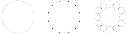
Figure 11. Circle graph, circle with multi vertices and the corresponding double graph.

Lemma 3.10.

Let $\Gamma$ be a graph. The following identities hold:

$$\begin{split}&(i)\qquad R_{i}(\Gamma^{DA,n})=\frac{1}{n}\frac{L_{i}R_{i}}{(nL_{i}+(n-1)R_{i})}.\\ &(ii)\qquad\sum_{e_{i}\in\,E(\Gamma^{DA,n})}\frac{L_{i}(\Gamma^{DA,n})^{2}}{L_{i}(\Gamma^{DA,n})+R_{i}(\Gamma^{DA,n})}=\frac{n-1}{n}\ell(\Gamma)+\frac{1}{n}\sum_{e_{i}\in\,E(\Gamma)}\frac{L_{i}^{2}}{L_{i}+R_{i}}.\end{split}$$

Proof.

The proof of $(i)$: By the proof of Theorem 3.4 with its notation $a$, $b$, $d$,

$$\begin{split}R_{i}(\Gamma^{DA,n})=\frac{d(a+b)}{d+a+b}=\frac{\frac{L_{i}}{n(n-1)}\frac{R_{i}}{n^{2}}}{\frac{L_{i}}{n(n-1)}+\frac{R_{i}}{n^{2}}}=\frac{1}{n}\frac{L_{i}R_{i}}{(nL_{i}+(n-1)R_{i})}.\end{split}$$

The proof of $(ii)$: By using part $(i)$,

$$\begin{split}\sum_{e_{i}\in\,E(\Gamma^{DA,n})}\frac{L_{i}(\Gamma^{DA,n})^{2}}{L_{i}(\Gamma^{DA,n})+R_{i}(\Gamma^{DA,n})}=n\sum_{e_{i}\in\,E(\Gamma)}\frac{(\frac{L_{i}}{n})^{2}}{\frac{L_{i}}{n}+\frac{1}{n}\frac{L_{i}R_{i}}{nL_{i}+(n-1)R_{i}}}.\end{split}$$

Then the result follows. ∎

Theorem 3.11.

Let $\Gamma$ be a graph with $\ell(\Gamma)=1$. Suppose $\tau(\Gamma^{DA,n})\geq\frac{1}{108}\big{(}\frac{3n-2}{n}\big{)}^{2}$. Then $\tau(\Gamma)\geq\frac{1}{108}$.

Proof.

By Theorem 3.4, $\tau(\Gamma)=n^{2}\tau(\Gamma^{DA,n})-\frac{(n-1)^{2}}{12}-\frac{n-1}{6}\sum_{e_{i}\in\,E(\Gamma)}\frac{L_{i}^{2}}{L_{i}+R_{i}}.$ On the other hand, by the proof of Theorem 2.24 $\tau(\Gamma)\geq\frac{1}{12}\Big{(}\sum_{e_{i}\in\,E(\Gamma)}\frac{L_{i}^{2}}{L_{i}+R_{i}}\Big{)}^{2}.$ Let $x=\sum_{e_{i}\in\,E(\Gamma)}\frac{L_{i}^{2}}{L_{i}+R_{i}}$ and $y=\tau(\Gamma)$; then we have

(18) $$y\geq\frac{(3n-2)^{2}}{108}-\frac{(n-1)^{2}}{12}-\frac{n-1}{6}x\quad\text{and }y\geq\frac{x^{2}}{12}.$$

The line and the parabola, obtained by considering inequalities in Equation (18) as equalities, in $xy-$plane intersect at $x=\frac{1}{3}$ and $y=\frac{1}{108}$, since $n\geq 1$. Hence, (18) implies the result. ∎

Corollary 3.12.

Let $\Gamma$ be a graph with $\ell(\Gamma)=1$. If $\tau(\Gamma^{DA})\geq\frac{1}{27}$ or $\tau(\Gamma^{DA,3})\geq\frac{49}{972}$, then $\tau(\Gamma)\geq\frac{1}{108}$.

Proof.

The result follows from Theorem 3.11. ∎

In section §4, we will give far-reaching generalizations of Theorem 3.4 and Theorem 3.8.

4. The tau constant and graph immersions

In this section, we will define another graph operation which will be a generalization of the process of obtaining $\Gamma^{DA,n}$ from a graph $\Gamma$ as presented in §3. Let $r(x,y)$ and $r^{n}(x,y)$ be the resistance functions on $\Gamma$ and $\Gamma^{DA,n}$, respectively. First we reinterpret the way we constructed $\Gamma^{DA,n}$ in order to clarify how to generalize it.

Given a graph $\Gamma$ and a $n$-banana graph $\beta_{n}$ (the graph with $n$ parallel edges of equal length between vertices $p$ and $q$) we replaced each edge of $\Gamma$ by $\beta_{n,i}$, a copy of $\beta_{n}$ scaled so that each edge had length $nL_{i}$. Then, we divided each edge length by $n^{2}$ to have $\ell(\Gamma^{DA,n})=\ell(\Gamma)$. In this operation the following features were important in enabling us to compute $\tau(\Gamma^{DA,n})$ in terms of $\tau(\Gamma)$:

• We started with a graph $\Gamma$ and a graph $\beta_{n}$ with distinguished points $p$ and $q$.

• We replaced each edge $e_{i}$ of $\Gamma$ by $\beta_{n,i}$, a copy of $\beta_{n}$, scaled so that $r_{\beta_{n,i}}(p,q)=L_{i}$.

• After all the edge replacements were done we obtained a graph which had total length $n^{2}\ell(\Gamma)$. We divided each edge length of this graph by $n^{2}$ to obtain $\Gamma^{DA,n}$, so that $\ell(\Gamma^{DA,n})=\ell(\Gamma)$.

• We kept the vertex set of $\Gamma$ in the vertex set of $\Gamma^{DA,n}$, $V(\Gamma)=V(\Gamma^{DA,n})$ and for any $p$, $q$ in $V(\Gamma)$, we had $r^{n}(p,q)=\frac{r(p,q)}{n^{2}}.$

Now consider the following more general setup.

Let $\Gamma$ and $\beta$ be two given graphs with $\ell(\Gamma)=\ell(\beta)=1$. Let $p$ and $q$ be any two distinct points in $\beta$. For every edge $e_{i}\in E(\Gamma)$, if $e_{i}$ has length $L_{i}$, let $\beta_{i}$ be the graph obtained from $\beta$ by multiplying each edge length in $\beta$ by $\frac{L_{i}}{r_{\beta}(p,q)}$ where $r_{\beta}(x,y)$ is the resistance function in $\beta$. Then $\ell(\beta_{i})=\frac{L_{i}}{r_{\beta}(p,q)}$, and if $r_{\beta_{i}}(x,y)$ is the resistance function in $\beta_{i}$, then $r_{\beta_{i}}(p,q)=L_{i}$. For each edge $e_{i}\in E(\Gamma)$, if $e_{i}$ has end points $p_{i}$ and $q_{i}$, we replace $e_{i}$ by $\beta_{i}$, identify $p_{i}$ with $p$ and $q_{i}$ with $q$. (The choice of the labeling of the end points of $e_{i}$ does not change the $\tau$-constant of the graph obtained, as the computations below will show clearly. However, we will assume that a labeling of the end points is given, so that the graph obtained at the end of edge replacements will be uniquely determined.) This gives a new graph which we will denote $\Gamma\star\beta_{p,q}$, and call “the full immersion of $\beta$ into $\Gamma$ with respect to $p$ and $q$” (see Figure 15). Note that

(19) $$\ell(\Gamma\star\beta_{p,q})=\sum_{e_{i}\in E(\Gamma)}\ell(\beta_{i})=\sum_{e_{i}\in E(\Gamma)}\frac{L_{i}}{r_{\beta}(p,q)}=\frac{\ell(\Gamma)}{r_{\beta}(p,q)}=\frac{1}{r_{\beta}(p,q)}.$$

Having constructed $\Gamma\star\beta_{p,q}$, we divide each edge length by $\ell(\Gamma\star\beta_{p,q})$, obtaining the normalized graph $(\Gamma\star\beta_{p,q})^{N}$, with $\ell((\Gamma\star\beta_{p,q})^{N})=1=\ell(\Gamma).$

Our goal in this section is to compute $\tau((\Gamma\star\beta_{p,q})^{N})$. We begin with some preliminary computations which will also be useful in later sections.

Notation.

Define $A_{p,q,\Gamma}:=\int_{\Gamma}j_{x}(p,q)({\frac{d}{dx}}j_{p}(x,q))^{2}dx.$

Note that $A_{p,q,\Gamma}\geq 0$ for any p, q $\in\Gamma$. The importance of $A_{p,q,\Gamma}$ will be clear when we examine its relation to $\tau(\Gamma)$ in later sections. In some sense it is “the” basic hard-to-evaluate graph integral, and many other integrals can be evaluated in terms of it.

Remark 4.1 (Scaling Property for $A_{p,q,\Gamma}$).

Let $\Gamma$ be a graph and let $\beta$ be a graph obtained by multiplying length of each edge in $E(\Gamma)$ by a constant $c$. Then $\ell(\beta)=c\ell(\Gamma)$, $V(\beta)=V(\Gamma)$, $j_{x}^{\beta}(p,q)=cj_{x}(p,q)$, and $A_{p,q,\beta}=c^{2}A_{p,q,\Gamma}$ for any $p$ and $q$ in $V(\Gamma)$.

Remark 4.2.

For any p, q and x $\in\Gamma$, $\frac{d}{dx}j_{p}(x,q)=-\frac{d}{dx}j_{q}(x,p)$, since $r(p,q)=j_{p}(x,q)+j_{q}(x,p)$.

Theorem 4.3.

For any p, q $\in\Gamma$, the following quantities are all equal to each other:

$$(i)\,\,A_{p,q,\Gamma}\quad (ii)\,\,\frac{1}{2}\int_{\Gamma}j_{x}(p,q)\Delta_{x}(j_{p}(x,q)j_{q}(x,p))\quad\quad\quad$$

$$(iii)\,\,\frac{1}{2}\int_{\Gamma}j_{p}(x,q)j_{q}(x,p)\Delta_{x}j_{x}(p,q)\quad (iv)\,\,-\int_{\Gamma}j_{p}(x,q){\frac{d}{dx}}j_{p}(x,q){\frac{d}{dx}}j_{x}(p,q)dx\quad$$

$$(v)\,\,\int_{\Gamma}j_{q}(x,p){\frac{d}{dx}}j_{p}(x,q){\frac{d}{dx}}j_{x}(p,q)dx\quad (vi)\,\,-\frac{r(p,q)^{2}}{2}+\int_{\Gamma}r(p,x)({\frac{d}{dx}}j_{p}(x,q))^{2}dx$$

Proof.

(i) and (ii) are equal:

$$\begin{split}\int_{\Gamma}j_{x}(p,q)&\Delta_{x}(j_{p}(x,q)j_{q}(x,p))=\int_{\Gamma}j_{x}(p,q)\Big{(}j_{q}(x,p)\Delta_{x}j_{p}(x,q)+j_{p}(x,q)\Delta_{x}j_{q}(x,p)\\ &\quad-2{\frac{d}{dx}}j_{p}(x,q){\frac{d}{dx}}j_{q}(x,p)dx\Big{)},\quad\text{by Theorem~{}\ref{thmdelta}};\\ &=\int_{\Gamma}j_{x}(p,q)j_{q}(x,p)(\delta_{q}(x)-\delta_{p}(x))+\int_{\Gamma}j_{x}(p,q)j_{p}(x,q)(\delta_{p}(x)-\delta_{q}(x))\\ &\quad-2\int_{\Gamma}j_{x}(p,q){\frac{d}{dx}}j_{p}(x,q){\frac{d}{dx}}j_{q}(x,p)dx,\quad\text{by Proposition~{}\ref{prop cordjpq}};\\ &=j_{q}(p,q)j_{q}(q,p)-j_{p}(p,q)j_{q}(p,p)+j_{p}(p,q)j_{p}(p,q)-j_{q}(p,q)j_{p}(q,q)\\ &\quad+2\int_{\Gamma}j_{x}(p,q)({\frac{d}{dx}}j_{p}(x,q))^{2}dx,\quad\text{by Remark~{}\ref{remjpq}};\\ &=2\int_{\Gamma}j_{x}(p,q)({\frac{d}{dx}}j_{p}(x,q))^{2}dx,\quad\text{since $j_{q}(p,q)=0=j_{p}(p,q)$};\\ &=2A_{p,q,\Gamma}.\end{split}$$

(ii) and (iii) are equal: This follows from the self-adjointness of $\Delta_{x}$, see Proposition 2.2.
(iii) and (iv) are equal:

$$\begin{split}\frac{1}{2}&\int_{\Gamma}j_{p}(x,q)j_{q}(x,p)\Delta_{x}j_{x}(p,q)=\frac{1}{2}\int_{\Gamma}{\frac{d}{dx}}\big{[}j_{p}(x,q)j_{q}(x,p)\big{]}{\frac{d}{dx}}j_{x}(p,q)dx\\ &=\frac{1}{2}\int_{\Gamma}{\frac{d}{dx}}j_{x}(p,q)\big{[}j_{q}(x,p){\frac{d}{dx}}j_{p}(x,q)-j_{p}(x,q){\frac{d}{dx}}j_{p}(x,q)\big{]}dx,\quad\text{by Remark~{}\ref{remjpq}};\\ &=\frac{1}{2}\int_{\Gamma}{\frac{d}{dx}}j_{x}(p,q){\frac{d}{dx}}j_{p}(x,q)\big{[}r(p,q)-2j_{p}(x,q)\big{]}dx\\ &=\frac{r(p,q)}{2}\int_{\Gamma}{\frac{d}{dx}}j_{x}(p,q){\frac{d}{dx}}j_{p}(x,q)dx-\int_{\Gamma}j_{p}(x,q){\frac{d}{dx}}j_{x}(p,q){\frac{d}{dx}}j_{p}(x,q)dx\\ &=-\int_{\Gamma}j_{p}(x,q){\frac{d}{dx}}j_{p}(x,q){\frac{d}{dx}}j_{x}(p,q)dx,\quad\text{by Lemma~{}\ref{lemorthogonality}}.\end{split}$$

(iv) and (v) are equal:

$$\begin{split}-\int_{\Gamma}&j_{p}(x,q){\frac{d}{dx}}j_{p}(x,q){\frac{d}{dx}}j_{x}(p,q)dx=-\int_{\Gamma}\big{[}r(p,q)-j_{q}(x,p)\big{]}{\frac{d}{dx}}j_{p}(x,q){\frac{d}{dx}}j_{x}(p,q)dx\\ &=-r(p,q)\cdot 0+\int_{\Gamma}j_{q}(x,p){\frac{d}{dx}}j_{p}(x,q){\frac{d}{dx}}j_{x}(p,q)dx,\quad\text{by Lemma~{}\ref{lemorthogonality}}.\end{split}$$

(i) and (vi) are equal: By Equation (2),

$$\begin{split}A_{p,q,\Gamma}=\int_{\Gamma}j_{x}(p,q)({\frac{d}{dx}}j_{p}(x,q))^{2}dx=\int_{\Gamma}(r(p,x)-j_{p}(x,q))({\frac{d}{dx}}j_{p}(x,q))^{2}dx.\end{split}$$

Hence the result follows from Corollary 2.19. ∎

Example 4.4.

Let $\Gamma$ be the graph, which we will call the “diamond graph”, shown in Figure 12. Assume the edges $\{e_{1},\,\dots,e_{5}\}$ and the vertices $\{a,\,b,\,p,\,q\}$ are labeled as shown. Let each edge length be $L$. By the symmetry of the graph, edges $e_{1}$, $e_{2}$, $e_{3}$ and $e_{4}$ make the same contribution to $A_{p,q,\Gamma}$. After circuit reductions and computations in Maple, we obtain that $j_{p}(x,q)$ is constant on $e_{5}$, where $j_{x}(y,z)$ is the voltage function in $\Gamma$. (Alternatively, $j_{p}(a,q)=j_{p}(b,q)$ by the symmetry again, so $j_{p}(x,q)$ must be constant on $e_{5}$.) Therefore,

$$A_{p,q,\Gamma}=\int_{\Gamma}j_{x}(p,q)({\frac{d}{dx}}j_{p}(x,q))^{2}dx=4\int_{e_{1}}j_{x}(p,q)({\frac{d}{dx}}j_{p}(x,q))^{2}dx.$$

Using circuit reductions and computations in Maple, one finds ${\frac{d}{dx}}j_{p}(x,q)=\frac{1}{2}$ and $j_{x}(p,q)=\frac{x(4L-3x)}{8L}$. Evaluating the integral gives $A_{p,q,\Gamma}=\frac{L^{2}}{8}$.

Figure 12. Diamond graph.

Proposition 4.5.

Let $\Gamma$ be a tree. Then, for any points $p$ and $q$ in $\Gamma$, $A_{p,q,\Gamma}=0$.

Proof.

Let $j_{x}(y,z)$ be the voltage function in $\Gamma$. Let $e_{i}\in E(\Gamma)$. If $e_{i}$ is not between $p$ and $q$, then ${\frac{d}{dx}}j_{p}(x,q)=0$ for all $x\in e_{i}$. If $e_{i}$ is between $p$ and $q$, then $j_{x}(p,q)=0$ for all $x\in e_{i}$. Therefore, $j_{x}(p,q)({\frac{d}{dx}}j_{p}(x,q))^{2}=0$ for every $x\in\Gamma$. This gives, by definition, $A_{p,q,\Gamma}=0.$ ∎

The following proposition is similar to the additive property of $\tau$.

Proposition 4.6 (Additive Property for $A_{p,q,\Gamma}$).

Let $\Gamma$, $\Gamma_{1}$ and $\Gamma_{2}$ be graphs such that $\Gamma=\Gamma_{1}\cup\Gamma_{2}$ and $\Gamma_{1}\cap\Gamma_{2}=\{y\}$ for some $y\in\Gamma$. For any $p\in\Gamma_{1}$ and $q\in\Gamma_{2}$,

$$A_{p,q,\Gamma}=A_{p,y,\Gamma_{1}}+A_{y,q,\Gamma_{2}}.$$

Proof.

Let $j_{x}(p,q)$, $j_{x}^{1}(p,q)$ and $j_{x}^{2}(p,q)$ be the voltage functions in $\Gamma$, $\Gamma_{1}$ and $\Gamma_{2}$ respectively. For any $x\in\Gamma_{1}$, after circuit reduction, we obtain the first graph in Figure 13. Note that $s$ is independent of $x$, so ${\frac{d}{dx}}(s)=0.$ Also, $j_{x}(p,q)=j_{x}^{1}(p,y)$.

Similarly, after circuit reduction, for any $x\in\Gamma_{2}$ we obtain the second graph in Figure 13. Note that $S$ is independent of $x$, so ${\frac{d}{dx}}S=0.$ Also, $j_{x}(p,q)=j_{x}^{2}(p,y)$.

Figure 13. Circuit reductions for $\Gamma=\Gamma_{1}\cup\Gamma_{2}$.

Thus

$$\begin{split}A_{p,q,\Gamma}&=\int_{\Gamma}j_{x}(p,q)({\frac{d}{dx}}j_{p}(x,q))^{2}dx\\ &=\int_{\Gamma_{1}}j_{x}^{1}(p,q)({\frac{d}{dx}}j_{p}^{1}(x,q))^{2}dx+\int_{\Gamma_{2}}j_{x}^{2}(p,q)({\frac{d}{dx}}j^{2}_{p}(x,q))^{2}dx.\end{split}$$

Then the result follows from the definitions of $A_{p,y,\Gamma_{1}}$ and $A_{y,q,\Gamma_{2}}$. ∎

The following theorem gives value of $\tau((\Gamma\star\beta_{p,q})^{N})$ in terms of $\tau(\Gamma)$, $\tau(\beta)$, $r_{\beta}(p,q)$ and two other constants related to $\Gamma$ and $\beta$.

Theorem 4.7.

Let $\Gamma$ and $\beta$ be two graphs with $\ell(\Gamma)=\ell(\beta)=1$, and let $p$ and $q$ be two distinct points in $V(\beta)$. Let $r_{\beta}(x,y)$ be the resistance function on $\beta$. Then,

$$\tau((\Gamma\star\beta_{p,q})^{N})=\tau(\beta)-\frac{r_{\beta}(p,q)}{4}+r_{\beta}(p,q)\tau(\Gamma)+\frac{A_{p,q,\beta}}{r_{\beta}(p,q)}\sum_{e_{i}\in E(\Gamma)}\frac{L_{i}^{2}}{L_{i}+R_{i}}.$$

Proof.

We will first compute $\tau(\Gamma\star\beta_{p,q})$. Let $y$ be a fixed point in the vertex set $V(\Gamma)$ and let $r(x,y)$ be the resistance function in $\Gamma\star\beta_{p,q}$. Then, by Corollary 2.4,

(20) $$\begin{split}\tau(\Gamma\star\beta_{p,q})&=\frac{1}{4}\int_{\Gamma\star\beta_{p,q}}\big{(}{\frac{d}{dx}}r(x,y)\big{)}^{2}dx=\frac{1}{4}\sum_{e_{i}\in E(\Gamma)}\int_{\beta_{i}}\big{(}{\frac{d}{dx}}r(x,y)\big{)}^{2}dx.\end{split}$$

Figure 14. Circuit reduction for $\Gamma\star\beta_{p,q}$ with reference to $p$, $q$, $y$, and $x$.

Consider a point $x\in\beta_{i}$. By carrying out circuit reductions in $\beta_{i}$ and in $\Gamma-e_{i}$, we obtain a network with equivalent resistance between the points $x$, $p$, $q$, $y$ as shown in Figure 14. Note that in this new circuit, the existence of the part with edges $d$, $f$ and $h$ depends on the fact that $y$, being a point in $V(\Gamma)$, belongs to $\Gamma-e_{i}$. It is possible that $y=p$ or $y=q$, in which cases some of the edge lengths in $\{d,\,f,\,h\}$ are $0$. It is also possible that $\Gamma-e_{i}$ is disconnected, in which case $d$ or $f$ will be $\infty$. Let $j^{\beta_{i}}_{x}(y,z)$ be the voltage function in $\beta_{i}$ and $R_{a_{i},y}$, $R_{b_{i},y}$, $R_{c_{i},y}$ be the voltages in $\Gamma-e_{i}$, using the same notation as in Proposition 2.9. Then the resistances in Figure 14 are as follows: $a={j^{\beta_{i}}_{x}(p,q)}$, $b={j^{\beta_{i}}_{p}(x,q)}$, $c={j^{\beta_{i}}_{q}(x,p)}$, $f=R_{a_{i},y}$, $d=R_{b_{i},y}$, $h=R_{c_{i},y}$. Note that the values in the figure are results of our conditions on $\beta_{i}$ and the replacements that are made. Note also that $b+c=r_{\beta_{i}}(p,q)=L_{i}$ and $f+d=R_{i}$, so as $x$ varies along an edge of $\beta_{i}$, we have ${\frac{d}{dx}}b=-{\frac{d}{dx}}c$. Since $r_{\beta_{j}}(p,q)=L_{j}$ for each $e_{j}\in E(\Gamma-e_{j})$, $\Gamma\star\beta_{p,q}$ can be transformed to the circuit in 14.

By applying parallel reduction,

$$\begin{split}r(x,y)=a+\frac{(b+f)(c+d)}{b+c+d+f}+h={j^{\beta_{i}}_{x}(p,q)}+\frac{({j^{\beta_{i}}_{p}(x,q)}+R_{a_{i},y})({j^{\beta_{i}}_{q}(x,p)}+R_{b_{i},y})}{L_{i}+R_{i}}+R_{c_{i},p}.\end{split}$$

Therefore,

$$\begin{split}{\frac{d}{dx}}r(x,y)={\frac{d}{dx}}{j^{\beta_{i}}_{x}(p,q)}+\frac{{j^{\beta_{i}}_{q}(x,p)}+R_{b_{i},y}}{L_{i}+R_{i}}{\frac{d}{dx}}{j^{\beta_{i}}_{p}(x,q)}+\frac{{j^{\beta_{i}}_{p}(x,q)}+R_{a_{i},y}}{L_{i}+R_{i}}{\frac{d}{dx}}{j^{\beta_{i}}_{q}(x,p)}.\end{split}$$

Since $\,{\frac{d}{dx}}{j^{\beta_{i}}_{q}(x,p)}=-{\frac{d}{dx}}{j^{\beta_{i}}_{p}(x,q)}$ and ${j^{\beta_{i}}_{p}(x,q)}+{j^{\beta_{i}}_{q}(x,p)}=L_{i}$,

$$\begin{split}{\frac{d}{dx}}r(x,y)&={\frac{d}{dx}}{j^{\beta_{i}}_{x}(p,q)}+\frac{L_{i}-2{j^{\beta_{i}}_{p}(x,q)}+R_{b_{i},y}-R_{a_{i},y}}{L_{i}+R_{i}}{\frac{d}{dx}}{j^{\beta_{i}}_{p}(x,q)}.\end{split}$$

Thus,

(21) $$\begin{split}&\int_{\beta_{i}}\big{(}{\frac{d}{dx}}r(x,y)\big{)}^{2}dx=\int_{\beta_{i}}\big{(}{\frac{d}{dx}}{j^{\beta_{i}}_{x}(p,q)}\big{)}^{2}dx+\Big{[}\frac{L_{i}+R_{b_{i},y}-R_{a_{i},y}}{L_{i}+R_{i}}\Big{]}^{2}\int_{\beta_{i}}\big{(}{\frac{d}{dx}}{j^{\beta_{i}}_{p}(x,q)}\big{)}^{2}dx\\ &\qquad+\frac{4}{(L_{i}+R_{i})^{2}}\int_{\beta_{i}}\big{[}{j^{\beta_{i}}_{p}(x,q)}{\frac{d}{dx}}{j^{\beta_{i}}_{p}(x,q)}\big{]}^{2}dx\\ &\qquad+2\Big{[}\frac{L_{i}+R_{b_{i},y}-R_{a_{i},y}}{L_{i}+R_{i}}\Big{]}\int_{\beta_{i}}{\frac{d}{dx}}{j^{\beta_{i}}_{x}(p,q)}{\frac{d}{dx}}{j^{\beta_{i}}_{p}(x,q)}dx\\ &\qquad-\frac{4}{L_{i}+R_{i}}\int_{\beta_{i}}{j^{\beta_{i}}_{p}(x,q)}{\frac{d}{dx}}{j^{\beta_{i}}_{p}(x,q)}{\frac{d}{dx}}{j^{\beta_{i}}_{x}(p,q)}dx\\ &\qquad-4\frac{L_{i}+R_{b_{i},y}-R_{a_{i},y}}{(L_{i}+R_{i})^{2}}\int_{\beta_{i}}{j^{\beta_{i}}_{p}(x,q)}\big{[}{\frac{d}{dx}}{j^{\beta_{i}}_{p}(x,q)}\big{]}^{2}dx.\end{split}$$

On the other hand, we have

(22) $$\begin{split}&\text{By Corollary~{}\ref{corjrpq}, }\quad\int_{\beta_{i}}\big{(}{\frac{d}{dx}}{j^{\beta_{i}}_{p}(x,q)}\big{)}^{2}dx=r_{\beta_{i}}(p,q).\\ &\text{By Corollary~{}\ref{corjrpq}, }\quad\int_{\beta_{i}}\big{[}{j^{\beta_{i}}_{p}(x,q)}{\frac{d}{dx}}{j^{\beta_{i}}_{p}(x,q)}\big{]}^{2}dx=\frac{1}{3}(r_{\beta_{i}}(p,q))^{3}.\\ &\text{By Lemma~{}\ref{lemorthogonality}, }\quad\int_{\beta_{i}}{\frac{d}{dx}}{j^{\beta_{i}}_{x}(p,q)}{\frac{d}{dx}}{j^{\beta_{i}}_{p}(x,q)}dx=0.\\ &\text{By Theorem~{}\ref{thmremain}, }\quad\int_{\beta_{i}}{j^{\beta_{i}}_{p}(x,q)}{\frac{d}{dx}}{j^{\beta_{i}}_{x}(p,q)}{\frac{d}{dx}}{j^{\beta_{i}}_{p}(x,q)}dx=-A_{p,q,\beta_{i}}.\\ &\text{By Corollary~{}\ref{corjrpq}, }\quad\int_{\beta_{i}}{j^{\beta_{i}}_{p}(x,q)}\big{[}{\frac{d}{dx}}{j^{\beta_{i}}_{p}(x,q)}\big{]}^{2}dx=\frac{1}{2}(r_{\beta_{i}}(p,q))^{2}.\end{split}$$

Substituting the results in Equation (22) into Equation (21), and recalling $r_{\beta_{i}}(p,q)=L_{i}$, gives

(23) $$\begin{split}\int_{\beta_{i}}\big{(}{\frac{d}{dx}}r(x,y)\big{)}^{2}dx&=\int_{\beta_{i}}\big{(}{\frac{d}{dx}}{j^{\beta_{i}}_{x}(p,q)}\big{)}^{2}dx+\Big{[}\frac{L_{i}+R_{b_{i},y}-R_{a_{i},y}}{L_{i}+R_{i}}\Big{]}^{2}L_{i}\\ &\qquad+\frac{4L_{i}^{3}}{3(L_{i}+R_{i})^{2}}+\frac{4A_{p,q,\beta_{i}}}{L_{i}+R_{i}}-4\frac{L_{i}+R_{b_{i},y}-R_{a_{i},y}}{(L_{i}+R_{i})^{2}}\frac{L_{i}^{2}}{2}\\ &=\int_{\beta_{i}}\big{(}{\frac{d}{dx}}{j^{\beta_{i}}_{x}(p,q)}\big{)}^{2}dx+\frac{L_{i}^{3}+3L_{i}(R_{b_{i},y}-R_{a_{i},y})^{2}}{3(L_{i}+R_{i})^{2}}+\frac{4A_{p,q,\beta_{i}}}{L_{i}+R_{i}}.\end{split}$$

By applying Theorem 2.21 to $\beta_{i}$, we obtain

$$\int_{\beta_{i}}\big{(}{\frac{d}{dx}}{j^{\beta_{i}}_{x}(p,q)}\big{)}^{2}dx=4\tau(\beta_{i})-r_{\beta_{i}}(p,q)=4\tau(\beta_{i})-L_{i}.$$

Substituting this into Equation (23) and summing up over all edges in $E(\Gamma)$ gives

(24) $$\begin{split}\sum_{e_{i}\in E(\Gamma)}\int_{\beta_{i}}\big{(}{\frac{d}{dx}}r(x,y)\big{)}^{2}dx&=4\sum_{e_{i}\in E(\Gamma)}\tau(\beta_{i})-\sum_{e_{i}\in E(\Gamma)}L_{i}+4\sum_{e_{i}\in E(\Gamma)}\frac{A_{p,q,\beta_{i}}}{L_{i}+R_{i}}\\ &\qquad+\frac{1}{3}\sum_{e_{i}\in E(\Gamma)}\frac{L_{i}^{3}+3L_{i}(R_{b_{i},y}-R_{a_{i},y})^{2}}{(L_{i}+R_{i})^{2}}\\ &=4\sum_{e_{i}\in E(\Gamma)}\tau(\beta_{i})\,-1+4\sum_{e_{i}\in E(\Gamma)}\frac{A_{p,q,\beta_{i}}}{L_{i}+R_{i}}+4\tau(\Gamma).\end{split}$$

The second equality in Equation (24) follows from Proposition 2.9. By using Remarks (2.15) and (4.1) and the fact that $\ell(\beta_{i})=\frac{L_{i}}{r_{\beta}(p,q)}$, we obtain

(25) $$\begin{split}&\tau(\beta_{i})=\frac{L_{i}}{r_{\beta}(p,q)}\tau(\beta),\quad\text{and }A_{p,q,\beta_{i}}=\Big{[}\frac{L_{i}}{r_{\beta}(p,q)}\Big{]}^{2}A_{p,q,\beta}.\end{split}$$

Substituting the results in Equation (25) into Equation (24) gives

(26) $$\begin{split}\sum_{e_{i}\in E(\Gamma)}\int_{\beta_{i}}\big{(}{\frac{d}{dx}}r(x,y)\big{)}^{2}dx=4\frac{\tau(\beta)}{r_{\beta}(p,q)}\sum_{e_{i}\in E(\Gamma)}L_{i}+4\tau(\Gamma)-1+\frac{4A_{p,q,\beta}}{(r_{\beta}(p,q))^{2}}\sum_{e_{i}\in E(\Gamma)}\frac{L_{i}^{2}}{L_{i}+R_{i}}.\end{split}$$

Substituting Equation (26) into Equation (20) gives

(27) $$\begin{split}\tau(\Gamma\star\beta_{p,q})&=\frac{\tau(\beta)}{r_{\beta}(p,q)}+\tau(\Gamma)-\frac{1}{4}+\frac{A_{p,q,\beta}}{(r_{\beta}(p,q))^{2}}\sum_{e_{i}\in E(\Gamma)}\frac{L_{i}^{2}}{L_{i}+R_{i}}.\end{split}$$

Since $\ell(\Gamma\star\beta_{p,q})=\frac{1}{r_{\beta}(p,q)}$ by Equation (19), for the normalized graph $(\Gamma\star\beta_{p,q})^{N}$ we have

$$\tau((\Gamma\star\beta_{p,q})^{N})=\tau(\beta)+r_{\beta}(p,q)\tau(\Gamma)-\frac{r_{\beta}(p,q)}{4}+\frac{A_{p,q,\beta}}{r_{\beta}(p,q)}\sum_{e_{i}\in E(\Gamma)}\frac{L_{i}^{2}}{L_{i}+R_{i}}.$$

This is what we want to show. ∎

Theorem 4.8.

Let $\Gamma$ be a normalized graph. Let $r(x,y)$ be the resistance function on $\Gamma$, and let $p$ and $q$ be any two points in $\Gamma$. Then for any $\varepsilon>0$, there exists a normalized graph $\Gamma^{\prime}$ such that

$$\tau(\Gamma^{\prime})\leq\tau(\Gamma)-r(p,q)(\frac{1}{4}-\tau(\Gamma))+\varepsilon.$$

In particular, if Conjecture  2.13 holds with a constant $C$, then there is no normalized graph $\beta$ with $\tau(\beta)=C$.

Proof.

Let $\Gamma^{m}$ be the graph defined in §3. Then by Lemma 3.7,

(28) $$\begin{split}\sum_{e_{k}\in E(\Gamma^{m})}\frac{L_{k}(\Gamma^{m})^{2}}{L_{k}(\Gamma^{m})+R_{k}(\Gamma^{m})}=\frac{1}{m}\sum_{e_{i}\in E(\Gamma)}\frac{L_{i}^{2}}{L_{i}+R_{i}}.\end{split}$$

Fix distinct points $p$, $q$ in $\Gamma$. Equation (28) and Theorem 4.7 applied to $\Gamma^{m}$ and $\Gamma$ give

(29) $$\begin{split}\tau((\Gamma^{m}\star\Gamma_{p,q})^{N})=\tau(\Gamma)-r(p,q)(\frac{1}{4}-\tau(\Gamma))+\frac{A_{p,q,\Gamma}}{m\cdot r(p,q)}\sum_{e_{i}\in E(\Gamma)}\frac{L_{i}^{2}}{L_{i}+R_{i}}.\end{split}$$

Since $\displaystyle\frac{A_{p,q,\Gamma}}{r(p,q)}\sum_{e_{i}\in E(\Gamma)}\frac{L_{i}^{2}}{L_{i}+R_{i}}$ is independent of $m$, we can choose $m$ large enough to make $\displaystyle\frac{A_{p,q,\Gamma}}{m\cdot r(p,q)}\sum_{e_{i}\in E(\Gamma)}\frac{L_{i}^{2}}{L_{i}+R_{i}}\leq\varepsilon$ for any given $\varepsilon>0$. Then taking $\Gamma^{\prime}:=(\Gamma^{m}\star\Gamma_{p,q})^{N}$ gives the inequality we wanted to show.

Suppose Conjecture  2.13 holds with a constant $C$ and that $\beta$ is a normalized graph with $\tau(\beta)=C$. Then we have $\tau(\beta)\leq\frac{1}{12}$ since $\tau(\Gamma)=\frac{1}{12}$ for the normalized circle graph $\Gamma$ by Corollary 2.17. Thus, $\frac{1}{4}-\tau(\beta)>0$. Let $p$ and $q$ be distinct points in $\beta$, and let $\beta^{\prime}:=(\beta^{m}\star\beta_{p,q})^{N}$. For sufficiently large $m$, we have $\tau(\beta^{\prime})<\tau(\beta)$ by the inequality we proved. This contradicts with the assumption made for $\beta$. This completes the proof of the theorem. ∎

The proof of Theorem 4.7 suggests a further generalization of Theorem 4.7, as follows:

Let $\Gamma$ be a graph with $\ell(\Gamma)=1$ and $e$ edges. For each $i=1,2,\dots,e$, suppose $\beta^{i}$ is a graph with $\ell(\beta^{i})=1$. Let $p_{i}$ and $q_{i}$ be any two distinct points in $V(\beta^{i})$, and let $r_{\beta^{i}}(x,y)$ be the resistance function in $\beta^{i}$. By multiplying each edge length of $\beta^{i}$ by $\frac{L_{i}}{r_{\beta^{i}}(p_{i},q_{i})}$ we obtain a graph which will be denoted by $\beta_{i}$. Note that $\ell(\beta_{i})=\frac{L_{i}}{r_{\beta^{i}}(p_{i},q_{i})}$ and $r_{\beta_{i}}(p_{i},q_{i})=L_{i}$, where $r_{\beta_{i}}(x,y)$ is the resistance function in $\beta_{i}$. We replace each edge of $\Gamma$ with $\beta_{i}$ and identify the end points of $e_{i}\in E(\Gamma)$ with the points $p_{i}$ and $q_{i}$ in $\beta_{i}$ so that the resistances between points in $V(\Gamma)$ do not change after the replacement. When edge replacements are complete, we obtain a graph which we will denote by $\Gamma\star(\beta^{1}_{p_{1},q_{1}}\times\beta^{2}_{p_{2},q_{2}}\times\dots\times\beta^{e}_{p_{e},q_{e}})$ or by $\Gamma\star\prod_{i=1}^{e}\beta^{i}_{p_{i},q_{i}}$ for short (see Figure 16). Clearly,

(30) $$\ell(\Gamma\star\prod_{i=1}^{e}\beta^{i}_{p_{i},q_{i}})=\sum_{e_{i}\in E(\Gamma)}\ell(\beta_{i})=\sum_{e_{i}\in E(\Gamma)}\frac{L_{i}}{r_{\beta^{i}}(p_{i},q_{i})}.$$

(31) $$\begin{split}\tau(\beta_{i})=\frac{L_{i}}{r_{\beta^{i}}(p_{i},q_{i})}\tau(\beta^{i})\quad\text{and }A_{p_{i},q_{i},\beta_{i}}=\Big{(}\frac{L_{i}}{r_{\beta^{i}}(p_{i},q_{i})}\Big{)}^{2}A_{p_{i},q_{i},\beta^{i}}.\end{split}$$

Let $r(x,y)$ be the resistance function in $\Gamma$. For any fixed $y\in V(\Gamma)$, we can employ the same arguments as in the proof of Theorem 4.7. Therefore, Equation (24) gives

(32) $$\begin{split}\sum_{e_{i}\in E(\Gamma)}\int_{\beta_{i}}\big{(}{\frac{d}{dx}}r(x,y)\big{)}^{2}dx=-1+4\sum_{e_{i}\in E(\Gamma)}\tau(\beta_{i})+4\sum_{e_{i}\in E(\Gamma)}\frac{A_{p_{i},q_{i},\beta_{i}}}{L_{i}+R_{i}}+4\tau(\Gamma).\end{split}$$

Substituting Equations (31) into Equation (32) gives

(33) $$\begin{split}\sum_{e_{i}\in E(\Gamma)}\int_{\beta_{i}}\big{(}{\frac{d}{dx}}r(x,y)\big{)}^{2}dx&=4\tau(\Gamma)-1+\sum_{e_{i}\in E(\Gamma)}\Big{(}\frac{4L_{i}\tau(\beta^{i})}{r_{\beta^{i}}(p_{i},q_{i})}+\frac{4L_{i}^{2}A_{p_{i},q_{i},\beta^{i}}}{(L_{i}+R_{i})(r_{\beta^{i}}(p_{i},q_{i}))^{2}}\Big{)}.\end{split}$$

Using Equation (20) and Equation (33) gives

(34) $$\begin{split}\tau(\Gamma\star\prod_{i=1}^{e}\beta^{i}_{p_{i},q_{i}})=\tau(\Gamma)-\frac{1}{4}+\sum_{e_{i}\in E(\Gamma)}\frac{L_{i}}{r_{\beta^{i}}(p_{i},q_{i})}\tau(\beta^{i})+\sum_{e_{i}\in E(\Gamma)}\frac{L_{i}^{2}A_{p_{i},q_{i},\beta^{i}}}{(L_{i}+R_{i})(r_{\beta^{i}}(p_{i},q_{i}))^{2}}.\end{split}$$

By using Equation (30), we can normalize $\displaystyle\Gamma\star\prod_{i=1}^{e}\beta^{i}_{p_{i},q_{i}}$. In this way, we obtain the following theorem.

Theorem 4.9.

Suppose $\Gamma$ is a normalized metrized graph with $\#(E(\Gamma))=e$. Let $\beta^{i}$ be a normalized metrized graph, and let $p_{i}$ and $q_{i}$ be any two points in $E(\beta^{i})$ for each $i=1,2,\dots,e$. Then

$$\begin{split}\tau(\big{(}\Gamma\star&\prod_{i=1}^{e}\beta^{i}_{p_{i},q_{i}}\big{)}^{N})\sum_{e_{i}\in E(\Gamma)}\frac{L_{i}}{r_{\beta^{i}}(p_{i},q_{i})}=\tau(\Gamma)-\frac{1}{4}+\sum_{e_{i}\in E(\Gamma)}\Big{[}\frac{L_{i}\tau(\beta^{i})}{r_{\beta^{i}}(p_{i},q_{i})}+\frac{L_{i}^{2}A_{p_{i},q_{i},\beta^{i}}}{(L_{i}+R_{i})(r_{\beta^{i}}(p_{i},q_{i}))^{2}}\Big{]}.\end{split}$$

Corollary 4.10.

Let $\Gamma$ and $\beta^{1},\dots,\beta^{e}$ be as before. For each $\,i\in\{1,2,\dots,e\}$, if there exist points $p_{i}$ and $q_{i}$ in $\beta^{i}$ such that $r_{\beta_{i}}(p_{i},q_{i})=r$, where $r_{\beta_{i}}(x,y)$ is the resistance function in $\beta^{i}$, then

$$\tau(\big{(}\Gamma\star\prod_{i=1}^{e}\beta^{i}_{p_{i},q_{i}}\big{)}^{N})=r\cdot\tau(\Gamma)-\frac{r}{4}+\sum_{e_{i}\in E(\Gamma)}L_{i}\tau(\beta^{i})+\frac{1}{r}\sum_{e_{i}\in E(\Gamma)}\frac{L_{i}^{2}}{L_{i}+R_{i}}A_{p_{i},q_{i},\beta^{i}}.$$

Proof.

Setting $r_{\beta_{i}}(p_{i},q_{i})=r$ in Theorem 4.9 gives the result. ∎

Corollary 4.11.

Let $\Gamma$ and $\beta$ be two normalized graphs and let $\#(E(\Gamma))=e$. Let $r_{\beta}(x,y)$ be the resistance function in $\beta$. For any pairs of points $\{p_{1},q_{1}\},\{p_{2},q_{2}\},\dots,\{p_{e},q_{e}\}$ in $\beta$,

$$\begin{split}\tau(\big{(}\Gamma\star\prod_{i=1}^{e}\beta_{p_{i},q_{i}}\big{)}^{N})=\tau(\beta)+\frac{1}{\sum_{e_{i}\in E(\Gamma)}\frac{L_{i}}{r_{\beta}(p_{i},q_{i})}}\Bigg{[}\tau(\Gamma)-\frac{1}{4}+\sum_{e_{i}\in E(\Gamma)}\frac{L_{i}^{2}A_{p_{i},q_{i},\beta}}{(L_{i}+R_{i})(r_{\beta}(p_{i},q_{i}))^{2}}\Bigg{]}.\end{split}$$

Proof.

Setting $\beta^{i}=\beta$ in Theorem 4.9 gives the result. ∎

Figure 15. $\Gamma$, $\beta$ and $\Gamma\star\prod_{i=1}^{e}\beta_{p_{i},q_{i}}$.

Figure 16. $\Gamma$ (edges are numbered), $\beta^{i}$ ($i=1,\cdots,6$) with corresponding $p$ and $q$, and $\Gamma\star\prod_{i=1}^{e}\beta^{i}_{p_{i},q_{i}}$.

5. The tau constant of the union of two graphs along two points

Let $\Gamma_{1}\cup\Gamma_{2}$ denote the union, along two points p and q, of two connected graphs $\Gamma_{1}$ and $\Gamma_{2}$, so that $\Gamma_{1}\cap\Gamma_{2}=\{p,q\}$. Let $r(x,y)$, $r_{1}(x,y)$ and $r_{2}(x,y)$ denote the resistance functions on $\Gamma_{1}\cup\Gamma_{2}$, $\Gamma_{1}$ and $\Gamma_{2}$, respectively. Note that $\ell(\Gamma_{1}\cup\Gamma_{2})=\ell(\Gamma_{1})+\ell(\Gamma_{2})$.

Theorem 5.1.

Let p, q, $r_{1}(p,q)$, $r_{2}(p,q)$, $\Gamma_{1}$, $\Gamma_{2}$ and $\tau(\Gamma_{1}\cup\Gamma_{2})$ be as above. Then,

$$\begin{split}\tau(\Gamma_{1}\cup\Gamma_{2})=\tau(\Gamma_{1})+\tau(\Gamma_{2})-\frac{r_{1}(p,q)+r_{2}(p,q)}{6}+\frac{A_{p,q,\Gamma_{1}}+A_{p,q,\Gamma_{2}}}{r_{1}(p,q)+r_{2}(p,q)}.\end{split}$$

Proof.

Let $\Gamma$ be the circle graph with vertex set $\{p,q\}$, and with edge lengths $L_{1}=\frac{r_{1}(p,q)}{r_{1}(p,q)+r_{2}(p,q)}$ and $L_{2}=\frac{r_{2}(p,q)}{r_{1}(p,q)+r_{2}(p,q)}$. Let $\beta^{1}=\Gamma_{1}^{N}$ and $\beta^{2}=\Gamma_{2}^{N}$. Then the result follows by computing $\tau(\big{(}\Gamma\star\prod_{i=1}^{2}\beta^{i}_{p,q}\big{)}^{N})$, applying Theorem 4.9. ∎

A different proof of Theorem 5.1 can be found in [C1, page 96].

Corollary 5.2.

Suppose $\Gamma:=\Gamma_{1}=\Gamma_{2}$ in Theorem 5.1. Then, $r_{1}(x,y)=r_{2}(x,y)$ and

$$\begin{split}\tau(\Gamma\cup\Gamma)=2\tau(\Gamma)-\frac{r_{1}(p,q)}{3}+\frac{A_{p,q,\Gamma}}{r_{1}(p,q)}.\end{split}$$

Proof.

Since $\Gamma:=\Gamma_{1}=\Gamma_{2}$, clearly, we have $r_{1}(x,y)=r_{2}(x,y)$, $\tau(\Gamma)=\tau(\Gamma_{1})=\tau(\Gamma_{2})$ and $A_{p,q,\Gamma}=A_{p,q,\Gamma_{1}}=A_{p,q,\Gamma_{2}}$. ∎

The following corollary of Theorem 5.1 shows how the tau constant changes by deletion of an edge when the remaining graph is connected.

Corollary 5.3.

Suppose that $\Gamma$ is a graph such that $\Gamma-e_{i}$ is connected, where $e_{i}\in E(\Gamma)$ is an edge with length $L_{i}$ and end points $p_{i}$ and $q_{i}$. Then,

$$\begin{split}\tau(\Gamma)=\tau(\Gamma-e_{i})+\frac{L_{i}}{12}-\frac{R_{i}}{6}+\frac{A_{p_{i},q_{i},\Gamma-e_{i}}}{L_{i}+R_{i}}.\end{split}$$

Proof.

Let $\Gamma_{1}:=e_{i}$ and $\Gamma_{2}:=\Gamma-e_{i}$. Therefore, $\tau(\Gamma_{1})=\frac{L_{i}}{4}$ by Corollary 2.22, $r_{1}(p_{i},q_{i})=L_{i}$, $r_{2}(p_{i},q_{i})=R_{i}$, and $A_{p_{i},q_{i},\Gamma_{1}}=0$ by Proposition 4.5. Then by Theorem 5.1, we have $\tau(\Gamma)=\tau(\Gamma-e_{i})+\frac{L_{i}}{4}-\frac{1}{6}(L_{i}+R_{i})+\frac{A_{p_{i},q_{i},\Gamma-e_{i}}}{L_{i}+R_{i}}$. This gives the result. ∎

Corollary 5.4.

Suppose that $\Gamma$ is a graph such that $\Gamma-e_{i}$, for some edge $e_{i}\in E(\Gamma)$ with length $L_{i}$ and end points $p_{i}$ and $q_{i}$, is connected. For the voltage function $j^{i}_{x}(y,z)$ in $\Gamma-e_{i}$,

$$\begin{split}\tau(\Gamma)=\frac{1}{4}\int_{\Gamma-e_{i}}({\frac{d}{dx}}j^{i}_{x}(p_{i},q_{i}))^{2}dx+\frac{L_{i}+R_{i}}{12}+\frac{A_{p_{i},q_{i},\Gamma-e_{i}}}{L_{i}+R_{i}}.\end{split}$$

Proof.

By Theorem 2.21, $\tau(\Gamma-e_{i})=\frac{1}{4}\int_{\Gamma-e_{i}}({\frac{d}{dx}}j^{i}_{x}(p_{i},q_{i}))^{2}dx+\frac{R_{i}}{4}$. Substituting this into the formula of Corollary 5.3, one obtains the result. ∎

Note that Corollary 5.4 shows that the tau constant $\tau(\Gamma)$ approaches $\frac{\ell(\Gamma)}{12}$ (the tau constant of a circle graph) as we increase one of the edge lengths and fix the other edge lengths.

One wonders how $\tau(\Gamma)$ changes if one changes the length of an edge in the graph $\Gamma$. Lemma 5.5 below sheds some light on the answer:

Lemma 5.5.

Let $\Gamma$ and $\Gamma^{\prime}$ be two graphs such that $\Gamma-e_{i}$ $\Gamma^{\prime}-e_{i}^{\prime}$ are connected, where $e_{i}\in E(\Gamma)$ is of length $L_{i}$ and has end points $p_{i}$, $q_{i}$ and $e_{i}^{\prime}\in E(\Gamma^{\prime})$ is of length $L_{i}+x_{i}$ and has end points $p_{i}$, $q_{i}$. Here, $x_{i}\in{\mathbb{R}}$ is such that $L_{i}+x_{i}\geq 0$. Suppose that $\Gamma-e_{i}$ and $\Gamma^{\prime}-e_{i}^{\prime}$ are copies of each other. Then,

$$\begin{split}\tau(\Gamma^{\prime})=\tau(\Gamma)+\frac{x_{i}}{12}-\frac{x_{i}A_{p_{i},q_{i},\Gamma-e_{i}}}{(L_{i}+R_{i})(L_{i}+R_{i}+x_{i})}.\end{split}$$

Proof.

By Corollary 5.3, $\tau(\Gamma)=\tau(\Gamma-e_{i})+\frac{L_{i}}{12}-\frac{R_{i}}{6}+\frac{A_{p_{i},q_{i},\Gamma-e_{i}}}{L_{i}+R_{i}}.$ Again, by Corollary 5.3 and the fact that $\Gamma-e_{i}=\Gamma^{\prime}-e_{i}^{\prime}$, $\tau(\Gamma^{\prime})=\tau(\Gamma-e_{i})+\frac{L_{i}+x_{i}}{12}-\frac{R_{i}}{6}+\frac{A_{p_{i},q_{i},\Gamma-e_{i}}}{L_{i}+x_{i}+R_{i}}$. The result follows by combining these two equations. ∎

One may also want to know what happens to $\tau(\Gamma)$ if the edge lengths are changed successively.

Let $\Gamma$ be a bridgeless graph. Suppose that $\{e_{1},e_{2},\dots,e_{e}\}$ is the set of edges of $\Gamma$ in an arbitrarily chosen order. Recall that $e$ is the number of edges in $\Gamma$. Also, $L_{i}$ is the length of the edge $e_{i}$ with end points $p_{i}$, $q_{i}$, for $i=1,2,\dots,e$. We define a sequence of graphs as follows:

$\Gamma_{0}:=\Gamma$, $\Gamma_{1}$ is obtained from $\Gamma_{0}$ by changing $L_{1}$ to $L_{1}+x_{1}$. Similarly, $\Gamma_{k}$ is obtained from $\Gamma_{k-1}$ by changing $L_{k}$ to $L_{k}+x_{k}$ at $k-$th step. Here, $x_{k}\in{\mathbb{R}}$ is such that $L_{k}+x_{k}\geq 0$ for any k. We have $\ell(\Gamma_{k})=\ell(\Gamma)+\sum_{j=1}^{k}x_{j}$. With this change, the edge $e_{k}\in\Gamma_{k-1}$ becomes the edge $e_{k}^{\prime}\in\Gamma_{k}$, so $\Gamma_{k-1}-e_{k}=\Gamma_{k}-e_{k}^{\prime}$ and $A_{p_{k},q_{k},\Gamma_{k-1}-e_{k}}=A_{p_{k},q_{k},\Gamma_{k}-e_{k}^{\prime}}$. We also let $R^{\prime}_{k}$ $(R_{k})$ denote the resistance, in $\Gamma_{k}-e^{\prime}_{k}$ (in $\Gamma-e_{k}$), between end points of $e^{\prime}_{k}$ ($e_{k}$, respectively). Here, $k\in\{1,2,\dots,e\}$. Therefore, at the last step we obtain $\Gamma_{e}$ and $\ell(\Gamma_{e})=\ell(\Gamma)+\sum_{j=1}^{e}x_{j}$.

With these notation, we have the following lemma:

Lemma 5.6.

With the notation above,

$$\tau(\Gamma_{e})=\tau(\Gamma)+\frac{1}{12}\sum_{i=1}^{e}x_{i}-\sum_{i=1}^{e}\frac{x_{i}A_{p_{i},q_{i},\Gamma_{i}-e_{i}^{\prime}}}{(L_{i}+R_{i}^{\prime})(L_{i}+R_{i}^{\prime}+x_{i})}.$$

Proof.

By using Lemma 5.5 at each step, we obtain:

$$\begin{split}\tau(\Gamma_{1})&=\tau(\Gamma)+\frac{x_{1}}{12}-\frac{x_{1}A_{p_{1},q_{1},\Gamma_{1}-e_{1}^{\prime}}}{(L_{1}+R_{1}^{\prime})(L_{1}+R_{1}^{\prime}+x_{1})}\\ \tau(\Gamma_{2})&=\tau(\Gamma_{1})+\frac{x_{2}}{12}-\frac{x_{2}A_{p_{2},q_{2},\Gamma_{2}-e_{2}^{\prime}}}{(L_{2}+R_{2}^{\prime})(L_{2}+R_{2}^{\prime}+x_{2})}\\ &\vdots\\ \tau(\Gamma_{e})&=\tau(\Gamma_{e-1})+\frac{x_{e}}{12}-\frac{x_{e}A_{p_{e},q_{e},\Gamma_{e}-e_{e}^{\prime}}}{(L_{e}+R_{e}^{\prime})(L_{e}+R_{e}^{\prime}+x_{e})}\\ \text{Then, by adding}&\text{ all of these},\\ \tau(\Gamma_{e})&=\tau(\Gamma)+\frac{1}{12}\sum_{i=1}^{e}x_{i}-\sum_{i=1}^{e}\frac{x_{i}A_{p_{i},q_{i},\Gamma_{i}-e_{i}^{\prime}}}{(L_{i}+R_{i}^{\prime})(L_{i}+R_{i}^{\prime}+x_{i})}.\end{split}$$

∎

Theorem 5.7.

Let $\Gamma$ be a bridgeless graph. Suppose that $p_{i}$, $q_{i}$ are the end points of the edge $e_{i}$, for each $i=1,2,\dots,e$. Then,

$$\tau(\Gamma)=\frac{\ell(\Gamma)}{12}-\sum_{i=1}^{e}\frac{L_{i}A_{p_{i},q_{i},\Gamma-e_{i}}}{(L_{i}+R_{i})^{2}}.$$

Proof.

Let M be a positive real number. By choosing $x_{i}=M\cdot L_{i}$ for all $i=1,2,\dots,e$ in Lemma 5.6, we obtain $\Gamma_{e}$ with $\ell(\Gamma_{e})=\ell(\Gamma)+M\sum_{j=1}^{e}L_{j}=(M+1)\ell(\Gamma)$. We can also obtain $\Gamma_{e}$ by multiplying the length of each edge in $\Gamma$ by $M+1$. Therefore, $\tau(\Gamma_{e})=(1+M)\tau(\Gamma)$. Then, by using Lemma 5.6,

$$(1+M)\tau(\Gamma)=\tau(\Gamma)+\frac{1}{12}M\ell(\Gamma)-\sum_{i=1}^{e}\frac{M\cdot L_{i}A_{p_{i},q_{i},\Gamma_{i}-e_{i}^{\prime}}}{(L_{i}+R_{i}^{\prime})(L_{i}+M.L_{i}+R_{i}^{\prime})}.$$

Then,

$$\tau(\Gamma)=\frac{\ell(\Gamma)}{12}-\sum_{i=1}^{e}\frac{L_{i}A_{p_{i},q_{i},\Gamma_{i}-e_{i}^{\prime}}}{(L_{i}+R_{i}^{\prime})(L_{i}+M.L_{i}+R_{i}^{\prime})}.$$

On the other hand, by Rayleigh’s Principle (which states that if the resistances of a circuit are increased then the effective resistance between any two points can only increase, see [DS] for more information), we see that $R_{i}\leq R_{i}^{\prime}\leq(1+M)R_{i}$.

As $M\longrightarrow 0$, we have $\Gamma_{k}-e_{k}^{\prime}\longrightarrow\Gamma-e_{k}$, $A_{p_{i},q_{i},\Gamma_{i}-e_{i}^{\prime}}\longrightarrow A_{p_{i},q_{i},\Gamma-e_{i}}$, and $R_{i}^{\prime}\longrightarrow R_{i}$. Hence, the result follows. ∎

Corollary 5.8.

Let $\Gamma$ be a bridgeless graph with total length $1$. Then, $\tau(\Gamma)\leq\frac{1}{12}$ .

Proof.

Since $A_{p_{i},q_{i},\Gamma-e_{i}}\geq 0$ for any $i=1,2,\dots,e$, Theorem 5.7 gives the result. ∎

Remark 5.9.

The upper bound given in Corollary 5.8 is sharp. When $\Gamma$ is the circle of length $1$, $\tau(\Gamma)=\frac{1}{12}$. For a bridgeless $\Gamma$, Corollary 5.8 improves the upper bound given in Equation (10).

We will give a second proof of Theorem 5.7 by using Euler’s formula for homogeneous functions. A function $f:{\mathbb{R}}^{n}\rightarrow{\mathbb{R}}$ is called homogeneous of degree $k$ if $f(\lambda x_{1},\lambda x_{2},\cdots,\lambda x_{n})=\lambda^{k}f(x_{1},x_{2},\cdots,x_{n})$ for $\lambda>0$. A continuously differentiable function $f:{\mathbb{R}}^{n}\rightarrow{\mathbb{R}}$ which is homogeneous of degree $k$ has the following property:

(35) $$k\cdot f=\sum_{i=1}^{n}x_{i}\frac{\partial f}{\partial x_{i}}.$$

Equation (35) is called Euler’s formula.

For a graph $\Gamma$ with $\#(E(\Gamma))=e$, let $\{L_{1},L_{2},\cdots,L_{e}\}$ be the edge lengths, and let $r(x,y)$ be the resistance function on $\Gamma$. For any two vertices $p$ and $q$ in $V(\Gamma)$, we have a function $R_{p,q}:{\mathbb{R}}^{e}_{>0}\rightarrow{\mathbb{R}}$ given by $R_{pq}(L_{1},L_{2},\cdots,L_{e})=r(p,q)$. By using circuit reductions, we can reduce $\Gamma$ to a line segment with end points $p$ and $q$, and with length $r(p,q)$. It can be seen from the edge length transformations used for circuit reductions (see §2) that $R_{pq}(L_{1},L_{2},\cdots,L_{e})$ is a continuously differentiable homogeneous function of degree $1$, when we consider all possible length distributions without changing the topology of the graph $\Gamma$.

Similarly, we have the function $T:{\mathbb{R}}^{e}_{>0}\rightarrow{\mathbb{R}}$ given by $T(L_{1},L_{2},\cdots,L_{e})=\tau(\Gamma)$. Proposition 2.9 and the facts given in the previous paragraph imply that $T(L_{1},L_{2},\cdots,L_{e})$ is a continuously differentiable homogeneous function of degree $1$, when we consider all possible length distributions without changing the topology of the graph $\Gamma$.

Lemma 5.10.

Let $\Gamma$ be a bridgeless graph. Let $p_{i}$ and $q_{i}$ be end points of the edge $e_{i}\in E(\Gamma)$, and let $L_{i}$ be its length for $i=1,2,\cdots,e$. Then

$$\frac{\partial T}{\partial L_{i}}=\frac{1}{12}-\frac{A_{p_{i},q_{i},\Gamma-e_{i}}}{(L_{i}+R_{i})^{2}}.$$

Proof.

By Corollary 5.3, $T(L_{1},L_{2},\cdots,L_{e})=\tau(\Gamma-e_{i})+\frac{L_{i}}{12}-\frac{R_{i}}{6}+\frac{A_{p_{i},q_{i},\Gamma-e_{i}}}{L_{i}+R_{i}},\quad$ for each $i=1,2,\cdots,e\,$. Since $\tau(\Gamma-e_{i})$, $R_{i}$ and $A_{p_{i},q_{i},\Gamma-e_{i}}$ are independent of $L_{i}$, the result follows. ∎

It follows from Equation (35) and Lemma 5.10 that Theorem 5.7 is nothing but Euler’s formula applied to the tau constant.

6. How the tau constant changes by contracting edges

For any given $\Gamma$, we want to understand how $\tau(\Gamma)$ changes under various graph operations. In the previous section, we have seen the effects of both edge deletion on $\Gamma$ and changing edge lengths of $\Gamma$. In this section, we will consider another operation done by contracting the lengths of edges until their lengths become zero. First, we introduce some notation.

Let ${\overline{\Gamma}}_{i}$ be the graph obtained by contracting the i-th edge $e_{i}$, $i\in\{1,2,\dots e\}$, of a given graph $\Gamma$ to its end points. If $e_{i}\in\Gamma$ has end points $p_{i}$ and $q_{i}$, then in ${\overline{\Gamma}}_{i}$, these points become identical, i.e., $p_{i}=q_{i}$. Also, let ${\widetilde{\Gamma}}_{i}$ be the graph obtained from $\Gamma$ by identifying $p_{i}$ and $q_{i}$, the end points of $e_{i}$. Then the edge $e_{i}$ of $\Gamma$ becomes a self loop, which will still denoted by $e_{i}$, in ${\widetilde{\Gamma}}_{i}$. Thus, $\ell({\widetilde{\Gamma}}_{i})=\ell({\overline{\Gamma}}_{i})+L_{i}=\ell(\Gamma)$ and ${\widetilde{\Gamma}}_{i}-e_{i}={\overline{\Gamma}}_{i}$.

Lemma 6.1.

Let $e_{i}$, $p_{i}$, $q_{i}$, $L_{i}$ and $R_{i}$ be as defined previously for $\Gamma$. If $\Gamma-e_{i}$ is connected, then

$$\tau({\overline{\Gamma}}_{i})=\tau(\Gamma-e_{i})-\frac{R_{i}}{6}+\frac{A_{p_{i},q_{i},\Gamma-e_{i}}}{R_{i}},\quad\tau({\widetilde{\Gamma}}_{i})=\tau(\Gamma-e_{i})+\frac{L_{i}}{12}-\frac{R_{i}}{6}+\frac{A_{p_{i},q_{i},\Gamma-e_{i}}}{R_{i}}.$$

Proof.

By Corollary 5.3, $\tau(\Gamma)=\tau(\Gamma-e_{i})+\frac{L_{i}}{12}-\frac{R_{i}}{6}+\frac{A_{p_{i},q_{i},\Gamma-e_{i}}}{L_{i}+R_{i}}.$ As $L_{i}\longrightarrow 0$, we have $\Gamma\longrightarrow{\overline{\Gamma}}_{i}$, so $\tau(\Gamma)\longrightarrow\tau({\overline{\Gamma}}_{i})$. Since $\tau(\Gamma-e_{i})$, $R_{i}$, $A_{p_{i},q_{i},\Gamma-e_{i}}$ are independent of $L_{i}$, in the limit we obtain the following:

$$\begin{split}\tau({\overline{\Gamma}}_{i})&=\tau(\Gamma-e_{i})-\frac{R_{i}}{6}+\frac{A_{p_{i},q_{i},\Gamma-e_{i}}}{R_{i}}.\end{split}$$

This yields the first formula. On the other hand, since ${\widetilde{\Gamma}}_{i}-e_{i}$ and the self-loop $e_{i}$ intersect at one point, $p_{i}=q_{i}$, we can apply the additive property of the tau constant. That is, $\tau({\widetilde{\Gamma}}_{i})=\tau({\widetilde{\Gamma}}_{i}-e_{i})+\tau(e_{i})=\tau({\overline{\Gamma}}_{i})+\frac{L_{i}}{12}$. Using this with the first formula gives the second formula. ∎

Lemma 6.2.

Let $e_{i}$, $p_{i}$, $q_{i}$, $L_{i}$ and $R_{i}$ be as defined previously for $\Gamma$. If $\Gamma-e_{i}$ is connected, then

$$\tau(\Gamma)=\tau({\overline{\Gamma}}_{i})+\frac{L_{i}}{12}-\frac{L_{i}A_{p_{i},q_{i},\Gamma-e_{i}}}{R_{i}(L_{i}+R_{i})},\qquad\tau(\Gamma)=\tau({\widetilde{\Gamma}}_{i})-\frac{L_{i}A_{p_{i},q_{i},\Gamma-e_{i}}}{R_{i}(L_{i}+R_{i})}.$$

Proof.

By combining Corollary 5.3 and Lemma 6.1, one obtains the formulas. ∎

7. How the tau constant changes by adding edges or identifying points

Let $p$, $q$ be any two points of a graph $\Gamma$ and let $e^{new}$ be an edge of length $L^{new}$. By identifying end points of the edge $e^{new}$ with p and q of $\Gamma$ we obtain a new graph which we denote by $\Gamma_{(p,q)}$. Then, $\ell(\Gamma_{(p,q)})=\ell(\Gamma)+L^{new}$. Also, by identifying p and q with each other in $\Gamma$ we obtain a graph which we denote by $\Gamma_{pq}$. Then, $\ell(\Gamma_{pq})=\ell(\Gamma)$. Note that if $p$ and $q$ are end points of an edge $e_{i}\in\Gamma$, then $\Gamma_{pq}={\widetilde{\Gamma}}_{i}$, where ${\widetilde{\Gamma}}_{i}$ is as defined in §6.

Corollary 7.1.

Let $\Gamma$ be a metrized graph with resistance function $r(x,y)$. For $p$, $q$ and $\Gamma_{(p,q)}$ as given above,

$$\tau(\Gamma_{(p,q)})=\tau(\Gamma)+\frac{L^{new}}{12}-\frac{r(p,q)}{6}+\frac{A_{p,q,\Gamma}}{L^{new}+r(p,q)}.$$

Proof.

We have $\Gamma_{(p,q)}-e^{new}=\Gamma$, so the result follows from Corollary 5.3. ∎

Corollary 7.2.

Let $\Gamma$ be a metrized graph with resistance function $r(x,y)$. For two distinct points $p$, $q$ and $\Gamma_{pq}$, we have

$$\tau(\Gamma_{pq})=\tau(\Gamma)-\frac{r(p,q)}{6}+\frac{A_{p,q,\Gamma}}{r(p,q)}.$$

Proof.

Note that $\Gamma_{(p,q)}\longrightarrow\Gamma_{pq}$ as $L^{new}\longrightarrow 0$. Thus, we obtain what we want by using Corollary 7.1. ∎

8. Further properties of $A_{p,q,\Gamma}$

In this section, we establish additional properties of $A_{p,q,\Gamma}$. The formulas given in this section along with the ones given previously can be used to calculate the tau constants for several classes of metrized graphs, including graphs with vertex connectivity one or two. For metrized graphs with vertex connectivity one, we have Additivity properties for both $\tau(\Gamma)$ and $A_{p,q,\Gamma}$ (see §2 and Proposition 4.6). For metrized graphs with vertex connectivity two, we can use the techniques developed in §4 and Theorem 5.1.

First, we derive a formula for $A_{p,q,\Gamma}$ for a metrized graph with vertex connectivity two.

Theorem 8.1.

Let $\Gamma_{1}\cup\Gamma_{2}$ denote the union, along two points p and q, of two connected graphs $\Gamma_{1}$ and $\Gamma_{2}$, so that $\Gamma_{1}\cap\Gamma_{2}=\{p,q\}$. Let $r_{1}(x,y)$ and $r_{2}(x,y)$ denote the resistance functions on $\Gamma_{1}$ and $\Gamma_{2}$, respectively. Then,

$$\begin{split}A_{p,q,\Gamma_{1}\cup\Gamma_{2}}=\frac{r_{2}(p,q)^{2}A_{p,q,\Gamma_{1}}+r_{1}(p,q)^{2}A_{p,q,\Gamma_{2}}}{\big{(}r_{1}(p,q)+r_{2}(p,q)\big{)}^{2}}+\frac{1}{6}\Big{(}\frac{r_{1}(p,q)r_{2}(p,q)}{r_{1}(p,q)+r_{2}(p,q)}\Big{)}^{2}.\end{split}$$

Proof.

Let $r(x,y)$ be the resistance function on $\Gamma_{1}\cup\Gamma_{2}$. We have $r(p,q)=\frac{r_{1}(p,q)r_{2}(p,q)}{r_{1}(p,q)+r_{2}(p,q)}$ by parallel circuit reduction. For a metrized graph $\Gamma$, let $\Gamma_{pq}$ be the metrized graph obtained by identifying $p$ and $q$ as in §7. By applying Corollary 7.2 to $(\Gamma_{1}\cup\Gamma_{2})_{pq}$,

$$\tau((\Gamma_{1}\cup\Gamma_{2})_{pq})=\tau(\Gamma_{1}\cup\Gamma_{2})-\frac{r(p,q)}{6}+\frac{A_{p,q,\Gamma_{1}\cup\Gamma_{2}}}{r(p,q)}.$$

On the other hand, $(\Gamma_{1}\cup\Gamma_{2})_{pq}$ is the one point union of $(\Gamma_{1})_{pq}$ and $(\Gamma_{2})_{pq}$, so by the additive property of the tau constant, $\tau((\Gamma_{1}\cup\Gamma_{2})_{pq})=\tau((\Gamma_{1})_{pq})+\tau((\Gamma_{2})_{pq})$. Thus by applying Corollary 7.2 to both $(\Gamma_{1})_{pq}$ and $(\Gamma_{2})_{pq}$,

$$\tau((\Gamma_{1}\cup\Gamma_{2})_{pq})=\tau(\Gamma_{1})+\tau(\Gamma_{2})-\frac{r_{1}(p,q)+r_{2}(p,q)}{6}+\frac{A_{p,q,\Gamma_{1}}}{r_{1}(p,q)}+\frac{A_{p,q,\Gamma_{2}}}{r_{2}(p,q)}.$$

Hence, the result follows if we compute $\tau(\Gamma_{1}\cup\Gamma_{2})$ by applying Theorem 5.1. ∎

Corollary 8.2.

Let $\Gamma\cup\Gamma$ be the union of two copies of $\Gamma$ along any $p$, $q$ in $\Gamma$. For the resistance function $r(x,y)$ in $\Gamma$, we have

$$2A_{p,q,\Gamma\cup\Gamma}=\frac{r(p,q)^{2}}{12}+A_{p,q,\Gamma}.$$

Proof.

The result follows from Theorem 8.1. ∎

A different proof of Corollary 8.2 can be found in [C1, page 96].

Let $p$, $q$ be in $\Gamma$. Let ${\mathcal{C}}\Gamma_{n}(p,q)$ be the union of n copies of $\Gamma$ along $p$, $q$ in $\Gamma$. Note that ${\mathcal{C}}\Gamma_{2}(p,q)=\Gamma\cup\Gamma$.

Theorem 8.3.

Let $p$, $q$ be in $\Gamma$, and let $r(x,y)$ be the resistance function in $\Gamma$. Let $\Gamma$ be a normalized graph, and let $({\mathcal{C}}\Gamma_{2^{n}}(p,q))^{N}$ be the normalization of ${\mathcal{C}}\Gamma_{2^{n}}(p,q)$. Then

$$\tau(({\mathcal{C}}\Gamma_{2^{n}}(p,q))^{N})=\tau(\Gamma)+\frac{a_{n}}{2^{n}}\frac{A_{p,q,\Gamma}}{r(p,q)}+\frac{b_{n}}{2^{n}}r(p,q).$$

where $n\geq 2$ and we have $a_{n}=2a_{n-1}+1$, $a_{1}=1$, $b_{n}=2b_{n-1}-\frac{1}{2^{n}}+\frac{1}{6}$, and $b_{1}=-\frac{1}{3}$. Equivalently,

$$\tau(({\mathcal{C}}\Gamma_{2^{n}}(p,q))^{N})=\tau(\Gamma)+\big{(}1-\frac{1}{2^{n}}\big{)}\frac{A_{p,q,\Gamma}}{r(p,q)}+\big{(}-\frac{1}{6}-\frac{1}{6\cdot 2^{n}}+\frac{1}{3\cdot 4^{n}}\big{)}r(p,q).$$

Proof.

Let $r_{2^{k}}(x,y)$ be the resistance function in ${\mathcal{C}}\Gamma_{2^{k}}(p,q)$ for $k\geq 1$ and $r_{2^{0}}(x,y)=r(x,y)$. Note that $r_{2^{k}}(p,q)=\frac{r_{2^{k-1}}(p,q)}{2}$ for any $k\geq 1$. Thus, applying Corollary 8.2 successively gives

(36) $$\frac{A_{p,q,{\mathcal{C}}\Gamma_{2^{n}}(p,q)}}{r_{2^{n}}(p,q)}=\frac{A_{p,q,\Gamma}}{r(p,q)}+\frac{1}{6}(1-\frac{1}{2^{n}})r(p,q).$$

Then the result follows from Equation (36), Corollary 5.2, the fact that $\ell({\mathcal{C}}\Gamma_{2^{n}}(p,q))=2^{n}\ell(\Gamma)=2^{n}$, and using calculus. ∎

Corollary 8.4.

Let $\Gamma$ be a normalized graph, and let $p$, $q$ be in $\Gamma$. Then

$$\tau(({\mathcal{C}}\Gamma_{4}(p,q))^{N})=\tau(\Gamma)+\frac{3}{4}\frac{A_{p,q,\Gamma}}{r(p,q)}-\frac{3}{16}r(p,q).$$

Proof.

Applying Theorem 8.3 with $n=2$ gives the result. ∎

Corollary 8.5.

Let $\Gamma$ be a circle graph. Fix $p$ and $q$ in $\Gamma$. Let the edges connecting $p$ and $q$ have lengths $a$ and $b$, so $\ell(\Gamma)=a+b$. Then $A_{p,q,\Gamma}=\frac{a^{2}b^{2}}{6(a+b)^{2}}$.

Proof.

Let $\Gamma_{1}$ and $\Gamma_{2}$ be two line segments of lengths $a$ and $b$. For end points $p$ and $q$ both in $\Gamma_{1}$ and $\Gamma_{2}$, $A_{p,q,\Gamma_{1}}=A_{p,q,\Gamma_{2}}=0$ by Proposition 4.5. Since the circle graph $\Gamma$ is obtained by identifying end points of $\Gamma_{1}$ and $\Gamma_{2}$, the result follows from Theorem 8.1. ∎

As the following lemma shows, whenever the vertices $p$ and $q$ are connected by an edge $e_{i}$ of $\Gamma$, we can determine the value of $A_{p,q,\Gamma}$ in terms of $A_{p,q,\Gamma-e_{i}}$ and resistance, in $\Gamma$, between $p$ and $q$.

Lemma 8.6.

Let $e_{i}\in E(\Gamma)$ be an edge such that $\Gamma-e_{i}$ is connected, where $L_{i}$ is its length, $R_{i}$ is the resistance between $p$ and $q$ in $\Gamma-e_{i}$ and $p$ and $q$ are its end points. For the resistance function $r(x,y)$ of $\Gamma$,

$$\begin{split}A_{p,q,\Gamma}=\frac{L_{i}^{2}A_{p,q,\Gamma-e_{i}}}{(L_{i}+R_{i})^{2}}+\frac{r(p,q)^{2}}{6}.\end{split}$$

Proof.

Let $\Gamma_{1}$ be the line segment of length $L_{i}$, and let $\Gamma_{2}$ be the graph $\Gamma-e_{i}$. We have $A_{p,q,\Gamma_{1}}=0$ by Proposition 4.5. Note that $r(p,q)=\frac{L_{i}R_{i}}{L_{i}+R_{i}}$ by parallel circuit reduction. Inserting these values, the result follows from Theorem 8.1. ∎

A different proof of Lemma 8.6 can be found in [C1, Lemma 3.32].

In the rest of this section, we will give some examples showing how the formulas we have obtained for $A_{p,q,\Gamma}$ and $\tau(\Gamma)$ can be used to compute the tau constant of some graphs explicitly.

Example 8.7.

Let $\Gamma$ be the Diamond graph with equal edge lengths $L$(see Example 4.4). Let $e_{5}$ be the inner edge as labeled in Figure 12, with end points $a$ and $b$. Then $\Gamma-e_{5}$ is a circle graph and $\ell(\Gamma-e_{5})=4L$, so that $\tau(\Gamma-e_{5})=\frac{L}{3}$. Also, $A_{a,b,\Gamma-e_{5}}=\frac{(2L)^{2}(2L)^{2}}{6(2L+2L)^{2}}=\frac{L^{2}}{6}$ by Corollary 8.5. By parallel reduction $R_{e_{5}}=L$. Thus applying Corollary 5.3 to $\Gamma$ with edge $e_{5}$ gives $\tau(\Gamma)=\tau(\Gamma-e_{5})+\frac{L_{e_{5}}}{12}-\frac{R_{e_{5}}}{6}+\frac{A_{p,q,\Gamma-e_{5}}}{L_{e_{5}}+R_{e_{5}}}=\frac{L}{3}+\frac{L}{12}-\frac{L}{6}+\frac{1}{L+L}\frac{L^{2}}{6}=\frac{L}{3},$ i.e., $\tau(\Gamma)=\frac{\ell(\Gamma)}{15}$.

Let $\Gamma$ be circle graph with $t$ vertices and $t$ edges of length $a$. If we disconnect each vertex and reconnect via adding a rhombus with its short diagonal whose length is equal to side lengths, $b$, we obtain a graph which will be denoted by $\Gamma(a,b,t)$. We will call it the “Diamond Necklace graph” of type $(a,b,t)$. Figure 17 gives an example with $t=4$. The graph $\Gamma(a,b,t)$ is a cubic graph with $v=4t$ vertices and $e=6t$ edges.

Figure 17. A Diamond Necklace graph, $\Gamma(a,b,4)$.

Example 8.8.

Let $\Gamma(a,b,t)$ be a normalized Diamond Necklace graph. Let $e_{a}\in E(\Gamma(a,b,t))$ be an edge of length $a$ with end points $p$ and $q$. Note that $R_{e_{a}}=(t-1)a+tb$. By applying the additive property for $A_{p,q,\Gamma(a,b,t)-{e_{a}}}$, i.e., Proposition 4.6, and using Proposition 4.5, we obtain $A_{p,q,\Gamma(a,b,t)-{e_{a}}}=tA_{p,q,\gamma}$, where $\gamma$ is a Diamond graph with edge lengths $b$ and $p$, $q$ as in Example 8.7. By Example 4.4, $A_{p,q,\gamma}=\frac{b^{2}}{8}$. Also, $\tau(\Gamma(a,b,t)-e_{a})=\frac{(t-1)a}{4}+t\tau(\gamma)=\frac{(t-1)a}{4}+t\frac{b}{3}$ by using the additive property and Example 8.7. Thus applying Corollary 5.3 to $\Gamma(a,b,t)$ with edge $e_{a}$ gives

$$\begin{split}\tau(\Gamma(a,b,t))&=\tau(\Gamma(a,b,t)-e_{a})+\frac{L_{e_{a}}}{12}-\frac{R_{e_{a}}}{6}+\frac{A_{p,q,\Gamma(a,b,t)-e_{a}}}{L_{e_{a}}+R_{e_{a}}}\\ &=\frac{(t-1)a}{4}+t\frac{b}{3}+\frac{a}{12}-\frac{(t-1)a+tb}{6}+\frac{1}{a+(t-1)a+tb}t\frac{b^{2}}{8}\\ &=\frac{t(a+2b)}{12}+\frac{b^{2}}{8(a+b)}.\end{split}$$

In particular, if $\Gamma(a,b,t)$ is normalized, then $1=\ell(\Gamma(a,b,t))=ta+5tb$ gives

$$\tau(\Gamma(a,b,t))=\frac{24t^{3}a^{2}+22t^{2}a+4t+3-6ta+3t^{2}a^{2}}{120t(4ta+1)}.$$

When $\Gamma(a,b,t)$ is normalized, we have $b=\frac{1-at}{5t}$ and one can show that the equality $\frac{1}{12}\sum_{\begin{subarray}{c}e_{i}\in\Gamma(a,b,t)\end{subarray}}\frac{L_{i}^{3}}{(L_{i}+R_{i})^{2}}=\frac{4-12(a-1)t+(12a^{2}+24a+13)t^{2}+a(1996a^{2}-84a+91)t^{3}+8a^{2}(6a+13)t^{4}-208a^{3}t^{5}}{960t^{2}(4at+1)^{2}}$ holds.

In particular, when $a=\frac{1}{101}$, $b=\frac{1}{50500}$ and $t=100$ we have $\tau(\Gamma(a,b,t))>\frac{1}{12.1}$ and $\displaystyle\frac{1}{12}\sum_{e_{i}\in\\ \Gamma(a,b,t)}\frac{L_{i}^{3}}{(L_{i}+R_{i})^{2}}<\frac{1}{5000}$. Moreover, for any given $\varepsilon>0$ there are normalized diamond graphs $\Gamma(a,b,t)$ such that $\tau(\Gamma(a,b,t))$ is close to $\frac{1}{12}$ and that $\displaystyle\frac{1}{12}\sum_{e_{i}\in\Gamma(a,b,t)}\frac{L_{i}^{3}}{(L_{i}+R_{i})^{2}}\leq\varepsilon$. This example shows us that the method applied in the proof of Theorem 2.24 can not be used to prove Conjecture 2.13 for all graphs.

Proposition 8.9.

Let $\Gamma$ be an m-banana graph with vertex set $\{p,q\}$ and $m$ edges. Let $r(x,y)$ be the resistance function on it. Then $A_{p,q,\Gamma}=(m-1)\cdot\frac{r(p,q)^{2}}{6}.$

Proof.

When $m=1$, $\Gamma$ is a line segment. In particular, it is a tree. Then the result in this case follows from Proposition 4.5. When $m=2$, $\Gamma$ is a circle, so the result in this case follows from Corollary 8.5. Then the general case follows by induction on $m$, if we use Lemma 8.6. ∎

The lower bound to the tau constant of a banana graph was studied in [REU]. For a banana graph $\Gamma$, a [REU] participant, Crystal Gordon, found by applying Lagrange multipliers that the smallest value of $\tau(\Gamma)$ is achieved when the edge lengths are equal to each other and the number of edges is equal to $4$ as in the following proposition. We will provide a different, shorter proof.

Proposition 8.10.

Let $\Gamma$ be an m-banana graph with vertex set $\{p,q\}$ and resistance function $r(x,y)$, where $m\geq 1$. Then $\tau(\Gamma)=\frac{\ell(\Gamma)}{12}-\frac{(m-2)}{6}r(p,q)$.

In particular, $\tau(\Gamma)\geq\ell(\Gamma)\big{(}\frac{1}{12}-\frac{m-2}{6m^{2}}\big{)}\geq\frac{\ell(\Gamma)}{16}$, where the first inequality holds if and only if the edge lengths of $\Gamma$ are all equal to each other, and the second holds if and only if $m=4$.

Proof.

By Corollary 7.2, we have $\tau(\Gamma_{pq})=\tau(\Gamma)-\frac{r(p,q)}{6}+\frac{A_{p,q,\Gamma}}{r(p,q)}$. On the other hand, $\tau(\Gamma_{pq})$ becomes one pointed union of m circles, and so by applying additive property of the tau constant and Corollary 2.17 we obtain $\tau(\Gamma_{pq})=\frac{\ell(\Gamma)}{12}$. Therefore, the equality follows from Proposition 8.9.

Note that the inequality was proved in Corollary 3.6 when the edge lengths are equal. Let edge lengths of $\Gamma$ be given by $\{L_{1},L_{2},\cdots,L_{m}\}$. Then by elementary circuit theory $r(p,q)=\frac{1}{\sum_{i=1}^{m}\frac{1}{L_{i}}}$. On the other hand, by applying the Arithmetic-Harmonic Mean inequality we obtain $\frac{\ell(\Gamma)}{m^{2}}\geq\frac{1}{\sum_{i=1}^{m}\frac{1}{L_{i}}}$, with equality if and only if the edge lengths are equal. Hence, the result follows by using the first part of the proposition and by elementary algebra. ∎

References

[BF] M. Baker and X. Faber, Metrized graphs, Laplacian operators, and
electrical networks, Quantum graphs and their applications, 15–33,
Contemp. Math., 415, Amer. Math. Soc., Providence, RI, 2006.
[BR] M. Baker and R. Rumely, Harmonic analysis on metrized graphs, Canadian
J. Math: May 9, 2005.
[C1] Z. Cinkir, The Tau Constant of Metrized Graphs,
Thesis at University of Georgia, 2007.
[C2] Z. Cinkir, The tau constant and the edge connectivity of a metrized
graph, preprint,
http://arxiv.org/abs/0901.1481
[C3] Z. Cinkir, The tau constant and the discrete Laplacian of a metrized graph,
preprint,
http://arxiv.org/abs/0902.3401
[C4] Z. Cinkir, Bogomolov Conjecture over function fields and Zhang’s Conjecture,
preprint,
http://arxiv.org/abs/0901.3945
[C5] Z. Cinkir, Metrized graphs with small tau constants, in preparation.
[CR] T. Chinburg and R. Rumely, The capacity pairing,
J. reine angew. Math. 434 (1993), 1–44.
[DS] Peter G. Doyle and J. Laurie Snell, Random Walks and Electrical Networks,
Carus Mathematical Monographs, Mathematical Association of America, Washington D.C., 1984. Available at
http://arxiv.org/abs/math/0001057
[Fa] X. W.C. Faber, Spectral convergence of the discrete Laplacian on the models
of a metrized graph, New York J. Math. Volume 12, (2006) 97–121.
[F-C] J. J. Flores and J. Cerda, Modelling circuits with Multiple Grounded
Sources: An efficient Clustering Algorithm.
Thirteenth International Workshop on Qualitative Reasoning
Loch Awe, Scotland. June, 1999.
[REU] Summer 2003 Research Experience for
Undergraduates (REU) on metrized graphs at the University of
Georgia.
[Ru] R. Rumely, Capacity Theory on Algebraic Curves,
Lecture Notes in Mathematics 1378, Springer-Verlag, Berlin-Heidelberg-New York, 1989.
[S] D.W.C. Shen, Generalized star and mesh transformations, Philosophical
Magazine and Journal of Science, 38(7):267–2757(2), 1947.
[Zh1] S. Zhang, Admissible pairing on a curve,
Invent. Math. 112 (1993), 171–193.
[Zh2] S. Zhang, Gross–Schoen cycles and dualising sheaves, preprint,
http://www.math.columbia.edu/szhang/papers/Preprints.htm