CLASSICAL COSMOLOGICAL TESTS FOR GALAXIES OF THE HUBBLE ULTRA DEEP FIELD

Abstract

Images of the Hubble Ultra Deep Field are analyzed to obtain a catalog of galaxies for which the angular sizes, surface brightness, photometric redshifts, and absolute magnitudes are found. The catalog contains a total of about 4000 galaxies identified at a high signal-to-noise ratio, which allows the cosmological relations angular size–redshift and surface brightness–redshift to be analyzed. The parameters of the evolution of linear sizes and surface brightness of distant galaxies in the redshift interval 0.5–6.5 are estimated in terms of a grid of cosmological models with different density parameters ($\Omega_{V};\,\Omega_{m}$). The distribution of photometric redshifts of galaxies is analyzed and possible superlarge inhomogeneities in the radial distribution of galaxies are found with scale lengths as large as 2000 Mpc.

I INTRODUCTION

The program of observational cosmology, which was first formulated by Hubble and Tolman Tolman:Nabokov_n and then further developed by Sandage Sandage:Nabokov_n ; Sandage2:Nabokov_n suggested a number of cosmological tests—N(m), N$(z)$, $m(z)$, $J(z)$, $\Theta(z)$, and t$(z)$—using numbers of objects, magnitudes, surface brightness, sizes, and their ages. These tests, which are also called classical tests, are based on the comparison of empirical relations between directly observable quantities with the theoretical relations between the same quantities as predicted by different cosmological models.

Modern approach toward the analysis of classical cosmological tests consists in the simultaneous taking into account both the parameters of the cosmological model and the evolution of galaxies. However, so far, no bona fide model of the evolution of galaxies is available and the development of such a model remains the main unsolved problem of modern cosmology.

The evolution of galaxy parameters is usually estimated for the “standard” values of cosmological parameters $\Omega_{m}=0.3$ and $\Omega_{V}=0.7$ with reference to WMAP data. However, as Spergel et al. Spergel:Nabokov_n pointed out, interpretation of observations of the fluctuations of microwave background includes 15 parameters of the standard model and only six of them can be estimated independently. Note that the parameter $\Omega_{V}$ of vacuum density is not among those six parameters. Parameter $\Omega_{V}$ is estimated using a combination of other observational data, such as the Hubble diagram for type Ia SNe and the correlation properties of the large-scale distribution of galaxies.

Note that the values of cosmological parameters estimated using different methods may differ significantly from the corresponding “standard” values. Indeed Clochiatti et al. Clochiatti:Nabokov_n used SNIa observations in the “Hight-Z Supernova Search” program to estimate the following parameters: $\Omega_{m}=0.79\pm 0.15$ and $\Omega_{V}=1.57\pm 0.25$. The results obtained in “The Supernova Cosmology Project” Conley:Nabokov_n using the light curves of type Ia supernovas obtained simultaneously in several filters yielded the estimates $\Omega_{m}=1.26\pm 0.4$, $\Omega_{V}=2.20\pm 0.5$. Thus the estimates of cosmological parameters $\Omega_{m}$ and $\Omega_{V}$ may vary over a wide range.

In this paper we perform a quantitative analysis of the dependence of the parameters of galaxy evolution on the cosmological model parameters $\Omega_{m}$ and $\Omega_{V}$. We use results of observations of the Hubble Ultra Deep Field to obtain the diagrams “angular size–redshift” ($\Theta(z)$) and “surface brightness–redshift” $(J(z))$ for galaxies in the redshift interval 0.5–6.5 and analyze the effect of a change of cosmological parameters on the estimates of the galaxy evolution parameters.

In addition, we also analyze the distribution of photometric redshifts of galaxies—the $dN(z)/dz$ test—for a magnitude-limited sample. Our method is capable of identifying large-scale fluctuations of the number of galaxies, which exceed the Poisson noise level.

II OBSERVATIONAL DATA

Problems involving cosmological tests require reliably determinable galaxy parameters, i.e., to address such problems, one must use values of the numerous parameters of photometric reduction and identification of distant galaxies and ensure sufficiently high signal-to-noise ratio. To do this, we compiled a catalog of galaxies of the Hubble Ultra Deep Field, including objects with the signal-to-noise ratio higher than 5.

II.1 Identification of Galaxies

The data on the Hubble Ultra Deep Field (HUDF) can be found at http://www.stsci.edu/hst/udf.  We used the images taken in four filters adopted from http://archive.stsci.edu/prepds/udf/udf_hlsp.html, where the initial reductions have already been performed, allowing the identification of objects on frames to be immediately addressed. We used sExtractor sExtractor_help:Nabokov_n code to identify objects. Our input data consisted of a configuration file and files with the frames taken in four filters (B, V, i, and z). In the configuration file we set the parameters that we used to identify objects in the field studied.

We set the  PIXEL_SCALE parameter equal to $0.03^{\prime\prime}$ for the field considered. The process of identification of objects depends significantly on parameter DETECT_THRESH. sExtractor interprets the signal as a part of the galaxy if the flux level exceed this parameter.

Our criteria of the identification of objects are based on the following assumptions:

1. all pixels record signals that exceed the given DETECT_THRESH;

2. pixels form a group (i.e., they are “crowded”);

3. the number of pixels in a given group is greater than the given natural number.

We considered the pixels with flux deviated by more than $3\sigma$ from the mean flux to be parts of the object.

The “crowdnectess” of pixels was set by parameter DETECT_MINAREA. If a group of pixels has a count above $3\sigma$ and the number of pixels exceeds DETECT_MINAREA, the programm concludes that a galaxy has been detected.

The mean value is estimated by averaging a portion of the field rather than the entire field. The given averaging region had the size of $100\times 100$ pixels. The finding of the background averaging region is an issue of great importance, because use of too small regions effects an estimate being obtained, and use of large regions results in a strong effect on the detected objects.

We also additionally smoothed the image. The smoothing procedure is performed before the detection of galaxies of the field. In this paper we use Gaussian as the smoothing function. The size of the smoothing region is $3\times 3$ pixels. In particular, the $3\times 3$ region has the form of a square matrix (the axes X and Y), where each cell stores the corresponding normalized flux (the Z coordinate). In this way the three-dimensional model of the smoothing function is modeled, where X and Y correspond to the coordinates in pixels and Z, to the flux.

In cases of the search and separation of objects we used an additional parameter, which allows to take into account the input from the bright objects. All detected objects are tested for the closeness to bright objects. In cases of “contamination” by a bright object we use the following formula of the Moffat profile:

$$\frac{J(r)}{J(0)}=\frac{1}{(1+k\times r^{2})^{\beta}},$$ (1)

where $\beta$ is set in the sExtractor configuration file and $J$ is the surface brightness. A change in parameter $\beta$ affects significantly the photometry and detection of field objects.

II.2 Finding the Parameters of Identified Objects

We found the main parameters of the objects identified.

II.2.1 Photometric parameters

The photometric parameters are characterized by the flux from the given area of the object. There are several possible methods of identifying the area the flux is to be computed from. In this paper we use the “isophotal” approximation set in the sExtractor configuration file. In this method the contours of the area are found from the count level that depends on the average flux in the given area. Figure 1 shows the isophote of one of the galaxies in the field studied. The background is subtracted from the flux gathered from the given area and the magnitude of the detected object is computed.

Figure 1: Isophote of one of HUDF galaxies.

While compiling the catalog of objects we tried to use different methods of flux computation and found no significant differences between the results of the photometry of galaxies (depending on the method). This may be due to the fact that most of the galaxies in the field studied have small sizes and irregular structure.

The instrumental flux is related to magnitudes via the following formula:

$$m=2.5\times\lg(F)+m_{zp},$$ (2)

where $F$ is the flux in instrumental units and $m_{zp}$, the average magnitude of background for each filter. We also find the maximum surface brightness of the object, which is available via parameter MU_MAX in mag${}^{{}^{\prime\prime}}$

The input catalog of objects contains the following photometric information:

• The instrumental flux with its error;

• The apparent magnitude of the object with its error;

• The maximum surface brightness of the galaxy;

• The effective radii corresponding to 25%, 50%, and 75% of the flux of the entire galaxy.

II.2.2 Astronomical parameters of galaxies

We use the barycentric coordinates of the objects computed by sExtractor in accordance with the following formula:

$$X=\bar{x}=\frac{\sum{I_{i}\times x_{i}}}{\sum{I_{i}}},$$ (3)

where $I_{i}$ are the moments equal to the galaxy flux in each pixel.

The coordinates of the objects are computed both in the equatorial coordinate system for the epoch of 2000.0 and in the relative (Cartesian) coordinate system. The relative coordinate system is determined by the coordinates of galaxies in terms of image pixels.

II.2.3 Geometric parameters

The geometric parameters describe the sizes and appearance of the objects. The ellipticity of galaxies is characterized by the semiminor and semimajor axes (a and b, respectively) and by position angle $\Theta_{se}$. The semiminor and semimajor axes are computed using second-order moments.

The formulas for the second-order moments have the following form:

$$\overline{x^{2}}=\frac{\sum{I_{i}\times x_{i}^{2}}}{\sum{I_{i}}}-\bar{x}^{2}$$ (4)

$$\overline{y^{2}}=\frac{\sum{I_{i}\times y_{i}^{2}}}{\sum{I_{i}}}-\bar{y}^{2}$$ (5)

$$\overline{xy}=\frac{\sum{I_{i}\times x_{i}\times y_{i}}}{\sum{I_{i}}}-\bar{x}\times\bar{y}.$$ (6)

The semiaxes can then be computed by the following formulas:

$$a^{2}=\frac{\overline{x^{2}}+\overline{y^{2}}}{2}+\sqrt{\left(\frac{\overline{x^{2}}-\overline{y^{2}}}{2}\right)+\overline{xy}^{2}}$$ (7)

$$b^{2}=\frac{\overline{x^{2}}-\overline{y^{2}}}{2}+\sqrt{\left(\frac{\overline{x^{2}}-\overline{y^{2}}}{2}\right)+\overline{xy}^{2}}.$$ (8)

The position angle $\Theta_{se}$ is counted from the North direction for the epoch of 2000.0.

The oblongness of the object is characterized by its ellipticity ($1-\frac{b}{a}$) or elongation ($\frac{a}{b}$).

We also compute the area of the object at the level of the detection threshold DETECT_THRESH.

II.2.4 Sizes of galaxies

Cosmological tests usually employ the effective sizes of galaxies at half the level of flux profile—the so-called FWHM (Full Width at Half-Maximum). We described the flux profile by a Gaussian.

II.3 Identification of Objects

After setting the parameters in the sExtractor configuration file we created a file used to identify objects in the entire field. We obtained it by coadding the FITS files (frames of the field studied taken in four filters) using MIDAS package. We did it because objects appear greater in the i and z filters compared to their sizes in the B and V filters. To compile the preliminary catalog in each filter, we use the file of object detection and the file with the image. As a result, we found more than 4300 objects.

We then produced a sample of objects by imposing the following constraints. First, the signal-to-noise ratio (S/N) must be no lower than 5. We excluded from the sample all objects with S/N smaller than 5. We further excluded all objects with no measured flux in at least one of the four filters. As a result, we obtained a catalog containing 4125 galaxies.

II.4 Finding the Redshifts

After identifying the objects and compiling the preliminary catalog in four filters we found the photometric redshifts z and absolute magnitudes of galaxies.

The photometric redshifts of galaxies are inferred from their magnitudes in different filters. The efficiency of this method is based on identifying the photometric data points to portions of the continuum spectrum of the galaxy. The accuracy of photometric estimates is lower than that of spectroscopic estimates and depends on the set of filters employed and the accuracy of photometric data. However, photometric redshifts are quite suitable for many cosmological and extragalactic problems. This method of redshift finding has been playing important part in observational cosmology.

Although finding of photometric redshifts requires no spectroscopic data, we must, however, trust the template galaxy spectra used for comparison.

We use HyperZ code HyperZ_help:Nabokov_n to compute the photometric redshifts.

The input parameters of HyperZ code include:

• Apparent magnitudes of objects in the filters B, V,  i, and z and their errors;

• Template spectral energy distributions (SED);

• The reddening law for the objects;

• Cosmological parameters.

II.4.1 The method of redshift finding

The procedure of the finding of photometric redshifts is based on the comparison of the observed energy distribution in the spectrum of the galaxy with the template spectral energy distribution. The observed distribution (inferred from photometric data) is compared to different template galaxy spectra using the same photometric system.

We find the photometric redshift $z$ for the given object from the template spectrum that fits best the observed spectrum. The fitting procedure is based on minimization of $\chi^{2}$. We compare the observed and template distributions by the following formula:

$$\chi^{2}(z)=\sum_{i=1}^{N}\Big{[}\frac{F_{obs,i}-b\times F_{temp,i}(z)}{\sigma_{i}}\Big{]}^{2},$$ (9)

where $F_{obs,i}$ is the observed flux; $F_{temp,}$, the template flux; $\sigma_{i}$, the variation of the flux in the given filter, and $b$, the normalization constant. We thus find the redshift by minimizing $\chi^{2}$.

HyperZ code includes both observed Coleman:Nabokov_n and synthetic template spectra. Template spectra can be replaced and are stored in the configuration file.

As the synthetic models of galaxy spectra we use GISSEL98 datasets (Galaxy Isochrone Synthesis Evolution Library), which feature spectra from a wide interval of energies: from UV to far IR with the possibility of evolution to large $z$.

Note that we computed the photometric redshifts using template redshifts for galaxies of the E/S0, Sa, Sb, Sc, Sd, Im, and Burst types.

II.4.2 Various corrections and reductions

Metallicity. HyperZ code can take into account the evolution of galaxy metallicity. To do this, special template galaxy spectra must be indicated that take this factor into account. We found the photometric $z$ using template spectra with and without the accounting for metallicity evolution. The results obtained led us to conclude that metallicity evolution has no effect on the inferred photometric redshifts. That is why we did not take metallicity evolution into account while finding $z$.

Reddening law. Recent studies of galaxies at large $z$ demonstrated the importance of the accounting for the “reddening” when estimating the redshifts because of the effect of Galactic dust in the object studied. The Calzetti law Calzetti:Nabokov_n describes fairly well the extinction for objects at large redshifts and we adopted it in this paper. Calzetti et al. Calzetti:Nabokov_n describe the empirical results for the group of young galaxies, which we used for finding $z$:

$$k(\lambda)=2.659\left(-2.156+\frac{1.509}{\lambda}-\frac{0.198}{\lambda^{2}}+\frac{0.011}{\lambda^{3}}\right)+R_{V},0.12\mu m\leq\lambda\leq 0.63\mu m\quad\quad$$

$$k(\lambda)=2.659\left(-1.857+\frac{1.040}{\lambda}\right)+R_{V},0.63\mu m\leq\lambda\leq 2.20\mu m\quad\quad,$$ (10)

where $R_{V}=4.05$—is the total extinction in the V-filter.

This law corresponds to central star-forming regions and it can therefore be applied to galaxies at large redshifts. Note that extinction is important in the UV part of the spectrum. As a result, extinction must show up appreciably for galaxies with $z\geq 3$ in the optical part of the spectrum where the UV portion has been shifted.

Further corrections. The radiation of distant galaxies is also “distorted” by extinction in HI regions located along the line of sight, which shows up in the part of the spectrum at wavelengths shorter than Ly$\alpha(\lambda=1216$Å). HyperZ code allows for this effect and applies corrections in accordance with the law suggested by Oke and Korycansy Oke_Korycansky:Nabokov_n .

II.4.3 Parameters used to find the redshifts

To find the photometric redshifts, HyperZ code needs a configuration file with the following data:

• Different cosmological models with $H_{0}=72$ km/s $\times$ Mpc^-1 for computing absolute magnitudes $M$ in the B filter;

• The magnitudes from the input catalog of galaxies in various filters;

• The transmission parameters of the B, V, i, and z-band filters in accordance with HST data;

• The redshift step, $\Delta z=0.1$.

II.5 Finding the Surface Brightness Profiles of the Galaxies

The surface brightness profiles of galaxies are computed via iterations by the following formula:

$$\chi^{2}=\sum_{x=1}^{nx}\sum_{y=1}^{ny}\Big{[}\frac{(flux_{x,y}-model_{x,y})^{2}}{\sigma_{x,y}^{2}}\Big{]},$$ (11)

where $flux_{x,y}$ and $model_{x,y}$ correspond to the observed and model flux, respectively and $\sigma$ to the background weight. We minimize $\chi^{2}$ over the entire image (the coordinates $x$ and $y$) and use GALFIT for computations GALFIT:Nabokov_n .

We fit the surface-brightness distribution by a Gaussian. It would make no sense to use a more complex model for the surface-brightness distribution, because most of the galaxies in the field studied do not fit standard classification and have irregular appearance.

We adopt the model surface-brightness profile in the following form:

$$J_{r}=J_{0}\times\exp\Big{(}\frac{-r^{2}}{2\sigma^{2}}\Big{)},$$ (12)

where $J_{0}$ is the central surface brightness; $r$, the galactocentric distance, and $\sigma=FWHM_{sb}/2.345$. (here $FWHM_{sb}$ is the full width of the Gaussian at half maximum). We compute $J_{0}$ by the following formula:

$$J_{0}=\frac{F_{tot}\times R(c)}{2\pi\sigma^{2}q},$$ (13)

where $F_{tot}$ is the total flux from the object studied and $q$, one of the input approximation parameters of GALFIT code,

$$R(c)=\frac{\pi(c+2)}{4\beta(1/(c+2),1+1/(c+2))};$$ (14)

$\beta$ is the Beta function, and $c$ is the galaxy ellipticity parameter.
We set the following input parameters for finding of the surface-brightness profiles:

• The size of the field containing the object (a FITS file);

• The size of the field to be fitted;

• The background level in magnitudes;

• The $\sigma$ value of the background for each pixel in the given region of the field (the weight image, a FITS file);

• The pixel scale in arcseconds.

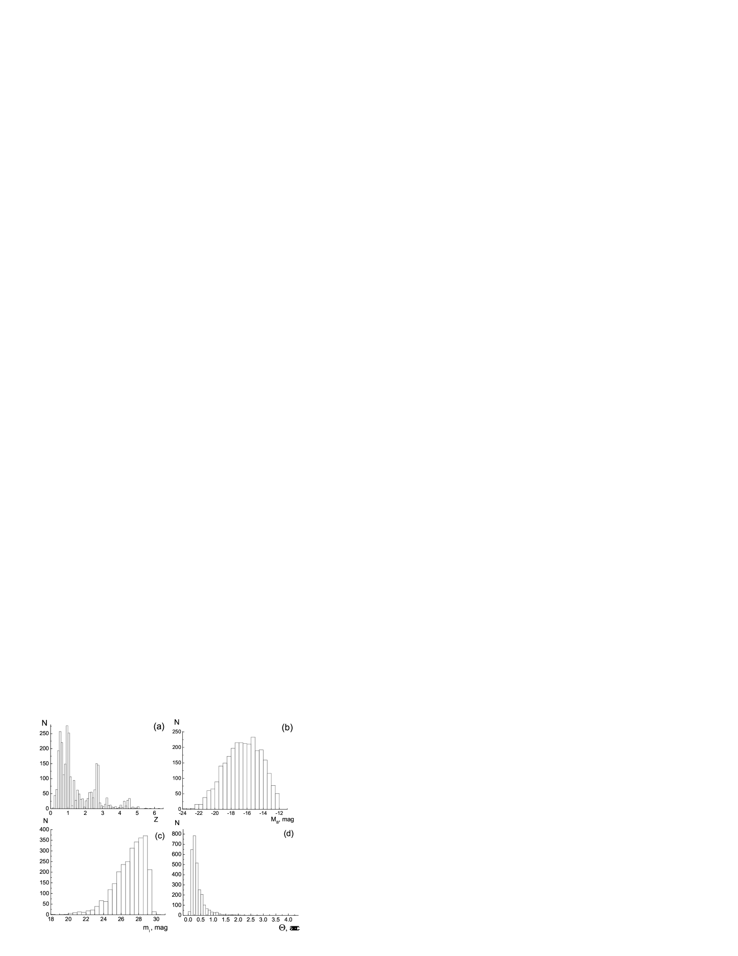
Figure 2: The distribution of the observed quantities of the galaxies of the catalog for the $C_{i}\_bviz\_mod3$ model, where (a) is the distribution of photometric redshifts; (b)—the distribution of B-band absolute magnitudes; (c)—the distribution of i-band apparent magnitudes, and (d)—the distribution of angular sizes.

The initial data (the zero approximation of the theoretical model of surface-brightness distribution) include:

• The coordinates of the center of the object;

• The total flux from the entire object in magnitudes;

• The $FWHM$ of the surface-brightness profile of the object;

• The axial ratio b/a of the galaxy;

• The position angle of the galaxy.

We computed the surface-brightness profile only for galaxies with absolute magnitudes $M$ ranging from -20 to -18 and with the 99-100% probability of photometric redshifts ($z_{phot}$) (it is one of the parameters in the general catalog of objects). After selecting objects from the catalog in accordance with the above criterion we studied the objects with $FWHM_{flux}>10$ pixels. We imposed this additional constraint on the sample in order to improve the convergence of the method that we use to find the surface-brightness profile.

As a result, we obtained a catalog of parameters for finding the surface-brightness profiles in the Gaussian approximation for each object of the sample considered.

III ANALYSIS OF THE GALAXY SAMPLE

III.1 Constructing the Main Catalog

We already mentioned above that after reducing the HUDF we constructed the general catalog of the objects. However, we then modified this catalog and drew various samples from it. To systematize the data, here we review the samples and catalogs.

Figure 3: The “absolute magnitude–linear size” relation for all galaxies of the sample $C_{i}\_bviz\_mod3$ with the parameters of standard cosmological model.

After the objects were identified by sExtractor, we constructed the preliminary catalog of data, $C_{i}\_bviz$. It contains the principal parameters (the coordinates, sizes, ellipticity, fluxes, etc.) for each object in the four filters B, V, z, i.

To find the photometric redshifts, we compiled the input catalog of data containing the magnitudes of the galaxies in the four filters and their color indices. We added the input data including $z_{ph}$ (photometric redshifts), $M$ (absolute magnitudes), and Galaxy Types into the the general data catalogs $C_{i}\_bviz\_mod1$, $C_{i}\_bviz\_mod2$, $C_{i}\_bviz\_mod3$, and $C_{i}\_bviz\_mod4$ corresponding to the cosmological models, $\Omega_{V}=0.0$ $\Omega_{m}=0.0$, $\Omega_{V}=0.0$ $\Omega_{m}=1.0$, $\Omega_{V}=0.7$ $\Omega_{m}=0.3$, and $\Omega_{V}=1.0$ $\Omega_{m}=0.0$. We then subscripted the name of the catalog depending on the absolute magnitude of objects selected from the main catalog: $M18\_20$ (galaxies with absolute magnitudes $M$ in the interval from –20 to –18) or $M20\_22$.

We the excluded from the resulting catalog of objects the galaxies with incorrectly computed flux in at least one of the filters (in these cases sExtractor outputs the the flux value equal to 99 magnitudes) and the probability of finding the photometric redshift $z_{ph}<90\%$.

III.2 Distribution of the Observed Parameters of the HUDF Galaxies

In Fig. 2 we represent the distribution of the observed parameters of the objects of the i-band catalog. The histograms of $\Theta$, $m$, $M$, and $z$ are computed for the galaxy sample of the $C_{i}\_bviz\_mod3$ catalog, which contains a total of 4125 objects.

It is evident from Fig. 2 that the distribution of photometric redshifts is significantly inhomogeneous (a); the distribution of absolute magnitudes $M$ lies in the interval from –24 to –12 (b); the number of galaxies increases with decreasing flux down to $29^{m}$, which corresponds to the completeness limit of the catalog (c); the characteristic angular size $\Theta$ is equal to $0.3^{\prime\prime}$ (d).

III.3 Constraints on Absolute Magnitudes

Figure 3 shows the “absolute magnitude—linear size” diagram for galaxies. We use the $FWHM_{flux}$ quantities, which correspond to the halfwidth of the flux profile, as the sizes of the corresponding galaxies.

The increase of linear size becomes slower for bright galaxies and therefore, to reduce the systematic displacement of the data points on the $\Theta(z)$ diagram, constraints are to be imposed on the absolute magnitudes of galaxies. The distribution of linear sizes of faint galaxies is uniform and therefore we exclude them in order to reduce the systematic errors. The vertical line in Fig.3 corresponds to the limiting absolute magnitude of galaxies included into the sample, which contains galaxies with absolute magnitudes brighter than –18. We compute the absolute magnitudes using formula (31), which already incorporates a fixed cosmological model and spectral energy distributions of galaxies. Therefore to estimate the evolution parameter k, we use the subsamples of galaxies limited by absolute magnitude in accordance with each particular cosmological model.

III.4 Division into Subsamples

We found the parameter of the evolution of linear sizes of galaxies as a function of their type and subdivided the sample into the subsamples of spiral and elliptical galaxies. HyperZ code determine the galaxy type by the form of its spectrum while computing the photometric redshifts. We selected the brightest galaxies of the catalog for various intervals of absolute magnitudes. We computed the absolute magnitude $M$ separately for each cosmological model. Then we subdivided the $C_{i}\_bviz$ catalog into four subsamples (in accordance to each cosmological model), which we then subdivided into subcatalogs: $-20\leq M\leq-18$; $-22\leq M\leq-20$.

IV THEORETICAL $\Theta(z)$ AND $J(z)$ RELATIONS

Many papers have been dedicated to the discussion of observational tests of cosmological models (see, e.g., the reviews by Sandage Sandage:Nabokov_n ; Sandage2:Nabokov_n ). Modern data are indicative of the need for the use of cosmological models including both dark matter and dark energy. In this section we give the general theoretical relations used to analyze the classical cosmological tests.

IV.1 The “Metric Distance–Redshift” Relation

The density parameter in the Friedmann cosmological models including cold dark matter (CDM) and dark energy is equal to the sum

$$\Omega=\Omega_{m}+\Omega_{V}\,,$$ (15)

where $\Omega_{m}=\rho_{m}/\rho_{crit}$ is the parameter of the density of cold matter and $\Omega_{V}=\rho_{V}/\rho_{crit}$ is the parameter of the density of dark energy, for which $p_{V}=w\rho_{V}c^{2}$, and $w\leq 0$. In the particular case $w=-1$ dark energy corresponds to cosmological vacuum and Einstein’s cosmological constant.

In the general case the Friedmann equation has the following form:

$$\Omega=1-\Omega_{k}\,,$$ (16)

or

$$H^{2}-\frac{8\pi G}{3}\rho=-\frac{kc^{2}}{S^{2}}\,,$$ (17)

where   $\Omega=\varrho/\varrho_{crit}$ is determined by the total density   $\varrho=\varrho_{m}+\varrho_{V}$; the critical density is $\varrho_{crit}=3H^{2}/8\pi G$, and the curvature density parameter is $\Omega_{k}=kc^{2}/S^{2}H^{2}$. The Hubble parameter $H=\dot{S}/S$ and the scale factor $S(t)$ are set by the Robertson–Walker four-interval, which has the following form:

$$ds^{2}=c^{2}dt^{2}-S^{2}(t)d\chi^{2}-S^{2}(t)I_{k}^{2}(\chi)(d\theta^{2}+\sin^{2}\theta d\phi^{2})\,,$$ (18)

where $I_{k}(\chi)=\sin(\chi),~{}\chi,~{}\sinh(\chi)$ with $k$ = +1, 0, and –1, respectively.

The proper metric distance $r$ from the observer to the galaxy with dimensionless comoving coordinate $\chi$ in metrics (18) is given by the following formula:

$$r(t,\chi)=S(t)\chi~{}.$$ (19)

Note that the proper metric distance $r\,\,$ (measured inside the three-dimensional hypersphere) and scale factor $S\,$ have the dimensions of length: $[r]=[S]=[cm]$ .

To describe the “angular size–redshift” relation, observational cosmology uses the “external”  metric distance $l$

$$l(t,\mu)=S(t)\mu~{},$$ (20)

where dimensionless comoving distance $\mu$ appears explicitly in the four-interval

$$ds^{2}=c^{2}dt^{2}-S^{2}(t)\frac{d\mu^{2}}{1-k\mu^{2}}-S(t)^{2}\mu^{2}(d\theta^{2}+\sin^{2}\theta d\phi^{2}).$$ (21)

According to formula (21), distance $l=S\mu$ is measured in the ambient four-dimensional space. The relation between $\chi$ and $\mu\,\,$ ($\chi=I_{k}^{-1}(\mu),~{}~{}\mu=I_{k}(\chi)$) can be used to write the relations between metric distances (19) and (20) in the following form

$$r=S(t)I^{-1}_{k}(l/S)\,,\qquad l=S(t)I_{k}(r/S)\,,$$ (22)

where $I^{-1}_{k}$ is the inverse function to $I_{k}$. At $k=0$ we have $r=l$.

The general formula for metric distance in the Friedmann model has the following form:

$$r(z)=\frac{c}{H_{0}}\int_{0}^{z}\frac{dz^{\prime}}{h(z^{\prime})}\,,$$ (23)

where $h(z)$ can be derived from the Friedmann equation in the following form:

$$h(z)=\sqrt{\tilde{\rho}(z)\Omega_{0}+(1-\Omega_{0})(1+z)^{2}}\,,$$ (24)

where $\Omega_{0}=\rho^{0}_{\rm tot}/\rho^{0}_{\rm crit}$ is the density parameter at the present epoch and $\tilde{\rho}(z)=\rho/\rho_{0}$ is the normalized total density of all components.

In case of the two-liquid dust + vacuum model (without interaction) the proper metric distance is given by the following formula:

$$r(z)=\frac{c}{H_{0}}\times\quad\quad\quad\quad\quad\quad\quad\quad\quad\quad\quad\quad\quad$$

$$\int_{0}^{z}\frac{dz^{\prime}}{\sqrt{(\Omega_{V}^{0}+\Omega_{m}^{0}(1+z^{\prime})^{3}-\Omega_{k}^{0}(1+z^{\prime})^{2})}}\,,$$ (25)

and the external metric distance is equal to (for $k=-1$):

$$l(z)=\frac{c}{H_{0}}\frac{1}{(-\Omega_{k}^{0})^{1/2}}\times\quad\quad\quad\quad\quad\quad\quad\quad\quad$$

$$\sinh\left(\int^{1}_{\frac{1}{1+z}}\frac{(-\Omega_{k}^{0})^{1/2}dy}{y\sqrt{(\Omega_{m}^{0}/y-\Omega_{k}^{0}+\Omega_{V}^{0}y^{2})}}\right).$$ (26)

In the $k=0$ case :

$$l(z)=\frac{c}{H_{0}}\int^{1}_{\frac{1}{1+z}}\frac{dy}{y\sqrt{(\Omega_{m}^{0}/y+\Omega_{V}^{0}y^{2})}}.$$ (27)

In the $k=+1$ case:

$$l(z)=\frac{c}{H_{0}}\frac{1}{(\Omega_{k}^{0})^{1/2}}\times\quad\quad\quad\quad\quad\quad\quad\quad\quad\quad$$

$$\sin\left(\int^{1}_{\frac{1}{1+z}}\frac{(\Omega_{k}^{0})^{1/2}dy}{y(\Omega_{m}^{0}/y-\Omega_{k}^{0}+\Omega_{V}^{0}y^{2})^{1/2}}\right).$$ (28)

IV.2 The “Angular Size–Redshift” Relation

The relation between metric distance $l(z)$ and angular size $\Theta$ has the following form:

$$\Theta(z)=d\left(\frac{1+z}{l(z)}\right)=\frac{d}{R_{H{}_{0}}}\left(\frac{1+z}{x(z)}\right),$$ (29)

where $d$ is the fixed size of the galaxy; $x(z)=l(z)/R_{H_{0}}$ and $R_{H{}_{0}}=c/H_{0}$, $H_{0}=72$   (km/s)/Mpc. If $\Theta$ is in arcsec and $d$ in kpc then formula (29) acquires the following form:

$$\Theta(z)=0.0481\times d\times\left(\frac{x(z)}{1+z}\right)^{-1}\,.$$ (30)

Figure 4: Comparison of theoretical models with observational data for galaxies in the interval of absolute magnitudes $M$ from –18 to –22 of the $C_{i}\_bviz\_el\_M18\_22$ sample. The dashed line corresponds to the theoretical model  $\Omega_{m}=1.0$ and $\Omega_{V}=0.0$; the solid line—to the model $\Omega_{m}=0.0\,\mbox{and}\,\Omega_{V}=0.0$; the dotted line—to $\Omega_{m}=0.3\,\mbox{and}\,\Omega_{V}=0.7$, and the dashed-and-dotted line—to $\Omega_{m}=0.0\,\mbox{and}\,\Omega_{V}=1.0$.

For different combinations of $\Omega_{m}$ and $\Omega_{V}$ metric distance $l(z)$ can be computed by formulae (IV.1 – IV.1).

IV.3 Absolute Magnitudes

To consider fixed intervals of galaxy luminosities, one must compute the absolute magnitudes of galaxies. In the Friedmann models the absolute magnitudes are computed using bolometric distance determined as $l_{bol}=l(z)\times(1+z)$. The absolute magnitude of the galaxy, $\>M_{j}$, in filter $j$ can be computed from the following general formula:

$$M_{j}=m_{j}-5\log\{l(z)(1+z)\}-25-\Delta M_{j}\,,$$ (31)

where distance $l(z)$ is in Mpc and $\Delta M_{j}=A_{j}+K_{j}+E_{j}$ is the correction to the absolute magnitude for extinction, redshift, and luminosity evolution.

IV.4 The “Surface Brightness–Redshift” Test

The “surface brightness–redshift” test is a critical one, because, as Tolman Tolman:Nabokov_n was the first to point out that the $J(z)$ relation is universal and the same for all Friedmann models.

It follows from the definition of the surface brightness of an object that:

$$J_{bol}=\frac{F_{bol}}{\Theta^{2}}=\frac{J_{0}}{(1+z)^{4}},$$ (32)

where $J_{bol}$ is the bolometric surface brightness; $F_{bol}$, the bolometric flux, and $J_{0}$, the surface brightness of the galaxy at z=0. In case of i-band we are dealing with the brightness observed in the given wavelength interval rather than with the bolometric brightness. Therefore below by $J_{bol}$ we mean $J_{obs}$ (observed in the the i filter). We then have:

$$\mu=\mu_{0}+2.5\log(1+z)^{4}+K_{i}(z)+E_{i}(z)=\mu_{0}+2.5\log(1+z)^{n},$$ (33)

where $\mu$ is the surface brightness measured in units mag${}^{{}^{\prime\prime}}$; $K_{i}(z)$, the K-correction to the i-band surface brightness; $E_{i}(z)$, the evolutionary correction to the i-band surface brightness; $n=4+p=$ $4+e_{k}+e_{e}$, and $p$, the combined parameter of the surface-brightness evolution.

V EVOLUTION OF SIZES AND SURFACE BRIGHTNESS

V.1 Parameter of the Evolution of Linear Sizes of Galaxies

Figure 4 compares the observational data for galaxies of the $C_{i}\_bviz\_el$ sample (here “el” indicates that the sample consists of elliptical galaxies) with theoretical models in the interval of absolute magnitudes $M$ from –22 to –18.

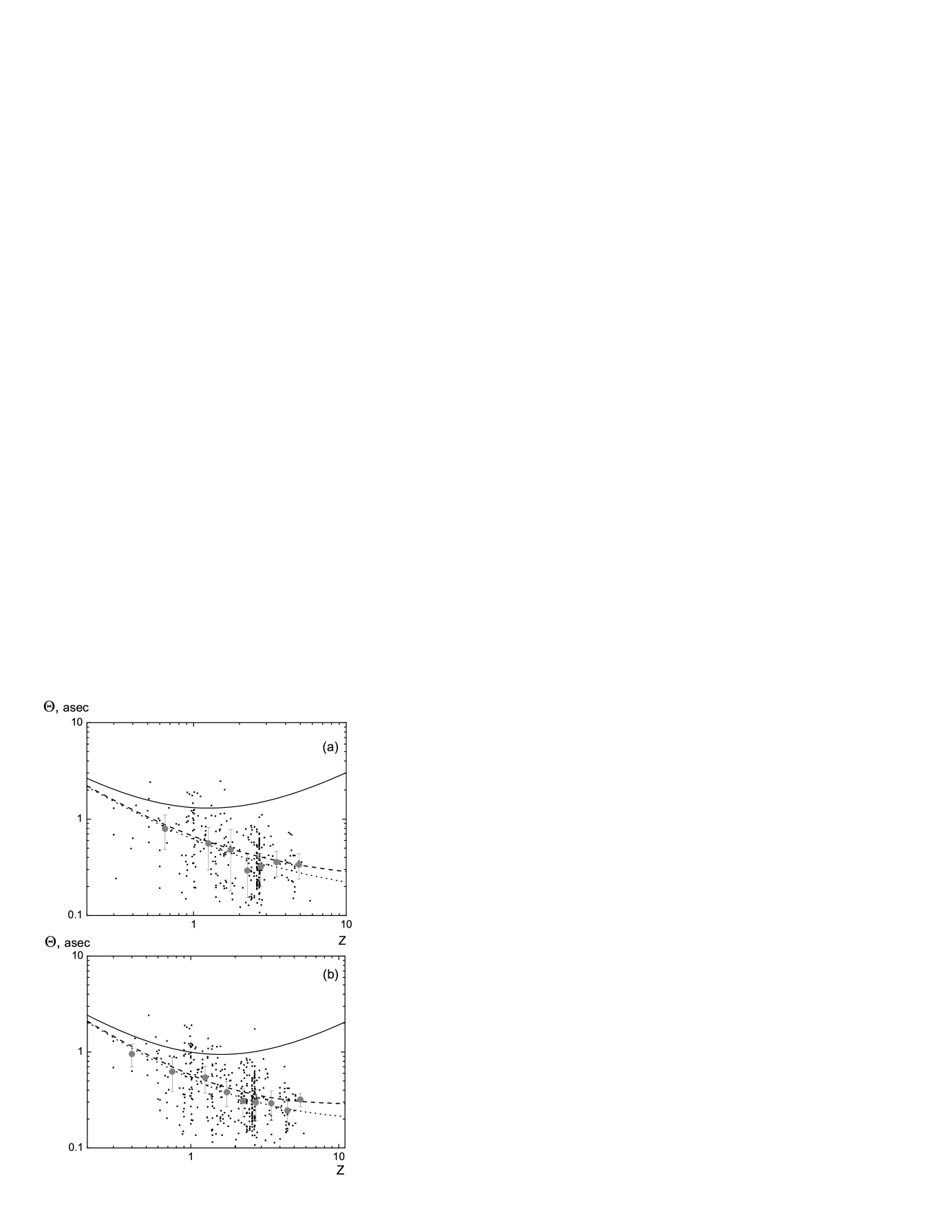
Figure 5: Finding the parameters of evolution for different models of galaxies with $M$ from –20 to –18 for the $C_{i}\_bviz\_mod3\_M18\_20$ (a) and $C_{i}\_bviz\_mod4\_M18\_20$ (b) samples. The solid line in plots (a) and (b) corresponds to the models with $\Omega_{m}=1.0,\,\Omega_{V}=0.0$ and $\Omega_{m}=0.3,\,\Omega_{V}=0.7$, respectively; the dashed line shows the fit for the entire sample, and the dotted line, the fit for median points.

It is evident from Fig. 4 that neither model passes through the median values for the given sample. This fact is usually explained by the evolution of linear sizes of galaxies and function $f(z)$ is introduced:

$$\Theta(z)_{obs}=f(z)\times\Theta(z)_{theor},$$ (34)

where $\Theta(z)_{obs}$ are the observed angular sizes and $\Theta(z)_{theor}$ are the theoretical angular sizes computed in terms of the model studied. The function usually has the form $f(z)=(1+z)^{k}$, where k is the parameter of evolution.

We compute the parameter of the evolution of galaxy sizes in accordance with formula (29). In Fig. 5 we present several plots for models with $\Omega_{m}$=1.0, $\Omega_{V}$=0.0 and $\Omega_{m}$=0.3,  $\Omega_{V}$=0.7. We determine parameter k by applying the method of least squares both to the values for the entire sample and to median points. We perform our computations using mathematical package Microcal Origin 7.0. Note that the median is a statistically more stable parameter than the mean. As a result, we find the parameter of the evolution of galaxy sizes for four models both for the sample with $M$ from –20 to –18 and for objects with $M$ from –22 to –20. Table 1 lists the results obtained for angular sizes.

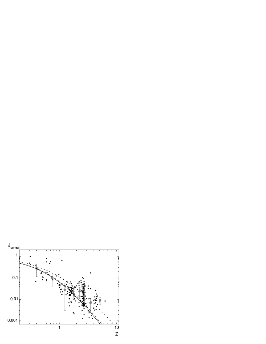
Figure 6: Evolution of surface brightness as a function of $z$ for the $C_{i}\_bviz\_mod3\_M20\_22$ sample. The dashed line corresponds to averaging over all points of the sample; the dotted line—to averaging over the median points; the solid line shows the theoretical evolution of surface brightness,and the vertical bars show the errors of the median values.

Note that we set parameter $d$ equal to 12 kpc for the sample of objects with $M$ from –22 to –20 (compared to $d$=8 kpc adopted for galaxies with $M$ from –20 to –18). This is due to the fact that bright galaxies (compared to galaxies with $M$ from –20 to –18) have slightly larger sizes. That is why we slightly increased the “fixed galaxy size”.

V.2 Surface Brightness Evolution

Figure 7: Surface brightness evolution as a function of $z$ for the $C_{i}\_bviz\_mod3\_M20\_22$ sample. The dashed line corresponds to averaging over all points of the sample, $p=-0.8251$; the dotted line corresponds to averaging over median points, $p=-0.1144$; the solid line shows the evolution of surface brightness, $p=0$, and the vertical bars show the errors of the median values.

The distribution of surface brightness values of the galaxies can be characterized by the $J(\Theta,z)$ profile for each $z$. In this paper we analyze the evolution of the surface brightness of galaxies, i.e., the central value of the $J(z)_{\Theta=0}$ profile found using sExtractor and GALFIT codes.

We determine the normalizing constant $J_{0}$ by averaging the surface-brightness values for galaxies with $z$ from 0 to 0.5. The surface-brightness parameter $n=4+p=4+$ k $+e_{J}$ is given by the following formula:

$$J_{norm}=\frac{1}{(1+z)^{n}},$$ (35)

where $J_{norm}$ is the normalized surface brightness: $J_{norm}$ = $J/J_{0}$ ($J_{0}$ is the central surface brightness of the given galaxy) and $p$ is the parameter of evolution. We determine parameter $n$ by applying the least-squares method both to all points and to the median values of normalized surface brightness. In Fig. 6 we compare the curves of the theoretical and observed evolution of surface brightness.

For better visualization, these curves can be drawn in other axes. We use formula (35) to change to surface brightness $\mu$ :

$$-2.5\lg(J_{obs}\Delta x^{-2})=-2.5\lg(J_{0}\Delta x^{-2})+2.5\lg(1+z)^{n},$$ (36)

whence it follows that

$$\mu_{obs}=\mu_{0}+2.5\,n\,\log(1+z),$$ (37)

where $\Delta x$ is the scale factor for converting pixels to acrseconds. In Fig. 7 we show the plots with different evolution parameters $p$ in the ($\mu~{}\mbox{vs.}~{}\lg(1+z)$) axes, and $\mu_{0}=17.89$ mag${}^{{}^{\prime\prime}}$.

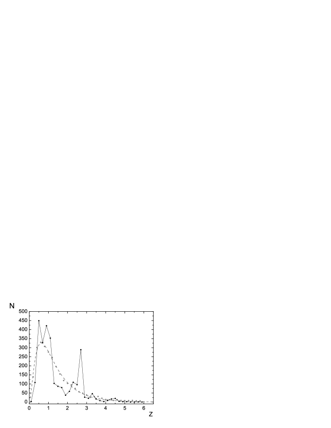
Figure 8: Observed (the solid line) and modeled (the dashed line) binned ($\Delta z=0.2$) redshift distributions.

The results of our analysis of the surface-brightness evolution of the galaxies of the HUDF field considered imply a surface-brightness evolution parameter of $p=-0.83\pm 0.1$ $(n=4+p=3.17\pm 0.1)$ if computed using all points of the sample and $p=-0.11\pm 0.1$ $(n=3.89\pm 0.1)$ if computed by using only median points for galaxies in the interval of absolute magnitudes $M$ from –18 to –20.

VI IDENTIFICATION OF POSSIBLE SUPERLARGE STRUCTURES IN THE RADIAL DISTRIBUTION OF HUDF GALAXIES

The distribution of photometric redshifts of HUDF galaxies in the z-interval from 0.1 to 6.5 can be searched for superlarge structures, which show up in the form of fluctuations of the number of galaxies within the corresponding bins of the distribution considered.

VI.1 Distribution of Photometric Galaxy Redshifts

As a model distribution of galaxies to compare with the observed distribution, we use a uniform distribution of points inside a unit-radius sphere. We randomly assigned to each point an absolute magnitude in accordance with the Schechter luminosity function:

$$\phi(L)dl=\phi^{*}{\left(\frac{L}{L^{*}}\right)}^{\alpha}\exp\left(-\frac{L}{L^{*}}\right)d\left(-\frac{L}{L^{*}}\right).$$ (38)

Our next step was to find the redshifts for modeled data points. To do this, we had to change from the radial distance unit to metric distance one. At $k=0$ (a zero-curvature space) the outer and inner metric distances coincide, $l(z)=r(z)$. We thus use the inverse relation $z=l^{-1}(z)$ and formula (27) to compute the redshift. To allow for selection due to the limit of telescope sensitivity, we limit the sample by apparent magnitude—it must not exceed $29^{m}$.

We fit the resulting model distribution by the following formula:

$$dN=Ax^{\alpha}\exp\left(-\frac{x}{x_{0}}\right)^{\beta}dz,$$ (39)

where the free parameters $\alpha$, $\beta$, and $x_{0}$ are inferred using the least squares method and $A$ is the normalizing constant.

Table 1: Results of computation of the parameter k of the evolution of angular sizes of the galaxies for different cosmological models

N	Model	Evolution parameter $k$		$M$(mag.)
		based on all points	based on median points
I.1	$\Omega_{m}=0.0,\Omega_{V}=1.0$	$-0.40\pm 0.03$	$-0.58\pm 0.09$	-20 -18
I.2	$\Omega_{m}=1.0,\Omega_{V}=0.0$	$-0.99\pm 0.04$	$-1.09\pm 0.05$	-20 -18
I.3	$\Omega_{m}=0.3,\Omega_{V}=0.7$	$-0.79\pm 0.03$	$-0.91\pm 0.05$	-20 -18
I.4	$\Omega_{m}=0.0,\Omega_{V}=0.0$	$-0.67\pm 0.03$	$-0.89\pm 0.18$	-20 -18
II.1	$\Omega_{m}=0.0,\Omega_{V}=1.0$	$-0.49\pm 0.06$	$-0.60\pm 0.08$	-22 -20
II.2	$\Omega_{m}=1.0,\Omega_{V}=0.0$	$-1.14\pm 0.10$	$-1.32\pm 0.12$	-22 -20
II.3	$\Omega_{m}=0.3,\Omega_{V}=0.7$	$-0.90\pm 0.08$	$-1.07\pm 0.06$	-22 -20
II.4	$\Omega_{m}=0.0,\Omega_{V}=0.0$	$-0.75\pm 0.08$	$-0.85\pm 0.12$	-22 -20

VI.2 Comparison of the Expected and Observed Distributions

In Fig. 8 we present the observed and modeled (according to (39)) redshift distributions of HUDF galaxies. The parameters of the modeled distribution are $\alpha=2.84$, $\beta=0.48$, $x_{0}=0.015$.

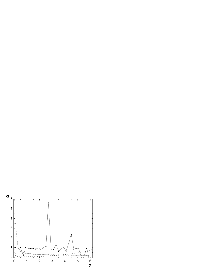
Figure 9: Observed (the solid line), theoretical (the dashed line), and Poisson (the dotted line) deviations of photometric redshifts in $\Delta z=0.2$ bins.

We use the following quantity to measure the deviation of the observed number of galaxies from the theoretically expected numbers:

$$\sigma_{obs}=\frac{|N_{obs}-N_{theor}|}{N_{theor}},$$ (40)

where $N_{theor}$ is the expected (according to (39)) number of galaxies in the interval of redshifts from $z$ to $z+\Delta z$ and $N_{obs}$ is the number of galaxies observed in the same interval.

The theoretically expected amplitude of fluctuations is characterized by the dispersion of Poisson noise, $\sigma_{{}_{P}}=1/N_{theor}$, and the dispersion associated with correlated structures, which we computed by the following formula Peebles:Nabokov_n :

$$\sigma_{theor}^{2}=\frac{J_{2}}{1+z}\,\left(\frac{r_{0}}{r_{eff}}\right)^{\gamma},$$ (41)

where $\gamma=1.8$; $J_{2}=72.0/[2^{\gamma}(3-\gamma)(4-\gamma)(6-\gamma)]$=1.865; $r_{0}=5$ Mpc; $r_{eff}=(3/4\pi r^{2}\Delta rS)^{\frac{1}{3}}$ is the effective radius corresponding to the volume of the interval; $\Delta r$ corresponds to the $dz$ layer, and S is the solid angle of the HUDF field.

In Fig. 9 we present the plot of observed deviations $\sigma_{obs}$ and theoretically expected deviations $\sigma_{p},\sigma_{theor}$ from uniform distribution of galaxies.

VII DISCUSSION OF THE RESULTS AND THE MAIN CONCLUSIONS

Our analysis of the classical cosmological test $\Theta(z)$ shows that the choice of cosmological models has a strong effect on the parameter of the evolution of linear sizes of galaxies.

It is evident from Table 1 that the parameter of the evolution of linear sizes for galaxies with absolute magnitudes in interval from –20 to –18 varies from k$=-0.40\pm 0.03$ for the model with $\Omega_{m}=0.0$  and  $\Omega_{V}=1.0$ to k$=-1.09\pm 0.06$ for the model with $\Omega_{m}=1.0$ and $\Omega_{V}=0.0$. This parameter varies from $-0.49\pm 0.06$ to $-1.32\pm 0.12$ for galaxies with luminosities in the interval from –22 to –20. The inferred values of parameter k agree with the results of Bowens et al. Bouwens:Nabokov_n for other samples of galaxies from HDF-S, HDF-N, GOODS, and HUDF. The above authors used a cosmological model with parameters $\Omega_{m}=0.3\,,\,\Omega_{V}=0.7$. For galaxies with luminosities in the interval of absolute magnitudes $M$ from -22.38 to -21.07 the parameter of galaxy size evolution was found to be k$=-1.05\pm 0.21$. For our sample parameter k$=-1.07\pm 0.06$ in case of $\Omega_{m}=0.3,\,\Omega_{V}=0.7$. Note that the $\Theta(z)$ diagram may become an efficient cosmological test when a reliable model of the evolution of galaxy sizes is developed.

The surface brightness evolution parameter $p=-0.11\pm 0.1~{}(n=3.89\pm 0.1)$ inferred from the median points for galaxies in the absolute magnitude ($M$) interval from -18 to -20 requires further analysis. This is due to the fact that the K-correction to the surface brightness includes a combination of the K-correction to the flux and the K-correction to the angular size.

An analysis of the distribution of HUDF galaxies reveals strong deviations of the observed number of galaxies from the number of galaxies expected for a uniform distribution. The observed irregularities correspond to a scale length of about 2000 Mpc. This may be due both to real superlarge structures and to hidden selection effects that show up in finding the photometric redshifts. This problem requires further analysis.

- (1) E. Hubble and R. Tolman, Astrophys. J. 82, 302 (1935).
- (2) A. Sandage, Astrophys. J. 133, 355 (1961).
- (3) A. Sandage, In The Deep Universe (Berlin, Springer-Verlag, 1995).
- (4) D. N. Spergel, R. Bean, O. Dore, and M. R. Nolta, APJS 170, 377 (2007).
- (5) A. Clocchiatti, P. Schmidt, and A. Filippenko, Astrophys. J. 642, 1 (2006).
- (6) A. Conley, G. Goldhaber, L. Wang, and G. Aldering, Astrophys. J. 644, 1 (2006).
- (7) E. Bertin and S. Arnouts, AAS 117, 393 (1996).
- (8) M. Bolzonella, J.-M. Miralles, and R. Pello’, AAA 363, 476 (2000).
- (9) G. D. Coleman, C. C. Wu, and D. W. Weedman, APJS 43, 393 (1980)
- (10) D. Calzetti, L. Armus, R. C. Bohlin, and A. L. Kinney, Astrophys. J. 533, 682 (2000).
- (11) J. B. Oke and D. G. Korycansky, Astrophys. J. 255, 11 (1982).
- (12) Y. Peng Chien, Steward Observatory, University of Arizona, User’s manual, GALFIT v2.0.
- (13) Yu. V. Baryshev, F. Sylos Labini, M. Montuori, and L. Pietronero, Vistas in Astronomy 38, 419 (1994).
- (14) R. J. Bouwens, G. D. Illingwort, L. P. Blakeslee, and T. J. Broadhurst, Astrophys. J. 611, L1 (2004).
- (15) J. E. Peebles, The large-scale structures of the Universe (Princeton University Press, 1980).