Evolve Networks Towards Better Performance: a Compromise between Mutation and Selection

Abstract

The interaction between natural selection and random mutation is frequently debated in recent years. Does similar dilemma also exist in the evolution of real networks such as biological networks? In this paper, we try to discuss this issue by a simple model system, in which the topological structure of networks is repeatedly modified and selected in order to make them have better performance in dynamical processes. Interestingly, when the networks with optimal performance deviate from the steady state networks under pure mutations, we find the evolution behaves as a balance between mutation and selection. Furthermore, when the timescales of mutations and dynamical processes are comparable with each other, the steady state of evolution is mainly determined by mutation. On the opposite side, when the timescale of mutations is much longer than that of dynamical processes, selection dominates the evolution and the steady-state networks turn to have much improved performance and highly heterogeneous structures. Despite the simplicity of our model system, this finding could give useful indication to detect the underlying mechanisms that rein the evolution of real systems.

I Introduction

The successful application of evolutionary process Barabási and Albert (1999); Watts and Strogatz (1998) to the explanation of real networks, was one of the major achievements in the research of complex networks. Meanwhile, the topological structure of complex networks was frequently found to have determinative effect on the dynamical processes running on themDerrida and Pomeau (1986); Pastor-Satorras and Vespignani (2001); Boccaletti et al. (2002), and vice versaBi and Poo (2001). Therefore, many dynamical systems were modeled as adaptive networks, in which feedback from dynamical processes was extensively coupled into the structural evolutionsHolme and Newman (2006); Garlaschelli et al. (2007); Gross and Blasius (2008). In most of these networks, the compositional elements could actively change their interaction subjects according to the dynamical states. But for many biological networks, structural mutation happened blindly and randomly, with a timescale much separated from that of dynamical processesJacob (1977); Sole et al. (2003). Besides, the structural evolution of these systems was mainly driven by preferential selection, in which systems exhibiting better performance during the life circle could pass their structural information to future generations with higher probabilityDarwin (1859). Thus, an important issue emerged: how intensively could the pursuit of specific performance, such as reaching functional states rapidly and robustlySiegal and Bergman (2002), reshape the topological structures via preferential selection?

In this paper, we investigate this question by designing a simple model system, in which we evaluate a network by its efficiency of escaping from disordered states in Local-Majority-Rule (LMR) dynamical processesZhou and Lipowsky (2005) and try to evolve networks of low efficiency towards networks of high efficiency via repeated mutations and selectionsStern (2003); Oikonomou and Cluzel (2006). Although LMR dynamics is too simple to represent most of the dynamical processes running on real systems, it could make the evolution only focus on optimizing the distribution pattern of edges among vertices, which greatly reduces the complexity of our problem. In the model system, we find the steady state of evolution depends strongly on the timescales of mutations and dynamical processes. When their timescales are comparable to each other, mutation dominates the evolution and the steady-state networks have similar structure as the steady-state networks of pure mutations. On the opposite hand, when the timescale of mutations is much longer than that of dynamical processes, selection dominate the evolution and highly heterogeneous networks with heavily connected hub and much improved efficiency emerge from the evolution. In the extreme situation, networks with optimal efficiency, which also deviate significantly from the steady-state networks of pure mutations in topological structure. At the end of this paper, we also propose a simple model on the evolution of particles. Additionally, we illustrate that this conclusion is still valid even in infinite population limit by a simple mathematical model. As an extension, this finding calls for a comprehensive understanding of the evolution of real systems, which is consistent with the suggestion that the effect of likelihood should be also incorporatedWhitfield (2007).

II Results

In the evolution with low mutation rate ($\mu=0.01$), the networks evolve to have highly heterogeneous structures (Fig. 1.[a]), in which a vertex with degree comparable to network size $N$ emerges to act as the communicating hub. Meanwhile, the degree distribution of the other vertices shifts to be power-law-like for small degrees, which is significantly different from the exponential degree distribution of the steady-state networks under pure mutation. Besides, these highly heterogeneous networks exhibit strong degree-degree correlations indicated by two parameters $R\approx-0.495\pm 0.025$, which means the global hub prefers intensively to interact with vertices having low degrees, and $r\approx 0.067\pm 0.0083$, which means the other vertices prefer to connect with vertices having similar degrees. We notice that such degree-degree correlations are consistent with the spin-spin correlations embedded in the strongly disordered spin configurations of highly heterogeneous networks. In other words, the dynamics-driven evolution is able to detect the correlation between different vertices’ states and transfer it to topological clustering, which gives another potential explanation to the community-rich structures of many biological and social networks.

Figure 1: The steady-state network under dynamics-driven evolution with different mutation rate $\mu=0.01$ (a) or $\mu=1$ (b) shows different vertex-degree distributions. Both of the networks are of size $N=2000$, average connectivity $\langle k\rangle=10$ and minimal vertex-degree $k_{0}=3$. The solid lines represent the corresponding degree distribution for steady-steady networks under pure mutation (averaged over $200$ samples), while the dashed line in (a) is the best power-law fit $P(k)\sim k^{-1.92\pm 0.02}$ for the degree distribution of non-global hub vertices.

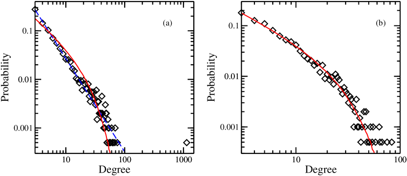
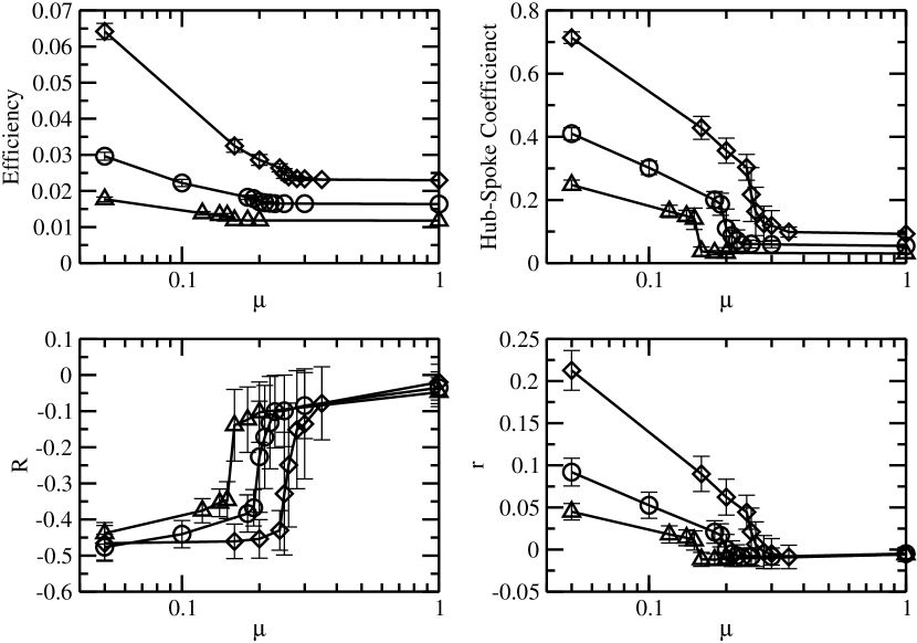
On the opposite side, in the dynamics-driven evolution with high mutation rate ($\mu=1$) selection fails to achieve further improvement in both efficiency and structure than mutation-driven evolution, and the networks remain similar to the steady-state networks under pure mutations (Fig. 1.[b]). From extensive simulations, we find there exists a critical mutation rate $\mu_{c}$ which classifies the dynamics-driven evolutions with different mutation rate into two distinct regimes (Fig. 2). In the regime $\mu>\mu_{c}$, mutations dominate the evolution, and the steady-state networks have similar structure as the steady-state networks under pure mutation. While in the regime $\mu<\mu_{c}$, the steady-state networks appear to have highly heterogeneous structures, and their improvement in both efficiency and structure grows monotonically as $\mu$ decreased. Importantly, the critical mutation rate $\mu_{c}$ decreases rapidly with $N$, which indicates a growing difficulty for large networks to achieve apparent optimization via dynamics-driven evolution.

Figure 2: Transition of the steady-state mean efficiency $\mathcal{E}$, mean hub-spoke coefficient $C_{hs}$, mean correlation index $R$ and mean assortative-mixing index (of global hub-removed subnetwork) $r$ under dynamics-driven evolution versus mutation rate $\mu$. The critical mutation rate $\mu_{c}=0.25$, $0.2$, $0.15$ for network size $N=500$ (diamonds), $1000$ (circles), $2000$ (squares), respectively. Each point represents a average over $6\times 10^{4}$ generations after the steady state of evolution is reached.

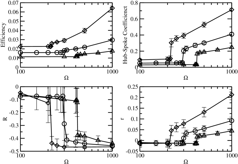
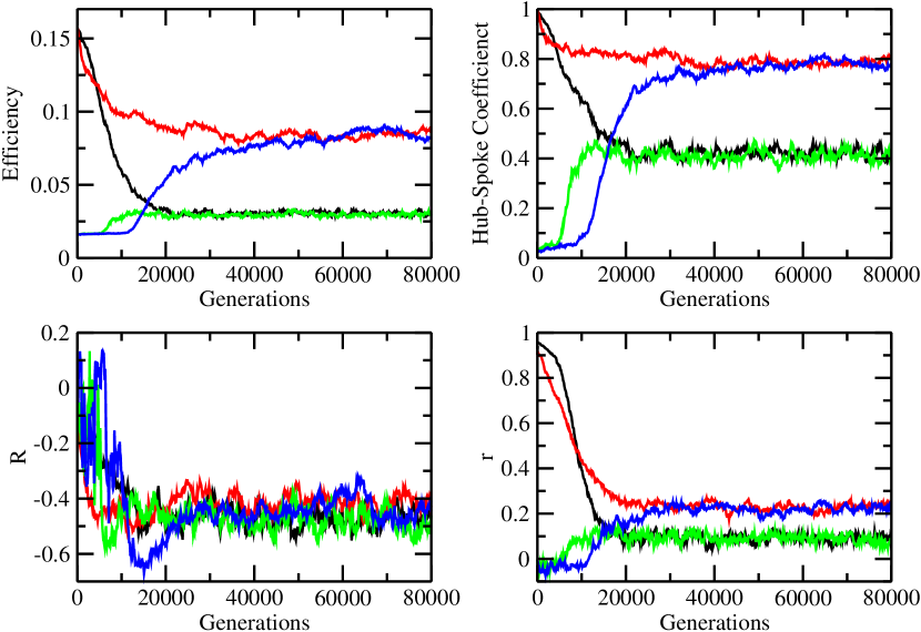
Interestingly, for the dynamics-driven evolutions with different sampling number $\Omega$, which determines the accuracy of efficiency sampling, similar transition emerges again (Fig. 3): only in the regime $\Omega>\Omega_{c}$, highly heterogeneous networks emerge and their improvement grows monotonically with $\Omega$; besides, the critical sampling number $\Omega_{c}$ increases rapidly with $N$. Thus, we conclude that the dynamics-driven evolution is determined by the balance of two counteracting effects: the promotive effect generated from preferential selection struggles to push the population towards networks with high efficiency, while the degradative effect brought together by random mutation and imprecise sampling of efficiency drives the population back to the steady-state networks under pure mutations. Consequently, the steady state of dynamics-driven evolution should be independent of the original networks, even when they are optimally designed (Fig. 4).

Figure 3: Transition of the steady-state mean efficiency $\mathcal{E}$, mean hub-spoke coefficient $C_{hs}$, mean correlation index $R$ and mean assortative-mixing index (of global hub-removed subnetwork) $r$ under dynamics-driven evolution versus sampling number $\Omega$. The critical sampling number $\Omega_{c}=220$, $300$, $420$ for network size $N=500$ (diamonds), $1000$ (circles), $2000$ (squares), respectively. Each point represents a average over $6\times 10^{4}$ generations after the steady state of evolution is reached.

Figure 4: (Color Online) The evolution of mean efficiency $\mathcal{E}$, mean hub-spoke coefficient $C_{hs}$, mean correlation index $R$ and mean assortative-mixing index (of global hub-removed subnetwork) $r$ as a function of simulation generations. The mutation rate is $\mu=0.05$ (black and green curves) or $\mu=0.01$ (red and blue curves). In the dynamics-driven evolution started from hub-spoke networks (black and red curves), the population is refreshed mostly by degraded networks due to their dominant fraction in the offsprings, and gradually converged the steady state of dynamics-driven evolution started from random Poissonian networks (green and blue curves).

To give a mathematical illustration, we consider a population of $M$ particles with two possible energy states $\varepsilon_{1}=0$ and $\varepsilon_{2}=1$. For a particle with energy $\varepsilon_{i}$ ($i=1$ or $2$), it will be assigned with an random evaluation following normal distribution

$$\mathcal{N}(\varepsilon_{i},\frac{\sigma^{2}_{i}}{\Omega})=\frac{1}{\sigma_{i}}\sqrt{\frac{\Omega}{2\pi}}e^{-\Omega(x-\varepsilon_{i})^{2}/(2\sigma_{i}^{2})},$$ (1)

here the standard deviation coefficient $\sigma_{i}$ satisfies $1\ll\sigma_{i}^{2}\ll+\infty$ and $\Omega\in[1,+\infty)$ is the control parameter. Besides, the offspring particle generated from a particle with energy $\varepsilon_{i}$ will appear on the opposite energy level with probability $p_{i}$, otherwise it will have identical energy with its parent. For mutation-driven evolution, every particle is replaced by an offspring generated from it at each generation. Easily seen, the particle composition $r_{g}$, which is defined to be the fraction of particles with energy $\varepsilon_{2}$ at generation $g$, will finally evolve to a steady state

$$r_{s}^{m}=\frac{p_{1}}{p_{1}+p_{2}}.$$ (2)

While in evaluation-driven evolution, every particle generates $E$ offsprings ($E$ is positive and finite) at the start of each generation, then only the $M$ particles with the highest evaluation of all $(E+1)M$ particles will survive and pass into next generation. Therefore, in the infinite population limit ($M\rightarrow\infty$), the steady-state particle composition $r_{s}^{e}$ will satisfy

$$\left\{\begin{array}[]{ll}r_{s}^{e}=[r_{s}^{e}+E(1-r_{s}^{e})p_{1}+Er_{s}^{e}(1-p_{2})]\int_{\phi_{s}}^{+\infty}\mathcal{N}(\varepsilon_{2},\frac{\sigma_{2}^{2}}{\Omega})dx\\ 1-r_{s}^{e}=[1-r_{s}^{e}+E(1-r_{s}^{e})(1-p_{1})+Er_{s}^{e}p_{2}]\int_{\phi_{s}}^{+\infty}\mathcal{N}(\varepsilon_{1},\frac{\sigma_{1}^{2}}{\Omega})dx\end{array}\right.,$$ (3)

here $\phi_{s}$ is the steady-state threshold that only particles with evaluation higher than it could survive. When $\Omega\rightarrow+\infty$, which means the stochastic fluctuation in particle evaluation will decrease to vanish, we find that $\int_{\phi_{s}}^{+\infty}\mathcal{N}(\varepsilon_{1},\frac{\sigma_{1}^{2}}{\Omega})dx\rightarrow\int_{\varepsilon_{2}}^{+\infty}\mathcal{N}(\varepsilon_{1},0)dx=0$ and $r_{s}^{e}\rightarrow 1$. Oppositely, when $\Omega$ is sufficient small so that

$$\int_{\phi_{s}}^{+\infty}\mathcal{N}(\varepsilon_{1},\frac{\sigma_{1}^{2}}{\Omega})dx\approx\int_{\phi_{s}}^{+\infty}\mathcal{N}(\varepsilon_{2},\frac{\sigma_{2}^{2}}{\Omega})dx,$$ (4)

which implies particles with different energy will survive with approximately equal probability, the steady-state composition will have $r_{s}^{e}\approx\frac{p_{1}}{p_{1}+p_{2}}=r_{s}^{m}$. On the other hand, in the extreme condition $p_{1}\rightarrow 0$ and $p_{2}\rightarrow 1$, which corresponds to the dynamics-driven evolution with high mutation rate, it could be derived from equation (2) and equation (3) that $r_{s}^{e}\rightarrow 0$ and $r_{s}^{m}\rightarrow 0$. In other words, the steady-state population of evaluation-driven evolutions has similar composition with that of mutation-driven evolution. However, in the extreme condition $p_{1}\approx p_{2}\ll 1$, which corresponds to the dynamics-driven evolution with small mutation rate, we find that $r_{s}^{e}\approx 1$ and $r_{s}^{m}\approx\frac{1}{2}$. Obviously, this compositional difference indicates an apparent optimization achieved by evaluation-driven evolution. Thus, if we take the dynamics-driven evolution as particles jumping among a series of structural heterogeneity levels, it could be easily derived from above analysis that the optimal structure could be approached only when the timescale of mutations is much longer than that of dynamical processesShao and Zhou (2008).

Finally we replace the local rewiring scheme by preferential rewiring, and show there also exists a critical strength $\beta_{c}$ (Fig. 5) to classify dynamics-driven evolutions with different strength of preferential rewiring into mutation-dominating regime ($\beta<\beta_{c}$) or selection-dominating regime ($\beta>\beta_{c}$). Interestingly, the critical strength $\beta_{c}$ is found to increase monotonically with $N$ as well, which reemphasizes the growing difficulty to achieve apparent optimization in large networks and supports that our finding is independent of the way how mutation occurs.

Figure 5: Transition of the steady-state mean efficiency $\mathcal{E}$, mean hub-spoke coefficient $C_{hs}$, mean correlation index $R$ and mean assortative-mixing index (of global hub-removed subnetwork) $r$ under dynamics-driven evolution versus the strength of preferential rewiring $\beta$. The critical strength $\beta_{c}=0.9$, $0.95$, $0.99$ for network size $N=500$ (diamonds), $1000$ (circles), $2000$ (squares), respectively. Each point represents a average over $6\times 10^{4}$ generations after the steady state of evolution is reached.

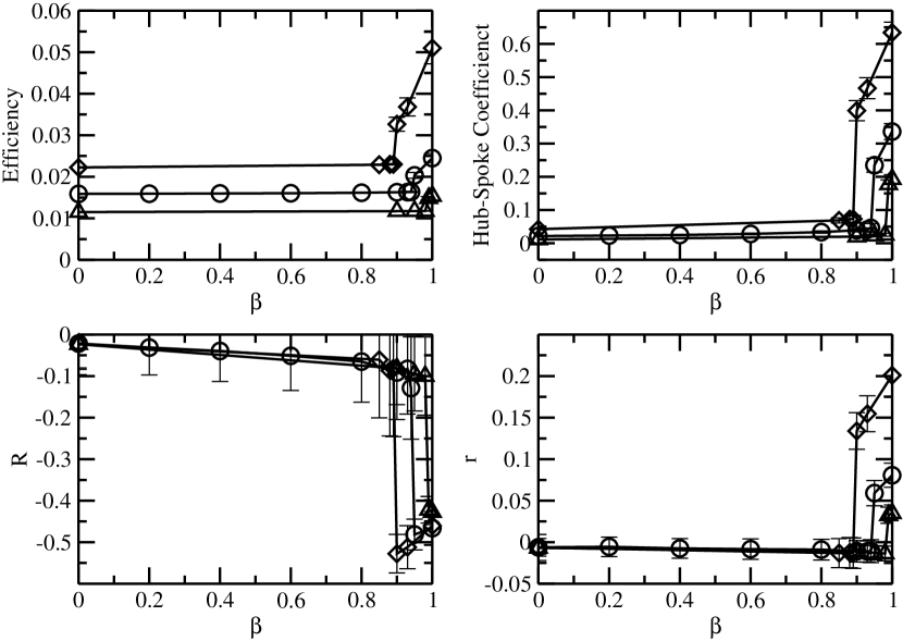
III Discussion

It has been debated whether the evolution in biological world should be viewed as some hill-climbing processWright (1982), or is mainly determined by the ”neutral mutations”Kimura (1983) like a random walk. But in our simple model system, we find when the optimal networks deviate from the steady state networks under mutations, a flexible combination of these two viewpoints is required. Interestingly, similar deviations are frequently detected in biological and social systems, such as the abundance of certain network motifsMilo et al. (2002) or nucleotide typesHallin and Ussery (2004). Therefore, dynamics-driven evolution could be a potential way to explain these structural heterogeneities. However, the evolution of real systems is far more complicated than our simple model system. Meanwhile, the evaluation of them is usually determined by a combination of multiple components such as efficiency, sensitivity, robustness and costMathias and Gopal (2001). Therefore, more detailed models are still needed to give a comprehensive understanding to the evolution running in real world.

IV Methods

IV.1 Local-Majority-Rule dynamics

For a undirected network of size $N$ and average connectivity $c$, we attach to each vertex $i$ a binary spin variable $\sigma_{i}=\pm 1$. At each time step $t$ of the LMR dynamics, all the vertices update their states synchronously according to

$$\sigma_{i}(t)={\rm sign}[\sum\limits_{j\in\partial i}\sigma_{j}(t-1)],$$ (5)

here $\partial i$ means the vertices which are connected with vertex $i$ directly. As described in Shao and Zhou (2008), we start a LMR dynamical process from a strongly disordered configuration ${\vec{\sigma}}(0)\equiv\{\sigma_{1}(0),\sigma_{2}(0),\ldots,\sigma_{N}(0)\}$, which is randomly generated with the constraints $\sum\limits_{i=1}^{N}\sigma_{i}=\sum\limits_{i=1}^{N}k_{i}\sigma_{i}=0$ ($k_{i}$ is the degree of vertex $i$). Typically, the LMR dynamics will drive the network to stabilize at a consensus state, in which all the vertices have the same spin state. It has been shown in Zhou and Lipowsky (2005) that in LMR dynamical processes, scale-free networks with degree distribution $P(k)\sim k^{-\gamma}$ and $\gamma\rightarrow 2$ can reach consensus more rapidly than Poissonian networks of similar size and average connectivity. In other words, highly heterogeneous networks are more efficient in communicating internal states than homogenous networks.

IV.2 Definition of efficiency

For a given network ${\cal G}$, we start a total number of $\Omega$ different LMR dynamical processes, and run them for $T=1$ time step to reach the corresponding configuration $\vec{\sigma}^{\alpha}(1)$. It has been shown in Zhou and Lipowsky (2005) that the characteristic relaxation time of a network in the LMR dynamics is determined by the the escaping velocity of the network’s spin configuration from the strongly disordered region. In this paper, we define the efficiency ${\cal G}$ of network ${\cal G}$ as the average change of vertex-state in $\vec{\sigma}(1)$, which is calculated according to

$$\mathcal{E}({\cal G})=\frac{1}{\Omega}\sum\limits_{\alpha=1}^{\Omega}\Biggl{|}\frac{1}{N}\sum\limits_{i=1}^{N}\sigma^{\alpha}_{i}(1)\Biggr{|}\ .$$ (6)

Easily seen, the efficiency sampled in this way is only a random estimation of the true efficiency $\mathcal{E}^{*}({\cal G})=\lim\limits_{\Omega\rightarrow\infty}\mathcal{E}({\cal G})$. According to the Central Limit Theorem, the distribution of $\mathcal{E}({\cal G})$ will be approximately Gaussian-distribution-like with the average value equal to $\mathcal{E}^{*}({\cal G})$, while the mean square variance will be proportional to $1/\Omega$ (see the Supplementary Information). That’s to say, the efficiency of a network will be evaluated more precisely with large $\Omega$.

IV.3 Evolutionary algorithm

The dynamics-driven evolution starts from a population of $P$ networks, which are uniformly sampled from the ensemble of random Poissonian networks of given size $N$ and average connectivity $\langle k\rangle$. At the beginning of each generation, every network generates $E$ exact copies, which expands the population to a size (E + 1)P. Then every new network undergoes random mutations following local rewiringBaiesi and Manna (2003):

1. For each vertex, mutation occurs with probability $\mu$ (mutation rate);

2. if mutation is accepted by vertex $i$, a rewiring of edge $(i,j)\rightarrow(i,l)$ is proposed, in which vertex $j$ is randomly selected from the nearest neighbors of vertex $i$ and vertex $l$ is then randomly selected from the nearest neighbors of vertex $j$ except vertex $i$;

3. this proposal will be rejected if and only if edge $(i,l)$ already exists or the degree of vertex $j$ is less than a minimal value $k_{0}$ after cutting edge $(i,j)$.

Then the efficiency of each network is sampled independently, and the population shrink to its original size with only $P$ networks with the highest efficiency survive and pass into next generation. As a reference to the dynamics-driven evolution, we also derive the steady-state networks under pure mutations by proposing a mutation-driven evolution. In the evolution, all the networks keep to be replaced by a new network generated from it following the same rules of mutation. For the local rewiring scheme, the degree distribution of the steady-state networks under pure mutations is shown to decay exponentiallyBaiesi and Manna (2003). If not specified by the context, the parameters default to adopt value $\Omega=1000$, $P=25$, $N=1000$, $\langle k\rangle=10$ , $E=3$ and $k_{0}=5$.

In this work we also involved preferential rewiring schemeOhkubo and Yasuda (2005): the only change from above description is that vertex $l$ ($l\neq i$ and $l\neq j$) in the rewiring proposal is chosen randomly with a probability $\Pi_{l}\propto(k_{l}+1)^{\beta}$, here $k_{l}$ is vertex $l$’s degree and $\beta$ is the control parameter which determines the strength of preferential rewiring. Obviously when $\beta=0$, the preferential rewiring scheme will degrade to random rewiring, under which the steady-state networks has been proved to be PoissonianOhkubo and Yasuda (2005). On the opposite side, the maximal value of $\beta$ used in this paper is $1$, under which the steady-state networks will have exponential degree distributionsOhkubo and Yasuda (2005).

IV.4 Identification of global hub and Definition of hub-spoke coefficient

For generality, we identify the vertex with the highest degree in a network as the global hub for both heterogeneous and homogenous networks. (If there are multiple vertices with the highest degree, we only identify the one with the smallest index as the only global hub.) We also define the hub-spoke coefficient $C_{hs}$ of a network to be $C_{hs}=\frac{k_{hub}}{N-1}$, in which $k_{hub}$ is the global hub’s degree and $N$ is network size. Obviously, when $C_{hs}$ equals to $1$, the network will look completely hub-and-spoke like.

IV.5 Quantification of degree-degree correlation in networks

To give an explicit quantification of the degree-degree correlations in a network, we define two quantities: correlation index $R$ measures the degree-degree correlation on links connecting the global hub and the other vertices, while assortative-mixing index $r$ measures the degree-degree correlations on links connecting the other vertices. We define $R$ to be the normalized ratio of the mean degree of nearest neighbors of the global hub $\langle k_{nn}^{hub}\rangle$ to the averaged value $\langle k_{nn}^{hub}\rangle_{ran}$ of this mean degree over an ensemble of randomly shuffled networksMilo et al. (2002), and calculate it according to

$$R=\left\{\begin{array}[]{ll}(\langle k_{nn}^{hub}\rangle-\langle k_{nn}^{hub}\rangle_{ran})/(\langle k_{nn}^{hub}\rangle_{max}-\langle k_{nn}^{hub}\rangle_{ran}),\;\mathrm{if}\;\langle k_{nn}^{hub}\rangle>\langle k_{nn}^{hub}\rangle_{ran}\\ (\langle k_{nn}^{hub}\rangle-\langle k_{nn}^{hub}\rangle_{ran})/(\langle k_{nn}^{hub}\rangle_{min}-\langle k_{nn}^{hub}\rangle_{ran}),\;\mathrm{if}\;\langle k_{nn}^{hub}\rangle<\langle k_{nn}^{hub}\rangle_{ran}\\ 0,\;\mathrm{if}\;\langle k_{nn}^{hub}\rangle=\langle k_{nn}^{hub}\rangle_{ran}\end{array}\right.,$$ (7)

here $\langle k_{nn}^{hub}\rangle_{max}$ and $\langle k_{nn}^{hub}\rangle_{min}$ are the maximal and minimal value of $\langle k_{nn}^{hub}\rangle$ in the ensemble of randomly shuffled networks, respectively. Obviously, $R\in[-1,1]$. When $R<0$, the global hub prefers to interact with vertices with low degrees compared with its behavior in the randomly shuffled networks. Otherwise, when $R>0$, vertices with high degrees are preferred. On the other hand, we define $r$ to be the assortative-mixing index of the globe hub-removed subnetwork following Newman (2002)

$$r=\frac{M^{\prime}\sum\limits_{i=1}^{M^{\prime}}j_{i}k_{i}-\left[\sum\limits_{i=1}^{M^{\prime}}\frac{j_{i}+k_{i}}{2}\right]^{2}}{M^{\prime}\sum\limits_{i=1}^{M^{\prime}}\frac{j_{i}^{2}+k_{i}^{2}}{2}-\left[\sum\limits_{i=1}^{M^{\prime}}\frac{j_{i}+k_{i}}{2}\right]^{2}},$$ (8)

here $M^{\prime}$ is the number of edges in the subnetwork. When $r>0$, these vertices prefer to be assortatively connected with vertices having similar degrees; Otherwise, when $r<0$, the subnetwork is disassortatively connected.

To make rapid calculation of $R$, here we give a theoretical prediction of $\langle k_{nn}^{hub}\rangle_{ran}$ by

$$\langle k_{nn}^{hub}\rangle_{ran}=\frac{1}{k_{hub}}\sum\limits_{k=1}^{k_{hub}}k(N_{k}-\delta_{k,k_{hub}})P^{*}(k),$$ (9)

in which $N_{k}$ is the number of vertices with degree $k$, $\delta$ is the Kronecker symbol and $P^{*}(k)$ is the probability that a vertex with degree $k$ is connected with the global hub in a randomly shuffled network. Now we approximate $P^{*}(k)$ by

$$P^{*}(k)\approx\sum\limits_{i=1}^{k_{hub}}\left\{P^{*}_{i}(k)\prod\limits_{j=1}^{i-1}[1-P^{*}_{j}(k)]\right\},$$ (10)

in which

$$P^{*}_{i}(k)=\frac{k}{2M-k_{hub}-\sum\limits_{j=1}^{i-1}\left\{\sum\limits_{k^{\prime}=1}^{k_{hub}}[k^{\prime}(N_{k^{\prime}}-\delta_{k^{\prime},k_{hub}})P^{*}_{j}(k^{\prime})\prod\limits_{m=1}^{j-1}(1-P^{*}_{m}(k^{\prime}))]\right\}}.$$ (11)

In numerical simulations, it’s shown to be a good approximation for the networks appeared in this paper (see the Supplementary Information).

IV.6 Generation of hub-spoke networks

A hub-spoke network of size $N$, average connectivity $c$ and minimal degree $k_{0}$ is generated through:

1. first generate a random Poissonian network of size $N-1$ and average connectivity $c^{\prime}=c-\frac{N-1}{N}$;

2. then evolve the Poissonian network under mutation-driven evolution with minimal degree $k^{\prime}_{0}=k_{0}-1$ until the steady state is reached;

3. then assortatively shuffle the mutated network following Xulvi-Brunet and Sokolov (2004) with $p=1$;

4. finally add a global hub to the shuffled network and connected it with all the other $N-1$ vertices.

From numerical simulations, we find such hub-spoke networks have much higher efficiency than the Poisson networks of the same size and average connectivity (Fig. 4).

References

- Barabási and Albert (1999) Barabási, A.-L. & Albert, R. Emergence of Scaling in Random Networks. Science 286, 509-512 (1999).
- Watts and Strogatz (1998) Watts, D. J. & Strogatz, S. H. Collective dynamics of ’small-world’ networks. Nature 393, 440-442 (1998).
- Derrida and Pomeau (1986) Derrida, B. & Pomeau, Y. Random networks of automata: a simple annealed approximation. Europhys. Lett. 1, 45-49(1986).
- Pastor-Satorras and Vespignani (2001) Pastor-Satorras, R. & Vespignani, A. Epidemic Spreading in Scale-Free Networks. Phys. Rev. Lett. 86, 3200 (2001).
- Boccaletti et al. (2002) Boccaletti, S., Latora, V., Moreno, Y., Chavezf, M. & Hwang, D.-U. Complex Networks: Structure and Dynamics. Physics Reports 424, 175-308 (2002).
- Bi and Poo (2001) Bi, G. & Poo, M. Synaptic Modification by Correlated Activity: Hebb’s Postulate Revisited. Annu. Rev. Neurosci. 24, 139-166(2001).
- Holme and Newman (2006) Holme, P. & Newman, M. E. J. Nonequilibrium phase transition in the coevolution of networks and opinions. Phys. Rev. E 74, 056108.1-5 (2006).
- Garlaschelli et al. (2007) Garlaschelli, D., Capocci, A. & Caldarelli, G. Self-organized network evolution coupled to extremal dynamics. Nature Phys. 3, 813-817 (2007).
- Gross and Blasius (2008) Gross, T. & Blasius, B. Adaptive coevolutionary networks: a review. J. R. Soc. Interface 5, 259-271 (2008).
- Jacob (1977) Jacob, , F. Evolution and Tinkering. Science 4295, 1161-1166 (1977).
- Sole et al. (2003) Sole, R. V., Ferrer-Cancho, R., Montoya, J. M. & Valverde, S. Selection, Tinkering, and Emergence in Complex Networks. Complexity 8, 20-33 (2003).
- Darwin (1859) Darwin, C. On the Origin of Species, (London, 1859).
- Siegal and Bergman (2002) Siegal, M. L. & Bergman, A. Waddington s canalization revisited: Developmental stability and evolution. Proc. Natl. Acad. Sci. USA 99, 10528-10532 (2002).
- Zhou and Lipowsky (2005) Zhou, H. & Lipowsky, R. Dynamic pattern evolution on scale-free networks. Proc. Natl. Acad. Sci. USA 102, 10052-10057 (2005).
- Stern (2003) Stern, M. D. Emergence of homeostasis and ”noise imprinting” in an evolution model. Proc. Natl Acad. Sci. USA 96, 10746-10751 (1999).
- Oikonomou and Cluzel (2006) Oikonomou, P. & Cluzel, P. Effects of topology on network evolution. Nature Phys. 2, 532-536 (2006).
- Whitfield (2007) Whitfield, J. Survival of the Likeliest? PLoS Biology 5, 0962-0965 (2007).
- Shao and Zhou (2008) Shao, Z. & Zhou, H. Dynamics-Driven Evolution to Structural Heterogeneity in Complex Networks. Physica A (2008). Doi:10.1016/j.physa.2008.10.024.
- Kaneko (2008) Kaneko, K. Shaping robust system through evolution. Chaos 18, 026112 (2008).
- Wright (1982) Wright, S. Character change, speciation, and the higher taxa. Evolution 36, 427-443 (1982).
- Kimura (1983) Kimura, M. The Neutral Theory of Molecular Evolution, (Cambridge Univ. Press, Cambridge, 1983).
- Milo et al. (2002) Milo, R., Shen-Orr, S., Itzkovitz, S., Kashtan, N., Chklovskii, D. & Alon, U. Network Motifs: Simple Building Blocks of Complex Networks. Science 298, 824 (2002).
- Hallin and Ussery (2004) Hallin, P. F. & Ussery, D. CBS Genome Atlas Database: a dynamic storage for bioinformatic results and sequence data. Bioinformatics 20, 3682-3686 (2004).
- Mathias and Gopal (2001) Mathias, N. & Gopal, V. Small worlds: How and why. Phys. Rev. E 63, 021117 (2001).
- Baiesi and Manna (2003) Baiesi, M. & Manna, S. S. Scale-free networks from a Hamiltonian dynamics. Phys. Rev. E 68, 047103.1-4 (2003).
- Ohkubo and Yasuda (2005) Ohkubo, J. & Yasuda, M. Preferential urn model and nongrowing complex networks. Phys. Rev. E 72, 065104.1-4 (2005).
- Newman (2002) Newman, M. E. J. Assortative Mixing in Networks. Phys. Rev. Lett. 89, 208701 (2002).
- Xulvi-Brunet and Sokolov (2004) Xulvi-Brunet, R. & Sokolov, I. M. Reshuffling scale-free networks: From random to assortative. Phys. Rev. E. 70, 066102 (2004).