Thomson scattering from high-temperature high-density plasmas revisited

Abstract

The theory of Thomson scattering from high-temperature high-density plasmas is revisited from the view point of plasma fluctuation theory. Three subtle effects are addressed with a unified theory. The first is the correction of the first order of $v/c$, where $v$ is the particle velocity and $c$ is the light speed, the second is the plasma dielectric effect, and the third is the finite scattering volume effect. When the plasma density is high, the first effect is very significant in inferring plasma parameters from the scattering spectra off electron plasma waves. The second is also be notable but less significant. When the size of the scattering volume is much larger than the probe wavelength, the third is negligible.

I Introduction

Thomson scattering is widely used as a key diagnostic tool to characterize laser-produced plasmas in relevance to inertial confinement fusion in recent years LaFontaine1994 ; Glenzer1996 ; Glenzer1997 ; Glenzer1999 ; Bai2001 ; Wang2005 ; Yu2005 ; Froula2005 ; Froula2007 . In comparison with the plasmas in the field of magnetic confinement fusion, laser-produced plasmas have some unique properties, such much higher electron density, much greater parameter gradients, more frequent Coulomb collisions, and super-Gaussian electron velocity distribution due to strong inverse bremsstrahlung heating, etc. The theory of Thomson scattering is developed to include various effects that may be important for laser-produced plasmas, such as super-Gaussian electron velocity distribution Zheng1997 ; Liu2002 , Coulomb collisions Myatt1998 ; Zheng1999 , plasma inhomogeneity Rozmus2000 ; Wang2005b . However, there are still some subtle effects neglected in inferring plasma parameters from Thomson scattering spectra. For example, the correction in the first order of $v/c$ to the scattering spectrum (where $v$ and $c$ are the electron and light speeds, respectively) Pappert , the finite scattering volume effect Pechacek1967 and the plasma dielectric effect Sitenko1967 . These effects may also be important for analyzing the data of Thomson scattering from laser-produced plasmas. In this article, we revisit the theory of Thomson scattering from high-temperature high-density plasmas, and give a unified theory to address these effects from the view point of fluctuation theory. The correction term of the first order of $v/c$ that we obtain in this article is a little different from the result given by Sheffield in his well-known monograph Sheffield1975 . We can see that the correction due to the finite $v/c$ is very significant in analyzing the scattering spectra from thermal electron plasma waves. The plasma dielectric effect is also notable in theory. When the size of the scattering volume is much larger than the probe wavelength, the finite scattering volume effect is negligible.

The article is organized as follows. In Sect. 2, we derive basic equations of Thomson scattering. We then discuss the spectral power of Thomson scattering with the correction of the first order of $v/c$ in Sect. 3. The plasma dielectric effect is addressed in Sect. 4, and the finite scattering volume effect is discussed in Sect. 5. Finally, we make a summary in Sect. 6.

II Basic equations of Thosmon scattering

We start our calculations from the electric and magnetic fields emitted from an accelerated electrons Landau1975

$$\mathbf{E}(\mathbf{R},\mathbf{r},t) =-\frac{e}{c^{2}|\mathbf{R}-\mathbf{r}(\tau)|[1-\mathbf{n}\cdot\mathbf{v}(\tau)/c]^{3}}\mathbf{n}\times\{[\mathbf{n}-\mathbf{v}(\tau)/c]\times\mathbf{\dot{v}}(\tau)\}$$

$$\mathbf{B}(\mathbf{R},\mathbf{r},t) =\mathbf{n}\times\mathbf{E},$$

where $-e$ is the electron charge, $\mathbf{\dot{v}}(\tau)=d\mathbf{v}(\tau)/d\tau$ is the charge acceleration, $\mathbf{r}$ is the charge coordinate, $\mathbf{R}$ is the observation coordinate, $\mathbf{n}=[\mathbf{R}-\mathbf{r}(\tau)]/|\mathbf{R}-\mathbf{r}(\tau)|$ is the unit vector from the electron to the observer, and $\tau$ is the retarded time defined as

$$t=\tau+\frac{1}{c}\left|\mathbf{R}-\mathbf{r}(\tau)\right|.$$

As usual, we choose the origin of our coordinate system in the interior of the charge system. In the wave zone, i.e., $R\gg r$, we can make the following approximations,

$$\mathbf{n} =\frac{\mathbf{R}}{R},$$ (1a)

$$t =\tau+\frac{R}{c}-\frac{1}{c}\mathbf{n}\cdot\mathbf{r}(\tau).$$ (1b)

The emitted magnetic field in the wave zone can now be approximately written as

$$\mathbf{B}(\mathbf{R},\mathbf{r},t)=-\frac{e}{c^{2}R[1-\mathbf{n}\cdot\mathbf{v}(\tau)/c]}\frac{d}{d\tau}\left[\frac{\mathbf{v}(\tau)\times\mathbf{n}}{1-\mathbf{n}\cdot\mathbf{v}(\tau)/c}\right].$$ (2)

The spectral energy emitted into the solid angle $d\Omega$ is then given by

$$\frac{d^{2}\mathcal{E}_{\mathbf{n},\omega_{s}}}{d\Omega d\omega_{s}}=\frac{e^{2}}{8\pi^{2}c^{3}}\left|\int_{-\infty}^{\infty}\frac{d}{d\tau}\left[\frac{\mathbf{v}(\tau)\times\mathbf{n}}{1-\mathbf{n}\cdot\mathbf{v}(\tau)/c}\right]e^{i\omega_{s}\tau-i(\omega_{s}/c)\mathbf{n}\cdot\mathbf{r}(\tau)}d\tau\right|^{2}.$$ (3)

where $\omega_{s}$ denotes the frequency of the emitted electromagnetic waves. In the case that the radiation process involves many electrons, Eq. (3) should be rewritten as

$$\frac{d^{2}\mathcal{E}}{d\Omega d\omega_{s}}=\frac{e^{2}}{8\pi^{2}c^{3}}\left|\sum_{i=1}^{N}\int_{-\infty}^{\infty}\frac{d}{d\tau}\left[\frac{\mathbf{v}_{i}(\tau)\times\mathbf{n}}{1-\mathbf{n}\cdot\mathbf{v}_{i}(\tau)/c}\right]e^{i\omega_{s}\tau-i(\omega_{s}/c)\mathbf{n}\cdot\mathbf{r}_{i}(\tau)}d\tau\right|^{2},$$ (4)

where $N$ is the total electron number in the system of interest.

In the process of Thomson scattering, an electron is accelerated under the action of an incident electromagnetic wave and then emits scattering waves. The intensity of the incident wave is assumed so weak as not to change the velocity of the electron. For the sake of simplicity, we further assume that the incident wave is plane, monochromatic and linearly polarized, i.e., the electric and magnetic fields of the incident wave are described with

$$\mathbf{E}_{0} =\mathbf{e}_{0}E_{0}\cos\left(\mathbf{k}_{0}\cdot\mathbf{r}-\omega_{0}t\right),$$ (5a)

$$\mathbf{B}_{0} =(\mathbf{n}_{0}\times\mathbf{e}_{0})E_{0}\cos\left(\mathbf{k}_{0}\cdot\mathbf{r}-\omega_{0}t\right),$$ (5b)

where $$\omega_{0} \mathbf{k}_{0} \mathbf{e}_{0} \mathbf{n}_{0} v/c v/c$$ and are the frequency and wave vector of the incident wave, is the polarization vector of the wave, and is the propagation direction of the incident wave. In this paper, we are only interested in the Thomson scattering within the correction to the first order of . Therefore, we neglect those terms which are proportional to the higher order of in the following calculations. The acceleration of an electron in the wave fields of Eq. (5) is given by

$$\mathbf{\dot{v}}(\tau)=-\frac{eE_{0}}{m_{e}}\left[\mathbf{e}_{0}+\frac{1}{c}\mathbf{v}\times(\mathbf{n}_{0}\times\mathbf{e}_{0})\right]\cos[\mathbf{k}_{0}\cdot\mathbf{r}(\tau)-\omega_{0}\tau]+O[(v/c)^{2}].$$ (6)

With aid of Eq. (6), we have

$$\frac{d}{d\tau}\left[\frac{\mathbf{v}(\tau)\times\mathbf{n}}{1-\mathbf{n}\cdot\mathbf{v}(\tau)/c}\right] =-\frac{eE_{0}}{m_{e}}\left\{(\mathbf{e}_{0}\times\mathbf{n)}+\frac{1}{c}(\mathbf{e}_{0}\times\mathbf{n})[(\mathbf{n}-\mathbf{n}_{0})\cdot\mathbf{v}]+\frac{1}{c}(\mathbf{n}_{0}\times\mathbf{n})(\mathbf{e}_{0}\cdot\mathbf{v})\right.$$

$$\left.+\frac{1}{c}(\mathbf{e}_{0}\cdot\mathbf{n})(\mathbf{v}\times\mathbf{n})\right\}\cos[\mathbf{k}_{0}\cdot\mathbf{r}(\tau)-\omega_{0}\tau]+O[(v/c)^{2}].$$ (7)

Substituting Eq. (7) into Eq. (4), we obtain the spectral energy of the Thomson scattering,

$$\frac{d^{2}\mathcal{E}_{\mathbf{n},\omega_{s}}}{d\Omega d\omega_{s}} =\frac{1}{\pi}I_{0}r_{e}^{2}\sum_{i,j=1}^{N}\int_{-\infty}^{\infty}d\tau\int_{-\infty}^{\infty}d\tau^{\prime}\left[(\mathbf{e}_{0}\times\mathbf{n})^{2}+\frac{1}{c}\mathbf{a}\cdot[\mathbf{v}_{i}(\tau)+\mathbf{v}_{j}(\tau^{\prime})]\right]$$

$$\times\cos[\mathbf{k}_{0}\cdot\mathbf{r}_{i}(\tau)-\omega_{0}\tau]\cos[\mathbf{k}_{0}\cdot\mathbf{r}_{j}(\tau^{\prime})-\omega_{0}\tau^{\prime}]e^{i\omega_{s}\tau-i(\omega_{s}/c)\mathbf{n}\cdot\mathbf{r}_{i}(\tau)}e^{-i\omega_{s}\tau^{\prime}+i(\omega_{s}/c)\mathbf{n}\cdot\mathbf{r}_{j}(\tau^{\prime})}$$ (8)

where $I_{0}=cE_{0}^{2}/8\pi$ is the intensity of the incident wave, $r_{e}=e^{2}/m_{e}c^{2}$ is the classical electron radius, $\mathbf{r}_{i}(\tau)$ and $\mathbf{v}_{i}(\tau)$ are the coordinate and velocity of the $i-$electron, respectively, and the vector $\mathbf{a}$ is defined as

$$\mathbf{a}=(\mathbf{e}_{0}\times\mathbf{n})^{2}\mathbf{(n}-\mathbf{n}_{0}\mathbf{)}-(\mathbf{e}_{0}\cdot\mathbf{n})(\mathbf{n\cdot n}_{0})\mathbf{e}_{0}-(\mathbf{e}_{0}\cdot\mathbf{n})^{2}\mathbf{n+}(\mathbf{e}_{0}\cdot\mathbf{n})\mathbf{e}_{0}.$$ (9)

In the case that $\mathbf{e}_{0}$ is perpendicular to the scattering direction $\mathbf{n}$, the vector $\mathbf{a}$ is greatly simplified,

$$\mathbf{a}=(\mathbf{e}_{0}\times\mathbf{n})^{2}(\mathbf{n}-\mathbf{n}_{0}).$$ (10)

The electrons in the plasmas can be described with the Klimontovich distribution function Lifshitz1981 ,

$$F_{e}(\mathbf{r},\mathbf{v},\tau)=\sum_{i=1}^{N}\delta[\mathbf{r}-\mathbf{r}_{i}(\tau)]\delta[\mathbf{v}-\mathbf{v}_{i}(\tau)].$$ (11)

Here, it is necessary to assume that $N$ is the number of the electrons locating within the scattering volume. We just make the assumption that $N$ is the total electron number of the plasma within a volume of $V$. In the thermodynamic limit, $N\rightarrow\infty$, $V\rightarrow\infty$, and the electron number density $N/V=n_{e}$ is finite. In order to take into account the effect of finite scattering volume, we introduce a geometric factor $G(\mathbf{r})$ which is defined as

$$G(\mathbf{r})=\left\{\begin{array}[c]{c}1,\text{ when }\mathbf{r}\text{ is in }V_{s},\\ 0,\text{ when }\mathbf{r}\text{ is not in }V_{s},\end{array}\right.$$ (12)

where $V_{s}$ is the scattering volume which is a small part of the plasma volume $V$. With the geometric factor, only those electrons locating within the scattering volume $V_{s}$ now contribute to the scattering power that can be observed. With the Klimontovich distribution function (11) and the geometric factor (12), the spectral energy (8) can be rewritten as

$$\frac{d^{2}\mathcal{E}_{\mathbf{n},\omega_{s}}}{d\Omega d\omega_{s}} =\frac{I_{0}r_{e}^{2}}{\pi}\int_{-\infty}^{\infty}d\tau\int_{-\infty}^{\infty}d\tau^{\prime}\int d^{3}rd^{3}r^{\prime}d^{3}vd^{3}v^{\prime}\left[(\mathbf{e}_{0}\times\mathbf{n})^{2}+\frac{1}{c}\mathbf{a}\cdot(\mathbf{v}+\mathbf{v}^{\prime})\right]G(\mathbf{r})G(\mathbf{r}^{\prime})$$

$$\times F_{e}(\mathbf{r},\mathbf{v},\tau)F_{e}(\mathbf{r}^{\prime},\mathbf{v}^{\prime},\tau^{\prime})\cos(\mathbf{k}_{0}\cdot\mathbf{r}-\omega_{0}\tau)\cos(\mathbf{k}_{0}\cdot\mathbf{r}^{\prime}-\omega_{0}\tau^{\prime})e^{i\omega_{s}(\tau-\tau^{\prime})-i(\omega_{s}/c)\mathbf{n}\cdot(\mathbf{r}-\mathbf{r}^{\prime})}.$$

Introducing the variables $\Delta\tau=\tau-\tau^{\prime}$ and $\tau^{\prime}=\tau^{\prime}$, we rewrite the above equation in the following form,

$$\frac{d^{2}\mathcal{E}_{\mathbf{n},\omega_{s}}}{d\Omega d\omega_{s}} =\frac{I_{0}r_{e}^{2}}{\pi}\int_{-\infty}^{\infty}d\tau^{\prime}\int_{-\infty}^{\infty}d(\Delta\tau)\int d^{3}rd^{3}r^{\prime}d^{3}vd^{3}v^{\prime}\left[(\mathbf{e}_{0}\times\mathbf{n})^{2}+\frac{1}{c}\mathbf{a}\cdot(\mathbf{v}+\mathbf{v}^{\prime})\right]G(\mathbf{r})G(\mathbf{r}^{\prime})$$

$$\times F_{e}(\mathbf{r},\mathbf{v},\tau^{\prime}+\Delta\tau)F_{e}(\mathbf{r}^{\prime},\mathbf{v}^{\prime},\tau^{\prime})e^{i\omega_{s}\Delta\tau-i(\omega_{s}/c)\mathbf{n}\cdot(\mathbf{r}-\mathbf{r}^{\prime})}$$

$$\times\cos[\mathbf{k}_{0}\cdot\mathbf{r}-\omega_{0}(\tau^{\prime}+\Delta\tau)]\cos(\mathbf{k}_{0}\cdot\mathbf{r}^{\prime}-\omega_{0}\tau^{\prime}).$$ (13)

In many experiments, it is power but not energy that is actually measured. At the observation point, the relation between the energy and power is given by the following relation,

$$\frac{d^{2}\mathcal{E}_{\mathbf{n},\omega_{s}}}{d\Omega d\omega_{s}}=\int_{-\infty}^{\infty}\frac{d^{2}P_{\mathbf{n},\omega_{s}}}{d\Omega d\omega_{s}}dt,$$ (14)

where $dt$ is the time interval between arrival at the observer of signals emitted by the source at an interval $d\tau^{\prime}$. Comparing Eq. (14) with Eq. (13), and making use of the relation,

$$dt=(1-\mathbf{n}\cdot\mathbf{v}^{\prime}/c)d\tau^{\prime},$$ (15)

we obtain the observed spectral power,

$$\frac{d^{2}P_{\mathbf{n},\omega_{s}}}{d\Omega d\omega_{s}} =\frac{I_{0}r_{e}^{2}}{\pi}\int_{-\infty}^{\infty}d(\Delta\tau)\int d^{3}rd^{3}r^{\prime}d^{3}vd^{3}v^{\prime}\left[(\mathbf{e}_{0}\times\mathbf{n})^{2}+\frac{1}{c}\mathbf{a}\cdot(\mathbf{v}+\mathbf{v}^{\prime})+\frac{1}{c}(\mathbf{e}_{0}\times\mathbf{n})^{2}(\mathbf{n}\cdot\mathbf{v}^{\prime})\right]$$

$$\times G(\mathbf{r})G(\mathbf{r}^{\prime})F_{e}(\mathbf{r},\mathbf{v},\tau^{\prime}+\Delta\tau)F_{e}(\mathbf{r}^{\prime},\mathbf{v}^{\prime},\tau^{\prime})e^{i\omega_{s}\Delta\tau-i(\omega_{s}/c)\mathbf{n}\cdot(\mathbf{r}-\mathbf{r}^{\prime})}$$

$$\times\cos[\mathbf{k}_{0}\cdot\mathbf{r}-\omega_{0}(\tau^{\prime}+\Delta\tau)]\cos[\mathbf{k}_{0}\cdot\mathbf{r}^{\prime}-\omega_{0}\tau^{\prime}].$$ (16)

It should be pointed out that the radiation power emitted by a radiator is not equal to the radiation power observed at a fixed point. This is because the time interval at the observation point is not equal to the time interval of the moving radiator due to the retarded effect of Eq. (15). The same situation is also encountered when one calculates the observed cyclotron radiation power from a moving charge with a parallel velocity along the external magnetic field Landau1975 . In Thomson scattering, this effect was first explained as finite transition time effect by Pechacek and Trivelpiece Pechacek1967 , that exists when the scattering volume is finite. Lately, this explanation was adopted by Sheffield in his monograph Sheffield1975 . We point out here that this so-called finite transition effect is essentially the retarded effect. This is the reason why the finite transition effect does not in fact depend on the size of scattering volume.

The scattering power given by Eq. (16) is a fluctuating quantity. In experiment, the observation time duration $\Delta T$ is essentially much larger than the time scales of fluctuations in the plasma. In this sense, what we observe is in fact the time-averaged spectral power,

$$\frac{d^{2}P_{\mathbf{n},\omega_{s}}}{d\Omega d\omega_{s}}=\frac{1}{\Delta T}\int_{-\Delta T/2}^{\Delta T/2}\frac{d^{2}P_{\mathbf{n},\omega_{s}}}{d\Omega d\omega_{s}}dt.$$ (17)

When the plasma is in equilibrium or quasi-equilibrium state, the time average on the right hand side of Eq. (17) may be replaced with a proper ensemble average Evans1969 , i.e.,

$$\frac{d^{2}P_{\mathbf{n},\omega_{s}}}{d\Omega d\omega_{s}}=\left\langle\frac{d^{2}P_{\mathbf{n},\omega_{s}}}{d\Omega d\omega_{s}}\right\rangle,$$ (18)

where $\langle\cdots\rangle$ denotes ensemble average.

We split the Klimontovich function $F_{e}$ into an ensemble-averaged part $f_{e}$ and a fluctuating part $\delta f_{e}$,

$$F_{e}(\mathbf{r},\mathbf{v},\tau)=f_{e}(\mathbf{v,r})+\delta f_{e}(\mathbf{r},\mathbf{v},\tau).$$

where the fluctuation part $\delta f_{e}$ satisfies the condition

$$\langle\delta f_{e}\rangle=0.$$

When the plasma is in equilibrium or quasi-equ1librium state, the ensemble-averaged part $f_{e}$ is a Maxwellian distribution function,

$$f_{e}=\frac{n_{e}}{(2\pi)^{3/2}v_{e}^{3}}\exp\left(-\frac{v^{2}}{2v_{e}^{2}}\right),$$

where $v_{e}=\sqrt{T_{e}/m_{e}}$ is the thermal velocity of the electrons. After ensemble averaged, the spectral power is given by

$$\frac{d^{2}P_{\mathbf{n},\omega_{s}}}{d\Omega d\omega_{s}} =\frac{I_{0}r_{e}^{2}}{\pi}\int_{-\infty}^{\infty}d(\Delta\tau)\int d^{3}rd^{3}r^{\prime}d^{3}vd^{3}v^{\prime}\left[(\mathbf{e}_{0}\times\mathbf{n})^{2}+\frac{1}{c}\mathbf{a}\cdot(\mathbf{v}+\mathbf{v}^{\prime})+\frac{1}{c}(\mathbf{e}_{0}\times\mathbf{n})^{2}(\mathbf{n}\cdot\mathbf{v}^{\prime})\right]$$

$$\times G(\mathbf{r})G(\mathbf{r}^{\prime})\langle\delta f_{e}(\mathbf{r},\mathbf{v},\tau^{\prime}+\Delta\tau)\delta f_{e}(\mathbf{r}^{\prime},\mathbf{v}^{\prime},\tau^{\prime})\rangle e^{i\omega_{s}\Delta\tau-i(\omega_{s}/c)\mathbf{n}\cdot(\mathbf{r}-\mathbf{r}^{\prime})}$$

$$\times\cos[\mathbf{k}_{0}\cdot\mathbf{r}-\omega_{0}(\tau^{\prime}+\Delta\tau)]\cos[\mathbf{k}_{0}\cdot\mathbf{r}^{\prime}-\omega_{0}\tau^{\prime}].$$ (19)

If the fluctuation properties of the plasma are known, the spectral power of Thomson scattering is fully determined.

Fluctuations are usually described with the spectral densities of various correlation functions. With the Fourier component of the fluctuations,

$$\delta f_{e}(\omega,\mathbf{k},\mathbf{v})=\int e^{i\omega\tau-i\mathbf{k\cdot r}}\delta f_{e}(\mathbf{r},\mathbf{v},\tau)d\tau d^{3}r,.$$ (20)

the spectral density of the correlation function of a homogeneous stationary plasma is defined by Lifshitz1981

$$\langle\delta f_{e}(\omega,\mathbf{k},\mathbf{v})\delta f_{e}(\omega^{\prime},\mathbf{k}^{\prime},\mathbf{v}^{\prime})\rangle=(2\pi)^{4}\delta(\omega+\omega^{\prime})\delta(\mathbf{k}+\mathbf{k}^{\prime})(\delta f_{e}^{2})_{\omega,\mathbf{k,v},\mathbf{v}^{\prime}},$$ (21)

With aid of Eqs. (20) and (21), the spectral power of Thomson scattering from a homogeneous stationary plasma is given by

$$\frac{d^{2}P_{\mathbf{n},\omega_{s}}}{d\omega_{s}d\Omega} =\frac{1}{2\pi}I_{0}r_{e}^{2}\int\frac{d^{3}q}{(2\pi)^{3}}d^{3}vd^{3}v^{\prime}|G(\mathbf{q})|^{2}(\delta f_{e}^{2})_{\mathbf{k}-\mathbf{q},\omega,\mathbf{v},\mathbf{v}^{\prime}}$$

$$\times\left[(\mathbf{e}_{0}\times\mathbf{n})^{2}\mathbf{+}\frac{1}{c}(\mathbf{v}+\mathbf{v}^{\prime})\cdot\mathbf{a}+\frac{1}{c}(\mathbf{e}_{0}\times\mathbf{n})^{2}(\mathbf{n}\cdot\mathbf{v}^{\prime}\mathbf{)}\right],$$ (22)

where $\omega$ and $\mathbf{k}$ are the differential frequency and wave vector defined as

$$\omega =\omega_{s}-\omega_{0},$$ (23a)

$$\mathbf{k} =\frac{\omega_{s}}{c}\mathbf{n}-\mathbf{k}_{0},$$ (23b)

$$G(\mathbf{q}) G(\mathbf{r})$$ is the spatial Fourier component of the geometric factor ,

$$G(\mathbf{q})=\int G(\mathbf{r})e^{-i\mathbf{q.r}}d^{3}r.$$ (24)

The second and third terms in the bracket on the right hand side of Eq. (22) are the corrections of the first order of $v/c$. And the convolution of $|G(\mathbf{q})|^{2}$ and $(\delta f_{e}^{2})_{\mathbf{k}-\mathbf{q},\omega,\mathbf{v},\mathbf{v}^{\prime}}$ is the consequence of finite scattering volume.

III First order corrections

We first discuss the corrections to the first order of $v/c.$ For the sake of simplicity, we assume that the scattering volume is infinite. With this assumption, we have

$$G(\mathbf{q}) =(2\pi)^{3}\delta(\mathbf{q}),$$

$$\left|G(\mathbf{q})\right|^{2} =\lim_{V_{s}\rightarrow\infty}(2\pi)^{3}\delta(\mathbf{q})V_{s}.$$

Equation (22) now becomes

$$\frac{d^{2}P_{\mathbf{n},\omega_{s}}}{d\omega_{s}d\Omega}=\frac{V_{s}}{2\pi}I_{0}r_{e}^{2}\int d^{3}vd^{3}v^{\prime}(\delta f_{e}^{2})_{\mathbf{k},\omega,\mathbf{v},\mathbf{v}^{\prime}}\left[(\mathbf{e}_{0}\times\mathbf{n})^{2}\mathbf{+}\frac{1}{c}(\mathbf{v}+\mathbf{v}^{\prime})\cdot\mathbf{a}+\frac{1}{c}(\mathbf{e}_{0}\times\mathbf{n})^{2}(\mathbf{n}\cdot\mathbf{v}^{\prime}\mathbf{)}\right].$$ (25)

For a collisionless quasi-equilibrium plasma, the spectral density $(\delta f_{e}^{2})_{\mathbf{k},\omega,\mathbf{v},\mathbf{v}^{\prime}}$ is already obtained Lifshitz1981 ,

$$(\delta f_{e}^{2})_{\mathbf{k},\omega,\mathbf{v},\mathbf{v}^{\prime}} =2\pi\delta(\mathbf{v}-\mathbf{v}^{\prime})f_{e}(\mathbf{v})\delta(\omega-\mathbf{k}\cdot\mathbf{v})$$

$$+\frac{e^{2}(\mathbf{k}\cdot\partial f_{e}/\partial\mathbf{v})(\mathbf{k}\cdot\partial f_{e}/\partial\mathbf{v}^{\prime})}{m_{e}^{2}(\omega-\mathbf{k}\cdot\mathbf{v}+i0)(\omega-\mathbf{k}\cdot\mathbf{v}^{\prime}-i0)}\frac{32\pi^{3}}{k^{4}\left|\epsilon_{l}(\omega,k)\right|^{2}}\sum_{\alpha=e,i}e_{\alpha}^{2}\int f_{\alpha}(\mathbf{v})\delta(\omega-\mathbf{k}\cdot\mathbf{v})d^{3}v$$

$$-\frac{8\pi^{2}e^{2}}{k^{2}}\left\{\frac{[\mathbf{k}\cdot\partial f_{e}(\mathbf{v})/\partial\mathbf{v}]f_{e}(\mathbf{v}^{\prime})\delta(\omega-\mathbf{k}\cdot\mathbf{v}^{\prime})}{m_{e}\epsilon_{l}(\omega,k)(\omega-\mathbf{k}\cdot\mathbf{v}+i0)}+\frac{f_{e}(\mathbf{v})[\mathbf{k}\cdot\partial f_{e}(\mathbf{v}^{\prime})/\partial\mathbf{v}^{\prime}]\delta(\omega-\mathbf{k}\cdot\mathbf{v})}{m_{e}\epsilon_{l}^{\ast}(\omega,k)(\omega-\mathbf{k}\cdot\mathbf{v}^{\prime}-i0)}\right\},$$ (26)

where $\epsilon_{l}(\omega,k)$ is the longitudinal permittivity of the plasma. After integrating over the velocities $\mathbf{v}$ and $\mathbf{v}^{\prime}$, we obtain (seeing Appendix)

$$\frac{d^{2}P_{\mathbf{n}_{s},\omega_{s}}}{d\omega_{s}d\Omega}=r_{e}^{2}I_{0}N_{s}S(k,\omega)\left[(\mathbf{e}_{0}\times\mathbf{n})^{2}+\frac{2\omega}{kc}\frac{\mathbf{k}}{k}\cdot\mathbf{a}+\frac{\omega}{kc}(\mathbf{e}_{0}\times\mathbf{n})^{2}\frac{\mathbf{k}}{k}\cdot\mathbf{n}\right],$$ (27)

where $N_{s}=n_{e}V_{s}$ is the average electron number in the scattering volume $V_{s}$. Here $S(k,\omega)$ is the normal dynamic form factor of a collisionless plasma Evans1969 ,

$$S(k,\omega)=\frac{1}{\sqrt{2\pi}kv_{e}}\left|1-\frac{\chi_{e}(\omega,k)}{\epsilon_{l}(\omega,k)}\right|^{2}\exp\left(-\frac{\omega^{2}}{2k^{2}v_{e}^{2}}\right)+\frac{Z}{\sqrt{2\pi}kv_{i}}\left|\frac{\chi_{e}(\omega/k)}{\epsilon_{l}(\omega/k)}\right|^{2}\exp\left(-\frac{\omega^{2}}{2k^{2}v_{i}^{2}}\right),$$ (28)

where $\chi_{e}$ is the electron susceptibility and $Z$ is the ion charge state. Here the wave number $k$ is given by

$$k =\left|\frac{\omega_{0}}{c}(\mathbf{n}-\mathbf{n}_{0})+\frac{\omega}{c}\mathbf{n}\right|$$

$$\approx\frac{\omega_{0}}{c}\sqrt{2(1-\mathbf{n}\cdot\mathbf{n}_{0})}\left(1+\frac{\omega}{2\omega_{0}}\right)$$

The second and third terms on the right hand side of Eq. (13) can be further simplified in the case of $\sqrt{2(1-\mathbf{n}\cdot\mathbf{n}_{0})}\gg\omega/\omega_{0}$,

$$\frac{\mathbf{k}}{k} \approx\frac{(\mathbf{n}-\mathbf{n}_{0})}{\sqrt{2(1-\mathbf{n}\cdot\mathbf{n}_{0})}},$$

$$k \approx\frac{\omega_{0}}{c}\sqrt{2(1-\mathbf{n}\cdot\mathbf{n}_{0})}.$$

Then we have

$$\frac{2\omega}{kc}\frac{\mathbf{k}}{k}\cdot\mathbf{a} \approx(\mathbf{e}_{0}\times\mathbf{n})^{2}\frac{2\omega}{\omega_{0}},$$

$$\frac{\omega}{kc}(\mathbf{e}_{0}\times\mathbf{n})^{2}\frac{\mathbf{k}}{k}\cdot\mathbf{n} \approx(\mathbf{e}_{0}\times\mathbf{n})^{2}\frac{\omega}{2\omega_{0}}.$$

Eq. (27) is then simplified as

$$\frac{d^{2}P_{\mathbf{n}_{s},\omega_{s}}}{d\omega_{s}d\Omega}=r_{e}^{2}I_{0}N_{s}(\mathbf{e}_{0}\times\mathbf{n})^{2}S(k,\omega)\left(1+\frac{5\omega}{2\omega_{0}}\right).$$ (29)

This result is a little different from that given by Sheffield Sheffield1975 ,

$$\frac{d^{2}P_{\mathbf{n}_{s},\omega_{s}}}{d\omega_{s}d\Omega}=r_{e}^{2}I_{0}N_{s}(\mathbf{e}_{0}\times\mathbf{n})^{2}S(k,\omega)\left(1+\frac{2\omega}{\omega_{0}}\right).$$ (30)

The difference between Eq. (29) and Eq. (30) is rather small, only about $\omega/2\omega_{0}$. From the derivation of Eq. (29), we can see that this difference comes from the relation (15) when we calculate the scattering power. Without the correction due to Eq. (15), we return to the result given by Sheffield.

Thomson scattering is usually operated in the collective regime in the measurement of laser-produced plasmas. In most of such experiments, scattering spectra off thermal ion-acoustic waves are detected LaFontaine1994 ; Glenzer1996 ; Glenzer1997 ; Bai2001 ; Wang2005 ; Yu2005 ; Froula2005 . The typical frequency shift of the ion-acoustic features of Thomson scattering spectra is the order of

$$\frac{\omega}{\omega_{0}}\sim\sqrt{\frac{ZT_{e}}{Am_{p}}},$$

where $Z$ is the ion charge state, $A$ is the ion mass number and $m_{p}$ is the proton mass. For a laser-produced plasma, the electron temperature is usually lower than $5$ keV. We can see that the correction in the first order of $v/c$ is negligible. However, scattering spectra from thermal electron plasma waves are also successfully measured in laser-produced plasmas Glenzer1999 . In the experiment performed by Glenzer et al., the frequency shift $\omega$ of the electron plasma wave feature is very significant. With a $0.5266$ $\mu$m probe, the spectral maximum locates at $0.735$ $\mu$m. The correction is then about

$$\frac{5}{2}\frac{\omega}{\omega_{0}}=-0.71.$$

This correction is very large and cannot be neglected. However, the authors did not include the correction term when fitting the experimental spectra although many other effects were taken into account Rozmus2000 . Hence, significant errors may be induced in the process of inferring plasma parameters from the experimental data. We plot in Fig. 1 the profile of the scattering power spectrum with the correction (29), and compared with that without correction. As seen in the Fig. 1, the curve without the correction overestimated the intensity of the peak corresponding to thermal electron plasma waves in the plasma. The parameters that we take in the calculations are the same with those used by Glenzer et al. : $T_{e}=2$ keV, $n_{e}=2.1\times 10^{20}$ cm^-3, the probe wavelength is $0.5266$ $\mu$m, and the scattering angle is $90^{\circ}$. Since only the profiles of the scattering spectra are theoretically fitted, the damping rate of the electron plasma waves may be overestimated with the uncorrected scattering theory, leading to a higher inferred electron temperature.

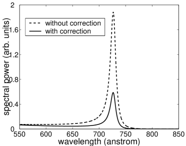
Figure 1: The profile of the spectral powers of Thosmon scattering with and without the correction, where $T_{e}=2$ keV, $n_{e}=2.1\times 10^{20}$ cm^-3, the probe wavelength is $0.5266$ $\mu$m and the scattering angle is $90^{\circ}$.

IV Plasma Dielectric Effect

When plasma density is high, the plasma dielectric effect may also be significant. In the case that the plasma dielectric effect cannot be neglected, the intensity of an electromagnetic wave in the plasma is given by

$$I=\frac{c}{8\pi}\sqrt{\epsilon(\omega_{0})}E^{2},$$

where $\epsilon(\omega)=1-\omega^{2}/\omega_{pe}^{2}$ is the plasma dielectric constant. And the differential wave vector also changes a little,

$$\mathbf{k}=\frac{\omega_{s}}{c}\sqrt{\epsilon(\omega_{s})}\mathbf{n}-\frac{\omega_{0}}{c}\sqrt{\epsilon(\omega_{0})}\mathbf{n}_{0}.$$ (31)

The scattering power is now given by

$$\frac{d^{2}P_{\mathbf{n}_{s},\omega_{s}}}{d\omega_{s}d\Omega}=r_{e}^{2}I_{0}N_{s}(\mathbf{e}_{0}\times\mathbf{n})^{2}\sqrt{\frac{\epsilon(\omega_{s})}{\epsilon(\omega_{0})}}S(k,\omega)\left(1+\frac{5\omega}{2\omega_{0}}\right).$$ (32)

Here, the plasma dielectric effect on the correction term is neglected.

We plot in Fig. 2 the profiles of the features of the scattering spectrum off an thermal electron plasma wave with and without the dielectric effect. As seen in Fig. 2, there is some differences when the dielectric effect is taken into account: the wavelength shift becomes smaller and the intensity becomes a little higher. The reason is quite understandable. When the dielectric effect is included, the differential wave vector becomes a little smaller, leading to a lighter damping and a lower frequency of the waves. That the factor $\sqrt{\epsilon(\omega_{s})/\epsilon(\omega_{0})}$ is larger than $1$ when $\omega<0$ also leads to a little higher intensity. The plasma dielectric effect becomes more notable when the plasma density is higher. In the case of $n_{e}/n_{c}$ is about several percent, the dielectric effect should be included in inferring the plasma parameters from the features of electron plasma waves.

The dielectric effect on the ion-acoustic features of Thomson scattering is much less significant. Since $\omega_{s}$ is very close to the probe frequency $\omega_{0}$ in this case, the dielectric effect just leads to a minor frequency shift $\delta\omega/\omega_{ia}\sim 0.5(n_{e}/n_{c})$, which is usually $\lesssim 10^{-2}$ in experiment. Therefore, the dielectric effect can be neglected in fitting the ion-acoustic feature of a Thomson spectrum.

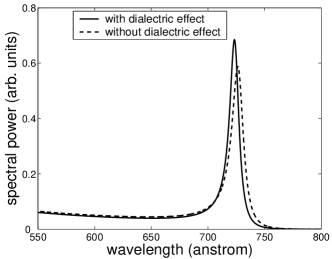
Figure 2: The profile of the spectral power of Thomson scattering with and without the plasma dielectric effect, where the parameters is the same with those used in Fig. 1

V Effect of finite scattering volume

When the scattering volume is small, the geometry factor may become important. When discussing the finite scattering volume effect, we neglect the correction terms in the first order of $v/c$. We then have

$$\frac{d^{2}P_{\mathbf{n}_{s},\omega_{s}}}{d\omega_{s}d\Omega}=n_{e}r_{e}^{2}I_{0}(\mathbf{e}_{0}\times\mathbf{n})^{2}\int\frac{d^{3}q}{(2\pi)^{3}}|G(\mathbf{q})|^{2}S(|\mathbf{k}-\mathbf{q}|,\omega)$$ (33)

In the case of $k\gg q$, we can approximately have

$$\frac{d^{2}P_{\mathbf{n}_{s},\omega_{s}}}{d\omega_{s}d\Omega} \approx n_{e}r_{e}^{2}I_{0}(\mathbf{e}_{0}\times\mathbf{n})^{2}\int\frac{d^{3}q}{(2\pi)^{3}}|G(\mathbf{q})|^{2}\left[S(k,\omega)-\mathbf{q}\cdot\frac{\partial}{\partial\mathbf{k}}S(k,\omega)\right]$$

$$\sim N_{s}r_{e}^{2}I_{0}(\mathbf{e}_{0}\times\mathbf{n})^{2}S(k,\omega)\left[1+\frac{\Delta q}{k}\right].$$

Hence $\Delta q$ is the range that $G(\mathbf{q})$ is notably different from zero. With the assumption that the scattering volume is a cubic with a length of $L$, $\Delta q\sim 2\pi/L$. Then the correction due to the finite scattering volume effect is about

$$\frac{\Delta q}{k}\sim\frac{2\pi}{kL}\sim\frac{\lambda_{0}}{2L\sin(\theta_{s}/2)},$$

where $\theta_{s}$ is the scattering angle and $\lambda_{0}$ is the probe wavelength. For a scattering experiment with a laser wavelength of $0.53$ $\mu$m and the scattering volume size of $50\times 50\times 50$ $\mu$m³ and scattering angle of $90^{\circ}$, this correction is about $10^{-2}$ and can be thereby neglected.

VI Summary

We revisit the theory of Thomson scattering from high-temperature high-density plasmas. Three effects are discussed: the correction due to finite $v/c$, the plasma dielectric effect, and the finite scattering volume effect. Among these three effects, the correction due to finite $v/c$ is the most important for analyzing the scattering spectrum off electron plasma waves. The plasma dielectric effect is less important but still notable. The finite scattering volume effect can be neglected if the size of the scattering volume is about $10^{2}$ of the probe wavelength and the scattering angle is not very small.

*

Appendix A

We first demonstrate that the normal dynamic form factor of a collisionless plasma can be obtained from Eq. (28) with the spectral density (26).

The electron susceptibility of a collisionless plasma is given by

$$\chi_{e}(k,\omega)=\frac{4\pi e^{2}}{m_{e}k^{2}}\int\frac{\mathbf{k}\cdot\partial f_{e}(\mathbf{v})/\partial\mathbf{v}}{\omega-\mathbf{k}\cdot\mathbf{v}+i0}d^{3}v.$$ (34)

When the distribution function of the electrons is Maxwellian,

$$f_{e}=\frac{n_{e}}{(2\pi)^{3/2}v_{e}^{3}}\exp\left(-\frac{v^{2}}{2v_{e}^{2}}\right),$$

the electron susceptibility can be written as

$$\chi_{e}=\frac{1}{k^{2}\lambda_{D}^{2}}\left[1+\frac{\omega}{\sqrt{2}kv_{e}}W\left(\frac{\omega}{\sqrt{2}kv_{e}}\right)\right],$$

where $W(x)$ is the plasma dispersion function. We further introduce the functions $F_{\alpha}$,

$$F_{\alpha}(\omega/k)=\int f_{\alpha}(\mathbf{v})\delta(\omega-\mathbf{k}\cdot\mathbf{v})d^{3}v=\frac{n_{\alpha}}{\sqrt{2\pi}kv_{\alpha}}\exp\left(-\frac{\omega^{2}}{2k^{2}v_{\alpha}^{2}}\right).$$

Then we have

$$\int d^{3}vd^{3}v^{\prime}2\pi\delta(\mathbf{v}-\mathbf{v}^{\prime})f_{e}(\mathbf{v})\delta(\omega-\mathbf{k}\cdot\mathbf{v})=2\pi F_{e}(\omega/k),$$

$$\int d^{3}vd^{3}v^{\prime}\frac{e^{2}(\mathbf{k}\cdot\partial f_{e}/\partial\mathbf{v})(\mathbf{k}\cdot\partial f_{e}/\partial\mathbf{v}^{\prime})}{m_{e}^{2}(\omega-\mathbf{k}\cdot\mathbf{v}+i0)(\omega-\mathbf{k}\cdot\mathbf{v}^{\prime}-i0)}\frac{32\pi^{3}}{k^{4}\left|\epsilon_{l}(\omega,k)\right|^{2}}\sum_{\alpha=e,i}e_{\alpha}^{2}\int f_{\alpha}(\mathbf{v})\delta(\omega-\mathbf{k}\cdot\mathbf{v})d^{3}v$$

$$=2\pi\left|\frac{\chi_{e}(\omega/k)}{\epsilon_{l}(\omega/k)}\right|^{2}\left[F_{e}(\omega/k)+Z^{2}F_{i}(\omega/k)\right],$$

$$-\frac{8\pi^{2}e^{2}}{k^{2}}\int d^{3}vd^{3}v^{\prime}\left\{\frac{[\mathbf{k}\cdot\partial f_{e}(\mathbf{v})/\partial\mathbf{v}]f_{e}(\mathbf{v}^{\prime})\delta(\omega-\mathbf{k}\cdot\mathbf{v}^{\prime})}{m_{e}\epsilon_{l}(\omega,k)(\omega-\mathbf{k}\cdot\mathbf{v}+i0)}+\frac{f_{e}(\mathbf{v})[\mathbf{k}\cdot\partial f_{e}(\mathbf{v}^{\prime})/\partial\mathbf{v}^{\prime}]\delta(\omega-\mathbf{k}\cdot\mathbf{v})}{m_{e}\epsilon_{l}^{\ast}(\omega,k)(\omega-\mathbf{k}\cdot\mathbf{v}^{\prime}-i0)}\right\}$$

$$=-2\pi\left[\frac{\chi_{e}}{\epsilon_{l}}+\frac{\chi_{e}^{\ast}}{\epsilon_{l}^{\ast}}\right]F_{e}(\omega/k),$$

Combining the above results, we have

$$\int d^{3}vd^{3}v^{\prime}(\delta f_{e}^{2})_{\omega,\mathbf{k},\mathbf{v},\mathbf{v}^{\prime}}=2\pi\left\{\left|\frac{1+\chi_{i}(\omega,k)}{\epsilon_{l}(\omega,k)}\right|^{2}F_{e}(\omega/k)+Z^{2}\left|\frac{\chi_{e}(\omega/k)}{\epsilon_{l}(\omega/k)}\right|^{2}F_{i}(\omega/k)\right\}.$$

Finally, we obtain the normal dynamic form factor,

$$S(k,\omega)=\frac{1}{\sqrt{2\pi}kv_{e}}\left|\frac{1+\chi_{i}(\omega,k)}{\epsilon_{l}(\omega,k)}\right|^{2}\exp\left(-\frac{\omega^{2}}{2k^{2}v_{e}^{2}}\right)+\frac{Z}{\sqrt{2\pi}kv_{i}}\left|\frac{\chi_{e}(\omega/k)}{\epsilon_{l}(\omega/k)}\right|^{2}\exp\left(-\frac{\omega^{2}}{2k^{2}v_{i}^{2}}\right).$$

Equation (27) is verified as follows. It is easy to demonstrate the following two equations,

$$\int\mathbf{v}f_{e}(\mathbf{v})\delta(\omega-\mathbf{k}\cdot\mathbf{v})d^{3}v=\frac{\mathbf{k}}{k}\frac{\omega}{k}F_{e}(\omega/k),$$

$$\int\frac{\mathbf{v}(\mathbf{k}\cdot\partial f_{e}/\partial\mathbf{v})}{\omega-\mathbf{k}\cdot\mathbf{v}+i0}d^{3}v=\frac{\mathbf{k}}{k}\frac{\omega}{k}\int\frac{\mathbf{v}(\mathbf{k}\cdot\partial f_{e}/\partial\mathbf{v})}{\omega-\mathbf{k}\cdot\mathbf{v}+i0}d^{3}v.$$

With aid of these two equations, we have

$$\frac{1}{2\pi n_{e}}\int\mathbf{v}(\delta f_{e}^{2})_{\omega,\mathbf{k},\mathbf{v},\mathbf{v}^{\prime}}d^{3}vd^{3}v^{\prime}=\frac{\mathbf{k}}{k}\frac{\omega}{k}S(k,\omega).$$

Then we obtain Eq. (27).

References

• (1) B. La Fontaine, H. A. Baldis, D. M. Villeneuve, J. Dunn, G. D. Enright, J. C. Kieffer, H. Pėpin, M. D. Rosen, D. L. Matthews, and S. Maxon, Phys. Plasmas 1, 2329 (1994).
• (2) S. H. Glenzer, C. A. Back, K. G. Estabrook, R. Wallace, K. Baker, B. J. MacGowan, B. A. Hammel, R. E. Cid, and J. S. De Groot, Phys. Rev. Lett. 77, 1496 (1996).
• (3) S. H. Glenzer, C. A. Back, L. J. Suter, M. A. Blain, O. L. Landen, J. D. Lindl, B. J. MacGowan, G. F. Stone, R. E. Turner, and B. H. Wilde, Thomson Scattering from Inertial-Confinement-Fusion Hohlraum Plasmas, Phys. Rev. Lett. 79, 1277 (1997).
• (4) S. H. Glenzer, W. Rozmus, B. J. MacGowan, K. G. Estabrook, J. D. De Groot, G. B. Zimmerman, H. A. Baldis, J. A. Harte, R. W. Lee, E. A. Williams, and B. G. Wilson, Phys. Rev. Lett. 82, 97 (1999).
• (5) B. Bai, J. Zheng, W. D. Liu, C. X. Yu, X. H. Jiang, X. D. Yuan, W. H. Li, and Z. J. Zheng, Phys. Plasmas 8, 4144 (2001).
• (6) Z. B. Wang, J. Zheng, B. Zhao, C. X. Yu, X. H. Jiang, W. H. Li, S. Y. Liu, Y. K. Ding, and Z. J. Zheng, Phys. Plasmas 12, 082703 (2005).
• (7) Q. Z. Yu, J. Zhang, Y. T. Li, X. Lu, J. Hawreliak, J. Wark, D. M. Chambers, Z. B. Wang, C. X. Yu, X. H. Jiang, W. H. Li, S. Y. Liu, and Z. J. Zheng, Phys. Rev. E. 71, 046407(2005).
• (8) D. H. Froula, P. Davis, L. Divol, J. S. Ross, N. Meezan, D. Price, and S. H. Glenzer, C. Rousseaux, Phys. Rev. Lett. 95, 195005 (2005).
• (9) D. H. Froula, J. S. Ross, B. B. Pollock, P. Davis, A. N. James, L. Divol, M. J. Edwards, A. A. Offenberger, D. Price, R. P. J. Town, G. R. Tynan, and S. H. Glenzer, Phys. Rev. Lett. 98, 135001 (2007).
• (10) J. Zheng, C. X. Yu, and Z. J. Zheng, Phys. Plasmas 4, 2736 (1997).
• (11) Z. J. Liu, J. Zheng, and C. X. Yu, Phys. Plasmas 9, 1073 (2002).
• (12) J. F. Myatt, W. Rozmus, V. Yu. Bychenkov, and V. T. Tikhonchuk, Phys. Rev. E 57, 3383 (1998).
• (13) J. Zheng, C. X. Yu, and Z. J. Zheng, Phys. Plasmas 6, 435 (1999).
• (14) W. Rozmus, S. H. Glenzer, K. G. Estabrook, H. A. Baldis, and B. J. MacGowan, Astrophys. J., Suppl. Ser. 127, 459 (2000).
• (15) Z. B. Wang, B. Zhao, J. Zheng, G. Y. Hu, W. D. Liu, C. X. Yu, X. H. Jiang, W. H. Li, S. Y. Liu, Y. K. Ding, and Z. J. Zheng, ACTA PHYSICA SINICA 54, 211 (2005) [in Chinese].
• (16) R. A. Pappert, Phys. Fluids 6, 1452 (1963).
• (17) R. E. Pechacek and A. W. Trivelpiece, Phys. Fluids 10, 1688 (1967).
• (18) A. G. Sitenko, Electromagnetic Fluctuations in Plasma (Academic Press, New York, 1967).
• (19) J. Sheffield, Plasma Scattering of Electromagnetic Radiation (Academic Press, New York, 1975).
• (20) L. D. Landau and E. M. Lifshitz, The Classical Theory of Fields (Pergoman, Oxford, 1975), 4th Edition.
• (21) E. M. Lifshitz and L. P. Pitaevskii, Physical Kinetics (Pergamon, Oxford, 1981).
• (22) D E Evans and J Katzenstein, Laser light scattering in laboratory plasmas, Rep. Prog. Phys. 32, 207 (1969).