Conductance through strongly interacting rings in a magnetic field

Abstract

We study the conductance through finite Aharonov-Bohm rings of interacting electrons weakly coupled to non-interacting leads at two arbitrary sites. This model can describe an array of quantum dots with a large charging energy compared to the interdot overlap. As a consequence of the spin-charge separation, which occurs in these highly correlated systems, the transmittance is shown to present pronounced dips for particular values of the magnetic flux piercing the ring. We analyze this effect by numerical and analytical means and show that the zero-temperature equilibrium conductance in fact presents these striking features which could be observed experimentally.

1 Introduction

One of the challenges of nanotechnology is the possibility of fabricating new artificial structures with tailored properties. For example, the Kondo effect was achieved in a system consisting of one quantum dot connected to leads[1, 2, 3]; systems of a few QD’s have been proposed theoretically as realizations of the two-channel Kondo model [4, 5], the ionic Hubbard model, [6] and the double exchange mechanism. [7] Also, the correlation-driven metal-insulator transition has been studied in a chain of quantum dots. [8]

Another interesting phenomenon in strongly correlated systems is what is known as charge-spin separation. It is well known that strong correlations in one dimension invalidate the Fermi liquid conventional description of electrons. In particular, correlations can lead to the fractionalization of the electron into charge and spin degrees of freedom.[9] This separation is an asymptotic low-energy property in an infinite chain. However, exact Bethe ansatz results for the Hubbard model in the limit of infinite Coulomb repulsion $U$ show that the wave function factorizes into a charge and a spin part for any size of the system. [10] There have been several experiments reporting indirect indications of charge-spin separation  [11, 12, 13], and it could also be potentially observed in systems such as cuprate chains, ladder compounds, [14] and carbon nanotubes. [15]

Several theoretical approaches tackled this phenomenon in the ring geometry. For example, the real-time evolution of electronic wave packets in Hubbard rings has shown a splitting in the dispersion of the spin and charge densities as a consequence of the different charge and spin velocities. [16, 17] Pseudospin-charge separation has also been studied in quasi-one-dimensional quantum gases of fermionic atoms. [18, 19] Other theoretical approaches concern the transmittance through Aharonov-Bohm rings modeled by Tomonaga-Luttinger liquid or other correlated Hamiltonians like the Hubbard or $t-J$ models.[20, 21, 22, 23] In these systems, noticeable dips are observed in the conductance for fractional values of the flux which can be attributed to destructive interference between degenerate states as we explain below. We have recently discussed the extension of these results to ladders of two legs as a first step to higher dimensions. [24]

In this work, we analyze the origin of the dips in the transmittance as a function of applied flux in finite rings described by the $t-J$ model. We discuss the conditions for which the intensity of the lowest-lying peak in the zero-temperature equilibrium conductance as a function of the gate voltage presents characteristic dips for certain flux values. These will be shown to be a consequence of spin-charge separation.

2 Model Hamiltonian

The basic model is depicted in Fig. 1. We have considered a ring of $L$ sites, weakly connected to non-interacting leads at sites $0$ and $M$.

Figure 1: Schematic representation of the systems studied numerically. (a) $L=6$, (b) $L=7$. In both cases $M=3$.

The Hamiltonian reads:

$$H=H_{\mathrm{ring}}+H_{\mathrm{leads}}+H_{\mathrm{links}}.$$ (1)

The first term describes the isolated ring, with on-site energy given by a gate voltage $V_{g}$, and hoppings modified by the phase $\exp(i\phi/L)$ due to the circulation of the vector potential. For most of the results of this paper we use the $t-J$ model to describe the ring,

$$H_{\mathrm{ring}} = -eV_{g}\sum_{i\sigma}c_{i\sigma}^{{\dagger}}c_{i\sigma}-t\left(c_{i+1\sigma}^{{\dagger}}c_{i\sigma}e^{i\phi/L}+\mathrm{H.c.}\right)$$ (2)

$$+J\sum_{i}\left(\mathbf{S}_{i}\cdot\mathbf{S}_{i+1}-\frac{1}{4}\right).$$

where $\phi=2\pi\Phi/\Phi_{0}$, $/\Phi_{0}=h/2e$ is the flux quantum, $\mathbf{S}_{i}$ is the spin operator at site $i$ and double occupancy is not allowed at any site of the ring. The second term corresponds to two tight-binding semi-infinite chains for the left and right leads

$$H_{\mathrm{leads}}\!=\!-t\!\!\!\sum_{i=-\infty,\sigma}^{-1}\!\!\!a_{i-1,\sigma}^{{\dagger}}a_{i,\sigma}\!-t\!\!\!\sum_{i=1,\sigma}^{\infty}\!a_{i,\sigma}^{{\dagger}}a_{i+1,\sigma}\!+\!\mathrm{H.c.}$$ (3)

The third term in Eq. (1) describes the coupling of the left (right) lead with site 0 ($M$) of the ring

$$H_{\mathrm{links}}=-t^{\prime}\sum_{\sigma}(a_{-1,\sigma}^{{\dagger}}c_{0\sigma}+a_{1,\sigma}^{{\dagger}}c_{M\sigma}+\mathrm{H.c.}).$$ (4)

3 Conductance

When the ground state of the isolated ring is non-degenerate, and the coupling $t^{\prime}$ between the leads and ring is weak, the equilibrium conductance at zero temperature can be expressed to second order in $t^{\prime}$ in terms of the retarded Green’s function for the isolated ring between sites $i$ and $j$: $G_{i,j}^{\mathrm{R}}(\omega)$. [6, 20] For an incident particle with energy $\omega=-2t\cos k$ and momentum $\pm k$, the transmittance reads

$$T(\omega,V_{g},\phi)=\frac{4t^{2}\sin^{2}k|{\tilde{t}}(\omega)|^{2}}{\left|[\omega-{\epsilon}(\omega)+te^{ik}]^{2}-|{\tilde{t}}^{2}(\omega)|\right|^{2}},$$ (5)

where $\epsilon(\omega)=t^{\prime\,2}G_{00}^{\mathrm{R}}(\omega)$ and $\tilde{t}(\omega)=t^{\prime\,2}G_{0M}^{\mathrm{R}}(\omega)$ represent a correction to the on-site energy at the extremes of the leads and an effective hopping between them respectively.

This equation is in fact exact for a non-interacting system, however, it loses validity for an odd number of electrons, where the ground state is Kramers degenerate. In this case the method misses completely the interesting physics arising from the Kondo effect. [6, 25] However, the Kondo temperature is small compared to the other energy scales of the system and we can assume safely that the Kondo effect is destroyed by a small temperature. This approach is justified for small enough $t^{\prime}$ since the characteristic energy of this Kondo effect decreases exponentially.

The conductance is $G=(ne^{2}/h)T(\mu,V_{g},\phi)$, where $n=1$ or 2 depending if the spin degeneracy is broken or not, [6] and $\mu$ is the Fermi level, which we set as zero (half-filled leads). When the gate voltage $V_{g}$ is varied a peak in the conductance is obtained when there is a degeneracy in the ground state of the ring for two consecutive number of particles: $E_{g}(N+1)=E_{g}(N)$, where $E_{g}(N)$ is the ground state energy of $H_{\mathrm{ring}}$ with $N$ electrons. Without loss of generality, we assume that we start with $N+1$ electrons in the ring and apply a negative gate voltage in such a way that a peak in the conductance is obtained at a critical value $V_{g}^{c}$ when the number of electrons in the ring changes from $N+1$ to $N$ electrons.

4 Analytical and numerical results

For $J=0$ the model is equivalent to the Hubbard model with infinite on-site repulsion $U$, for which the wave function can be factorized into a spin and a charge part, evidencing charge-spin separation. [10, 22, 26] For each spin state, the system can be mapped into a spinless model with an effective flux which depends on the total spin. For a system of $N$ particles one can construct spin-wave functions with wave vectors $k_{s}=2\pi n_{s}/N$, where the integer $n_{s}$ characterizes the spin wave function. The total energy and momentum (in an appropriate gauge) of any state of the ring have simple expressions:

$$E = -2t\sum_{l=1}^{N}\cos(k_{l}),\;\;k_{l}=\frac{2\pi n_{l}+\phi_{\mathrm{eff}}}{L},$$ (6)

$$K = \sum k_{l}=\left[2\pi(n_{c}+n_{s})+N\phi\right]/L,$$ (7)

$$\phi_{\mathrm{eff}} = \phi+k_{s}=\phi+\frac{2\pi}{N}n_{s},$$ (8)

where the integers $n_{l}$ characterize the charge part of the wave function and $n_{c}=\sum n_{l}$.

The values of the flux $\phi_{d}$ for which dips or reduced conductances are expected, correspond to some particular crossings of the energy levels of $N$ electrons. One can see this from the general form of the Green’s functions $G_{0j}^{\mathrm{R}}(\omega)$ entering the transmittance [Eq. (5)] when a particle is destroyed. Using the Lehman’s representation, the relevant part of the Green’s function is:

$$G_{0j}^{\mathrm{R}}(\omega)=\sum_{e}\frac{\langle g|c_{j\sigma}^{\dagger}|e\rangle\langle e|c_{0\sigma}|g\rangle}{\omega+E_{e}-E_{g}}.$$ (9)

Noting that the ring has translational symmetry and naming $K_{\nu}$ the wave vector of the state $|\nu\rangle$, one obtains:

$$G_{0j}^{\mathrm{R}}(\omega)=\sum_{e}\frac{e^{-ij(K_{e}-K_{g})}|\langle e|c_{0\sigma}|g\rangle|^{2}}{\omega+E_{e}-E_{g}}.$$ (10)

At certain flux values, two states of $N$ electrons, $|e\rangle$ and $|e^{\prime}\rangle$, become degenerate. Assuming that the corresponding matrix elements entering Eq. (10) are nonzero, only these two states, contribute significantly to the Green’s function $G_{0j}^{\mathrm{R}}(\omega)$ at the Fermi energy ($\omega=\mu=0$) when $V_{g}$ (which displaces all $E_{e}$ rigidly with respect to $E_{g}$) is tuned in such a way that $E_{e}=E_{e^{\prime}}\sim E_{g}$. Denoting by $\beta=\exp[iM(K_{e^{\prime}}-K_{e})]$ the relative phase between the two intervening degenerate states we see that if $\beta\neq 1$, the transmittance, which is proportional to $|G_{0M}^{\mathrm{R}}(\omega)|^{2}$, (Eq. (5)), is reduced near the crossing (note that this results is independent of any specific model).

We can predict the positions of the dips in the transmittance without having to resort to the calculation of the matrix elements entering the Green s functions Eq. (10). The crossings of energy levels at low energies take place at $\phi=-\pi(n_{s}+n_{s}^{\prime})/N$.[23] When $n_{s}+n_{s}^{\prime}$ is odd (even) the relative phase $\beta=\exp[iL(K_{e^{\prime}}-K_{e})/2]=\exp\left[i(n_{s}^{\prime}-n_{s})\right]$  $=-1$ (1) and there is (there is not) a dip in the integrated transmittance. Therefore, the positions of the dips are located at

$$\phi_{d}=\pi(2n+1)/N,$$ (11)

with $n$ integer. These are also the positions where crossings in the (experimentally accessible) ground state for $N$ particles take place ($n_{s}^{\prime}-n_{s}=\pm 1$).

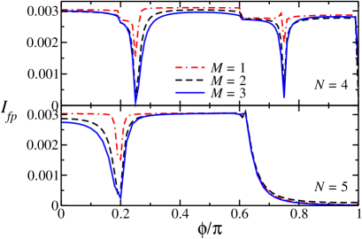
Figure 2: Intensity of the first peak in the transmittance $I_{fp}$, as a function of applied magnetic flux, for a ring of 6 sites and (a) $N+1=5$ and (b) $N+1=6$ electrons in the ground state, three different configurations $M=1$, 2 and 3, $t^{\prime}=0.3t$ and $J=0.001t$.

To check these predictions we have performed numerical calculations for the transmittance, obtained by diagonalizing the ring using Davidson’s method [27]. Once the Green’s functions were obtained, they were replaced in Eq. (5), to obtain the transmittance. The systems studied are represented in Fig. 1. In contrast to previous work, [20, 21, 22, 24] we concentrate on the first peak in the transmittance as the gate voltage is decreased since this is the feature which is experimentally accessible at equilibrium and low temperatures.

In Fig. 2 we show numerical results for a ring with $L=6$ sites and $N=4$ and 5 particles in the intermediate state for the three non-equivalent configurations corresponding to $M=1$, 2 and 3. To quantify the relative intensity of the conductance we integrate the transmittance given by Eq. (5) over a window of gate voltage $V_{g}$ of width $0.002t$ centered around the degeneracy point between the ground state for $N+1$ and $N$ electrons. This corresponds to the intensity of the first observable peak in the transmittance as the gate voltage is lowered. As the curve is symmetric under change of sign of $\phi$ we show only the interval $0\leq\phi\leq\pi$. For $J\rightarrow 0$ and $N=4$ the dips appear as expected (Eq. (11)) at $\phi_{d}/\pi=0.25$ and 0.75. For $N=5$ the dips should occur at $\phi_{d}/\pi=0.2$, 0.6 and 1. However, near 0.6 the total spin in the ground state for 5 electrons changes from $S=1/2$ to $S=3/2$, which is not accessible by destroying an electron in the 6-electron singlet ground state. Therefore, the transmittance vanishes for $0.6<\phi\leq\pi$. As a consequence, in the interval shown there is only one dip present. In this figure one can see the effect of the different source-drain configurations: the lowest conductance is achieved for the symmetric case ($M=3$ for $L=6$) where $\beta=-1$ and both degenerate levels interfere destructively. For the other cases the interference is less destructive and a less pronounced dip is obtained.

It is also interesting to analyze the conductance for different particle numbers to study the evolution of the dips as predicted in Eq. (11). This is shown in Fig. 3. The number of particles in the intermediate situation, $N$, is shown for each case. Here we see that the minima do in fact occur for the fluxes predicted by that relation very accurately. The abrupt step obtained for $N=2$ corresponds, again, to a forbidden transition to a large total spin state from a singlet ground state as explained above.

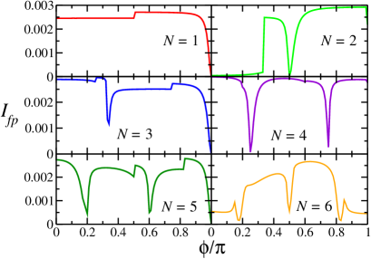
Figure 3: Intensity of the first peak in the transmittance $I_{fp}$, as a function of applied magnetic flux, for a ring of 7 sites and several fillings. Here $M=3$, $t^{\prime}=0.3t$ and $J=0.001t$.

5 Conclusions

We have presented results for the zero-temperature equilibrium conductance through finite rings described by the $t-J$ model threaded by a magnetic flux, weakly coupled to conducting leads. At particular values of the flux we find dips or reductions of the transmittance, which are due to negative interferences between degenerate levels. This can be understood by analyzing the extremely interacting case for $J=0$, where exact results are available. The position of the dips reflect the particular features of the spectrum in this limit, in which the charge and spin degrees of freedom are separated at all energies. For finite $J$ the positions of the dips change and some additional dips can also appear in a manner that is difficult to predict and which is not yet fully understood.

The negative interference depends on the source-drain configuration. It is more marked if the leads are connected at angles near 180 degrees. These results are confirmed by our numerical calculations.

References

- [1] D. Goldhaber-Gordon et al., Nature 391, 156 (1998).
- [2] S. M. Cronenwet, T. H. Oosterkamp, and L. P. Kouwenhoven, Science 281, 540 (1998).
- [3] W.G. van der Wiel, et al., Science 289, 2105 (2000).
- [4] Y. Oreg and D. Goldhaber-Gordon, Phys. Rev. Lett. 90, 136602 (2003).
- [5] R. Žitko and J. Bonča, Phys. Rev. B 74, 224411 (2006).
- [6] A. A. Aligia, K. Hallberg, B. Normand, and A. P. Kampf, Phys. Rev. Lett. 93, 076801 (2004).
- [7] G. B. Martins et al., Phys. Rev. Lett. 94, 026804 (2005).
- [8] L. P. Kouwenhoven et al., Phys. Rev. Lett. 65, 361 (1990).
- [9] T. Giamarchi, Quantum physics in one dimension (Clarendon Press, Oxford, 2004).
- [10] M. Ogata and H. Shiba, Phys. Rev. B 41, 2326 (1990).
- [11] J. Voit, Rep. Prog. Phys. 58, 977 (1995).
- [12] C. Kim et al., Phys. Rev. Lett. 77, 4054 (1996).
- [13] Q. Si, Phys. Rev. Lett. 78, 1767 (1997); Physica C 341, 1519 (2000).
- [14] E. Dagotto and T. M. Rice, Science 271, 618 (1996).
- [15] A. De Martino, R. Egger, K. Hallberg and C.A. Balseiro, Phys. Rev. Lett. 88, 206402 (2002)
- [16] E. A. Jagla, K. Hallberg, and C. A. Balseiro, Phys. Rev. B 47, 5849 (1993).
- [17] C. Kollath, U. Schollwöck and W. Zwerger, Phys. Rev. Lett. 95, 176401 (2005)
- [18] A. Recati et al., Phys. Rev. Lett. 90, 020401 (2002)
- [19] L. Kecke, H. Grabert, and W. Hausler, Phys. Rev. Lett. 95, 176802 (2005)
- [20] E. A. Jagla and C. A. Balseiro, Phys. Rev. Lett. 70, 639 (1993)
- [21] S. Friederich and V. Meden, Phys. Rev. B 77, 195122 (2008).
- [22] K. Hallberg, A. A. Aligia, A. Kampf and B. Normand, Phys. Rev. Lett. 93, 067203 (2004).
- [23] J. Rincón, A. A. Aligia, K. Hallberg, Phys. Rev. B, in press (2008).
- [24] J. Rincón, K. Hallberg and A. A. Aligia, Phys. Rev. B 78, 125115 (2008)
- [25] A. M. Lobos and A. A. Aligia, Phys. Rev. Lett. 100, 016803 (2008)
- [26] W. Caspers and P. Ilske, Physica A 157, 1033 (1989); A. Schadschneider, Phys. Rev. B 51, 10386 (1995).
- [27] E. R. Davidson, J. Comput. Phys. 17, 87 (1975); Comput. Phys. Comm. 53, 49 (1989)