Statistical description of domains in the Potts model

Abstract

The Zipf power law and its connection with the inhomogeneity of the system is investigated. We describe the statistical distributions of the domain masses in the Potts model near the temperature-induced phase transition. We found that the statistical distribution near the critical point is described by the power law form with a long tail, while beyond the critical point the power law tail is suppressed.

We use the Potts model [1] for the description of the phase transition. The Potts model is the generalization of the Ising model with more than two spin components and it has more experimental realizations than the Ising model. For a detailed review of Potts model see [2].

The Hamiltonian for the $q-$state Potts model [2] is:

$$H=-\sum\limits_{ij}J_{ij}\delta_{\sigma_{i},\sigma_{j}},$$ (1)

where $\sigma_{i}\in\{1,2,...,q\},$ $\delta_{x,y}$ is the Kronecker delta

$$\delta_{x,y}=\left\{\begin{array}[]{l}1\quad\mbox{if \ $x=y$,}\\[5.69054pt] 0\quad\mbox{otherwise}.\end{array}\right.$$

and

$$J_{ij}=\left\{\begin{array}[]{l}J\quad\mbox{if \ $i,j$ are neighbour pairs of spins,}\\[5.69054pt] 0\quad\mbox{in opposite case}.\end{array}\right.$$

The case $q=2$ describes the Ising model.

The results presented hereafter are obtained by applying the Monte Carlo techniques, based on the Metropolis algorithm [3], to the two-dimensional $q-$state Potts model with the periodic boundary conditions and with $q=3$ and $6$.

A number of exact results for the two -dimensional Potts models are known in the infinite volume limit. For example, the phase transition appears at the critical temperature $\,T=T_{c}\,$ ($\,T_{c}=2J/k_{B}\,\ln(1+\sqrt{q})\,$). It is the second order phase transition for $q\leq 4$ and the first order one for $q\geq 5$, see [4] and [2].

The main goal of this paper is the statistical description of the domains in Potts model when one approaches the critical point of the phase transition induced by the temperature. This problem has been investigated for the Ising model in [5]. Our considerations concerning the statistical description of domain masses have universal character and may be used to arbitrary fractal system of elements which are described by the random variables $x$. This variables can be listed in the decreasing order. For example: the rank of the city connected with its population, the frequency of the occurrence of any word in the text, the trading value of largest European’s companies or the hyperbolic processes in finance [6], [7].
We consider the Zipf power law [8] in Bouchaud notation [6]:

$$x=k^{-\frac{1}{\mu}}$$ (2)

This law is used often in the description of self-organized critical phenomena.

In our case $\,x\,$ is the number of the Potts spins in the domain called the domain mass and $\,k\,$ denotes the rank of the domain mass $\,x$.The geometrical clusters are considered [9]. The greatest cluster has the rank 1, smaller 2 and so on. In the Potts model, clusters are sets of nearest neighbour sites occupied by Potts spins with the same orientation. For a given configuration of spins clusters are determined uniquely. There is the well establish connection between thermal and geometric phase transitions. In the dimension two an infinite cluster appears exactly at the critical point. The $q-$state Potts model has the ground state degeneracy $q$ and after a quench from the high-temperature phase, small domains start to grow, thus reducing the domain boundary curvature. One can notice that there is a difference between the domains of the Potts model with $q=2$ (the Ising model case) and the Potts model with $q>2$. For $q=2$ the domain boundaries are represented by long filaments of one phase within the other one, whereas for $q>2$, the domains resemble the structure characteristic for polycrystalline grains [10], [11] and [12] - i.e. the boundaries are straight and meet at fixed angles.

We take into account, in our considerations, all domains and we concentrate on their size. Bouchaud [6] pointed out the strong correlation between the Zipf power law and the inhomogeneity of the system. We are going to test the log-log distribution of domain masses versus the rank index $k$ when we come near the critical point in the temperature-induced phase transition.

The slope $\alpha$ of the regression line describing relation between the logarithm of the cluster mass and the logarithm of its rank is given by$\mu$ $(-\frac{1}{\mu}={\rm tg}\,\alpha)$, and it characterizes the inhomogeneity of the physical structure of the system. The inhomogeneity of the system means that its structure has become fractal and more hierarchical. We expect that $\mu$ value will depend on whether we are far or close to the critical point. In particular one should have $\mu\approx 1$ in the critical point and $\mu>1$ beyond the criticality. This follows from the following considerations. It is shown in [13] that there is a conjecture between Zipf exponent and the Hurst exponent $H$ [14] of the form

$$1/\mu=|2H-1|$$ (3)

It is well known that any complex system exhibits long-range (infinite-long) correlations at the critical point. This corresponds to the biggest value of Hurst exponent, i.e. $H=1$. In such a case one obtains from Eq.(3) $\mu\approx 1$.
The criticality in the rank statistics was also considered experimentally in [15],[16] investigating distributions of island areas of discontinuous metal films near the percolation threshold.
In our consideration we shall concentrate on random variable $X$ which we shall call $\,[\mu]-variable.$ We say that the random variable $X$ is $[\mu]-variable$ if for some $x_{0}>0$ and $\mu>0,$ a tail of its distribution function decays as $\left(\frac{x_{0}}{x}\right)^{\mu}.$

The main property of $\,[\mu]-variable$ is that all its moments $\,m_{q}=<x^{q}>\,$ with $\,q\geq\mu\,$ are infinite. The distribution of the cluster size seems to be $[\mu]$-distribution and the index $\mu$ is a critical exponent.

The simplest technique which helps to test heavy tail hypothesis and estimates the tail index $\mu$ is based on the following reasoning, (for more details see [17]).

Let $X_{1},\,X_{2},\,...,\,X_{n}$ be independent and identically distributed random variables with distribution function $F$. We may re-arrange the $X_{i}$ in the decreasing order. Denoting the largest value, with rank 1, by $X_{(1)},$ the next largest, with rank 2, by $X_{(2)}$ etc., we arrive at the sequence of order statistics

$$X_{(1)}\geq X_{(2)}\geq\,...\geq X_{(n)}.$$

Assume that $X$ is a $\,[\mu]-variable$ with tail of its distribution function satisfying for some $x_{0}>0$ and $\mu>0$

$$P(X>x)=\left(\frac{x_{0}}{x}\right)^{\mu},\quad x>x_{0}.$$ (4)

The assumption (4) means that the distribution function of $\frac{X}{x_{0}}$ is the Pareto distribution with the left endpoint 1 and the parameter $\mu$, and for $x>0$

$$P\left(\mu\ln\frac{X}{x_{0}}>x\right)=\exp(-x)$$

which means that the distribution function of the random variable $\mu\ln\frac{X}{x_{0}}$ is exponential with parameter 1.

Therefore

$$P(\ln\,X>x)=\exp\left(-\frac{x-\ln x_{0}}{\mu^{-1}}\right),$$

which is a tail of shifted by $\ln x_{0}$ and rescaled by $\mu^{-1}$ exponential distribution function with parameter 1.

Drawing the quantile to quantile plot for the exponential distribution function we conclude that

$$\left\{\left(-\ln\left(\frac{i}{n+1}\right),\,\ln X_{(i)}\right),\,1\leq i\leq n\right\},$$

should be linear with slope $\mu^{-1}$ and intercept $\ln x_{0}$. In this way we obtain the Zipf power law. We may estimate $\mu$ in a different way. The most popular estimator of $\mu$ is the Hill estimator, [18]. For the convenience of the reader we recall its definition. The Hill’s estimator of $\frac{1}{\mu}$ based on $m$ upper-ordered statistics $X_{(1)}\geq X_{(2)}\geq...\geq X_{(m)}$ is defined as

$$H_{m,n}=\frac{1}{m}\sum_{i=1}^{m}\log\frac{X_{(i)}}{X_{(m+1)}}.$$ (5)

Our simulations were performed on two dimensional lattices $600\times 600$ with periodic boundary conditions. We used the Metropolis algorithm [3]. All simulations were initiated with the random initial orientation of spins. We thermalized the system to equilibrate the orientations of spins. The number of Monte Carlo steps which are necessary to reach the equilibrium state was chosen by measuring the average energy of one spin.

We performed 1 000 000 Monte Carlo steps to equilibrate the system. Once the equilibrium of the system is reached we took sample of the cluster configuration. Then we studied the distribution of the cluster masses. The total mass of the cluster was defined as the number of spins in the cluster.

Our aim is to connect the statistics of domain masses with the way the critical point is reached. When we start to advance from the paramagnetic phase to the critical point $\,(T\rightarrow T_{c})\,$ (as it is seen in Fig. 1, for $q=3$, and Fig. 2 for $q=6$) the slope of straight lines representing (in log-log scale) the Zipf power law increases when $\mu>1$.

Figure 1: The log-log distribution of the domain masses $x_{k}$ versus the rank order index $k$ for the 3-state Potts model for $\beta=0.40$ ($\Diamond$), $0.45$ ($\ast$), $0.49$ ($\Box$) and critical $\beta$ ($\circ$), for one configuration. The straight line are with the slopes $-1/\mu$ given in Table 1.

Figure 2: The log-log distribution of the domain masses $x_{k}$ versus the rank order index $k$ for the 6-state Potts model for $\beta=0.50$ ($\Diamond$), $0.55$ ($\ast$), $0.59$ ($\Box$) and critical $\beta$ ($\circ$), for one configuration. The straight line are with the slopes $-1/\mu$ given in Table 2.

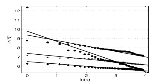
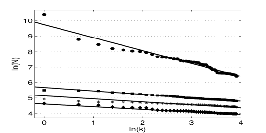
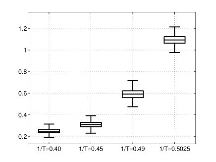
The estimations of indexes $\frac{1}{\mu}$, for the 3-state Potts model with different inverse temperature $\beta=1/T$, based on 1000 realizations for $600\times 600$ lattice are presented in Table 1 and Fig.3.

Figure 3: Box plot: The mean value of $\mu^{-1}$ (–) with standard deviation and 95% confidence interval, for inverse temperatures $\beta=0.40,0.45,0.49$ and and close to critical $0.50253$, obtained by averaging of 1000 Monte Carlo realizations of the 3-state Potts model on $600\times 600$ lattice.

The same estimations of indexes $\frac{1}{\mu}$ and its standard deviations as in Table 1 and Fig 3, but for 6-state Potts model, are presented in Table 2 and Fig.4.

Table 2. The estimation of index $\frac{1}{\mu}$ with standard deviation $s$.

$\beta$	$\mu^{-1}$	$s$
$0.50$	$0.172505$	$0.017357$
$0.55$	$0.193189$	$0.020260$
$0.59$	$0.219017$	$0.022300$
$\beta_{kr}\simeq 0.6191\quad$	$0.834464$	$0.043940$

Figure 4: Box plot: The mean value of $\mu^{-1}$ (–) with standard deviation and 95% confidence interval, for inverse temperatures $\beta=0.50,0.55,0.59$ and close to critical $0.6191$, obtained by averaging of 1000 Monte Carlo realizations of the 6-state Potts model on $600\times 600$ lattice.

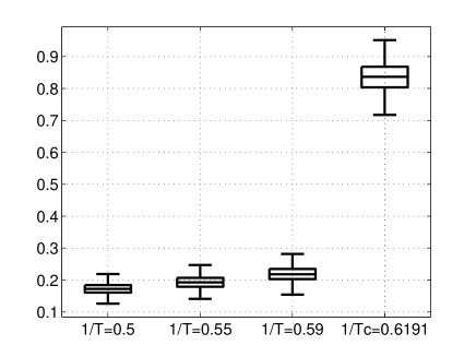
Fig. 5 and Fig. 6 represent the dependence between the number of domains with mass x normalized by number of configurations and mass(x) for 3-state and 6-state Potts models respectively, near the critical point. The distribution of domain mass is $F[\mu]$-distribution with $\mu\approx 1$ ,which means that it satisfies power law with a long tail: $\frac{x_{0}^{\mu}}{x^{1+\mu}}$,where $x_{0}$ denotes a typical scale and $\mu\simeq 1$.

Figure 5: The dependence between the number of domains with mass x normalized by number of configurations $(N_{x}/N)$ and the mass $(x)$ in the log-log scale for the 3-state Potts model near the critical point $T_{c}$ for 5000 configurations and $L=600$.

Figure 6: The dependence between the number of domains with mass x normalized by number of configurations $(N_{x}/N)$ and the mass $(x)$ in the log-log scale for the 6-state Potts model near the critical point $T_{c}$ for 5000 configuration and $L=600$.

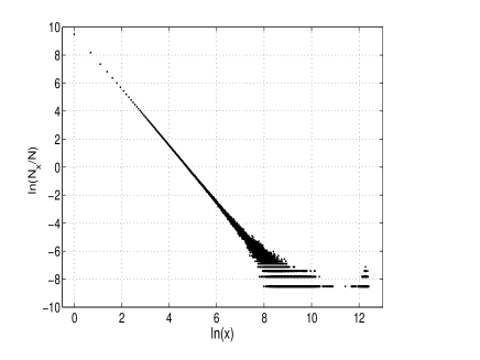
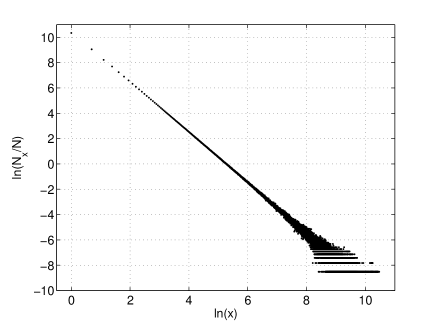
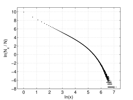
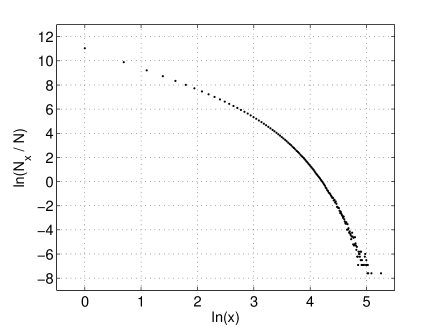
Fig. 7 and Fig. 8 represent the dependence between the number of domains with mass x normalized by number of configurations $(N_{x}/N)$ and the mass $(x)$ of domain masses for 3-state and 6-state Potts models beyond the critical region when $\mu>1$, respectively. In this case the distribution of domain masses is without heavy power-law tail. This results are in the agreement with the standard percolation theory [9].

Figure 7: The dependence between the number of domains with mass x normalized by number of configurations $(N_{x}/N)$ and the mass $(x)$ in the log-log scale for the 3-state Potts model for $\beta=0.4$ for 2000 configurations and $L=600$.

Figure 8: The dependence between the number of domains with mass x normalized by number of configurations $(N_{x}/N)$ and the mass $(x)$ in the log-log scale for the 6-state Potts model for $\beta=0.5$ for 2000 configuration and $L=600$.

The numerical results presented in Figures 5-8, usually can be deduced from the standard percolation theory [9] and are in the agreement with the previous results of [19] and [20]. The origin of the power-law is well understood and explained as a consequence of the scale invariance at the criticality regime due to the divergence of the correlation length. Beyond the criticality range, where the system is a fractal its correlation length is finite so the power-law tail in the distribution is suppressed. One of the possible experimental confirmations of the Zipf power law is the distribution of island areas of discontinuous metal films, obtained by evaporation of dielectric substances [15], [16]. Another one is the distribution of local fields intensities [21]. Unfortunately, the results of analogous experiment on ferromagnetic are not known.

The main result of our paper is obtained by applying the Zipf power law to the criticality region and beyond it for the phase transition in the Potts model.

Further, we have shown, by the simulation results, that the exponent in the Zipf power law describes the long tail behaviour of the distribution of domains masses at the critical point when $\mu\approx 1$.

These results deal with the physical phenomena different from those considered e.g., in [15], [16] and [21]. However in all cases the formulas describing properties of the system are similar and they are based on the Zipf power law. The statistical description gives the opportunity to test the phase transition not only in the critical region but also beyond the criticality.

Acknowledgments. One of the author (K. L-W) would like to express her gratitude to dr Dariusz Grech for the interest in this paper and valuable comments.

References

-
[1]
R. B. Potts, Ph. D. Thesis, University of Oxford (1951),
Proc. Camb. Phil. Soc. 48 (1952) 106. - [2] F. Y. Wu, Rev. Mod. Phys. 54 (182) 235.
- [3] N. Metropolis, A. W. Rosenbluth, M. N. Rosenbluth, A. H. Teller, E. Teller, J. Chem. Phys. 21 (1953) 1087.
- [4] R. J. Baxter, J. Phys. C 8 (1973) L445.
- [5] K. Lukierska-Walasek, K. Topolski, Preprint arXiv: cond-mat.stat-mech 0804.3522v1.
- [6] J.P. Bouchand, Proc. Int. Workshop on Lévy Flights and Related Topics in Physics (Nice, France, 27–30 June 1994) ed. by M.F. Shlesinger, G.M. Zasławsky, V. Frisch, Berlin, Springer, 1995.
- [7] M. Bibby, M. Sorensen, Handbook of Heavy Tailed Distributions in Finance Vol. 1 ed. S. T. Rachev, Elsevier (2003).
- [8] Human Behavior and the Principle of Least Effort (Addison-Wesley, New York, 1949).
- [9] D. Stauffer, A. Aharony Introduction to percolation theory, Taylor and Francis, London and Philadelphia, 1994.
- [10] J. M. Lifshitz, Sov. Phys. JETP 15 (1962) 939.
- [11] G. S. Grest, M.P. Anderson and J.P. Srolovitz, Phys. Rev. B 38 (1988) 4752.
- [12] M. R. Dudek, J. F. Grouyet, M. Kolb, Surface Science 401 (1998) 220.
- [13] A. Czirok, R.Mantegna, S. Havlin, H. E. Stanley, Phys. Rev. E.52 (1995) 446.
- [14] H. E. Hurst, Trans. Am. Soc. Civ. Eng. 116 (1951) 770
- [15] E. Dobierzewska-Mozrzymas, P. Bieganski, E. Piecul and J. Wojcik, J. Phys. Condens Matter 11 (1999) 5561.
- [16] E.Dobierzewska-Mozrzymas,G.Szymczak,P.Biega ski,E.Piecul,Physica B337(2003)79,
[17]
M. Kratz, S.I. Resnick, Stochastic Models, 12 (1996) 699.
J.Beirlant, Y. Goegebeeur, J. Teugels and J. Segers, Statistics of Extremes, Theory and Applications, Wiley, Chichester, UK, 2004. - [18] B. M. Hill, Ann. Stat. 3 (1975) 1163.
- [19] W. Janke and A. M. J. Schakel, Phys. Rev. E 71 (2005) 036703.
- [20] W. Janke and A. M. J. Schakel, Braz. J. Phys. 36 (2006) 708.
- [21] S. Liberman, F. Browers, P. Gadenne, Physica B 279 (2000) 56.