Vacuumless topological defects in Lyra geometry

Abstract

Few years ago, Cho and Vilenkin have proposed that topological defects can arise in symmetry breaking models without having degenerate vacua. These types of defects are known as vacuumless defects. In the present work, the gravitational field of a vacuumless global string and global monopole have been investigated in the context of Lyra geometry. We find the metric of the vacuumless global string and global monopole in the weak field approximations. It has been shown that the vacuumless global string can have repulsive whereas global monopole exerts attractive gravitational effects on a test particle. It is dissimilar to the case studied in general relativity.

Introduction:

Topological defects such as domain walls, monopoles and cosmic strings could be produced at a phase transition in the early Universe [1]. Their nature depends on the symmetry breaking in the field theory under consideration. In Cosmology, these defects have been put forward as a possible source for the density perturbations which seeded the galaxy formation.
The Lagrangian of a typical symmetry breaking model is of the form

$$L=\frac{1}{2}\partial_{\mu}\Phi^{a}\partial^{\mu}\Phi^{a}-V(f)$$ (1)

where $\Phi^{a}$ is a set of scalar fields, $a=1,2,......,N,f=\sqrt{(\Phi^{a}\Phi^{a})}$ and $V(f)$has a minimum at a non zero value of $f$.

The model has $0(N)$ symmetry and admits domain wall, string and monopole solutions for $N=1,2$ and 3 respectively.
In contrary to the classical idea, Cho and Vilenkin(CV) [2,3] have argued that topological defects can also be formed in the models where $V(f)$ is maximum at $f=0$ and it decreases monotonically to zero for $f\longrightarrow\infty$ without having any minima.
They have provided an example of the above idea as

$$V(f)=\lambda M^{4+n}(M^{n}+f^{n})^{-1}$$ (2)

where M, $\lambda$ and n are positive constants.

In non perturbative super string models, this type of potential can be found frequently. Defects arising in this model are termed as vacuumless. Recent observations of the luminosity-redshift relation of type Ia supernovae suggest that the Universe is accelerating at the present epoch. Physicists are trying to search for a matter field which is responsible for this accelerating expansion of the Universe. This matter field is called ”Quintessence” or Q-matter. It is readily understand that this current cosmological state of the Universe requires Q-matter having a scalar field with a potential which generates a sufficient negative pressure at the present epoch. Examples of Q-matter are fundamental fields or macroscopic objects and notion of vacuumless defects can be used to explain this astonishing phenomena theoretically as scalar field with potential like (2) can act as Quintessence models [4].

CV have studied the gravitational field of topological defects in the above models within the frame work of general relativity[3]. But at sufficiently high energy scales, it seems likely that gravity is not given by Einstein’s action and also Einstein’s general theory of relativity could not able to explain the acceleration of the Universe. The Big Bang singularity is another drawbacks of Einstein’s theory. So alternating theories are proposed time to time.

In last few decades there has been considerable interest in alternative theories of gravitation. The most important among them being scalar-tensor theories proposed by Lyra [5] and Brans-Dicke [6]. Lyra suggested a modification of Riemannian geometry which may also be considered as a modification of Weyl’s geometry. In Lyra’s geometry, Weyl’s concept of gauge, which is essentially a metrical concept, is modified by the introduction of a gauge function into the structure less manifold.
This alternating theory is of interest because it produces effects similar to those produced in Einstein’s theory. Also vector field in this theory plays similar role to cosmological constant in general relativity.

In Lyra’s geometry, Einstein’s field equations are [7]

$$R_{ab}-\frac{1}{2}g_{ab}R+\frac{3}{2}\phi_{a}\phi_{b}-\frac{3}{4}g_{ab}\phi_{c}\phi^{c}=-8\pi GT_{ab}$$ (3)

where $\phi_{a}$ is the displacement vector and other symbols have their usual meaning as in Riemannian geometry.
Subsequent investigations were done by several authors in scalar tensor theory and cosmology as well as topological defects within the framework of Lyra geometry [8-21].
In recent papers, Sen [22] and Rahaman [23] have studied the gravitational field of vacuumless topological defects in Brans-Dicke theory.
In this work, we have study the gravitational field of vacuumless topological defects in Lyra geometry with constant displacement vector $\phi_{a}=(\beta_{0},0,0,0)$ under the weak field approximation of the field equations. We also analyze the gravitational effects on test particles.

2. The Basic Equations for constructing vacuum less cosmic string:

According to CV [2,3] a vacuumless cosmic string is described by a scalar doublet $(\Phi_{1},\Phi_{2})$ with a power law potential (2). In cylindrical coordinates $(r,\theta,z)$, one can assume the ansatz as $\Phi_{1}=f(r)cos\theta,\Phi_{2}=f(r)sin\theta.$ For vacuum less global string the flat space time solution for $f(r)$ is given by

$$f(r)=aM(\frac{r}{\delta})^{\frac{2}{n+2}}$$ (4)

where $\delta=\frac{1}{M\surd\lambda}$ is the core radius of the string , r is the distance from the string axis and $a=(n+2)^{\frac{2}{n+2}}(n+4)^{-\frac{1}{n+2}}$.
The solution (4) applies for

$$\delta\ll r\ll R$$ (5)

where R is the cut off radius determined by the nearest string .
For a vacuumless cosmic string the space time is static, cylindrically symmetric and also has a symmetry with respect to Lorenz boost along the string axis. One can write the corresponding line element as

$$ds^{2}=A(r)(-dt^{2}+dz^{2})+A(r)dr^{2}+r^{2}B(r)d\theta^{2}$$ (6)

The general energy momentum tensor for the vacuumless string is given by

$$T_{t}^{t}=T_{z}^{z}=\frac{(f^{\prime})^{2}}{2A}+\frac{f^{2}(1-\alpha)^{2}}{2Br^{2}}+\frac{(\alpha^{\prime})^{2}}{2e^{2}Br^{2}}+V(f)$$ (7)

$$T_{r}^{r}=-\frac{(f^{\prime})^{2}}{2A}+\frac{f^{2}(1-\alpha)^{2}}{2Br^{2}}-\frac{(\alpha^{\prime})^{2}}{2e^{2}Br^{2}}+V(f)$$ (8)

$$T_{\theta}^{\theta}=\frac{(f^{\prime})^{2}}{2A}-\frac{f^{2}(1-\alpha)^{2}}{2Br^{2}}-\frac{(\alpha^{\prime})^{2}}{2e^{2}Br^{2}}+V(f)$$ (9)

where string ansatz for the gauge field is $A_{\theta}(r)=-\frac{\alpha(r)}{er}$.
$T_{a}^{b}$ ’s with $\alpha=0$ are that for global string.

The field equations (3) for the metric (6) are

$$\frac{1}{2}\frac{A^{\prime}B^{\prime}}{A^{2}B}+\frac{(A^{\prime})^{2}}{4A^{3}}+\frac{A^{\prime}}{rA^{2}}+\frac{3}{4}\frac{\beta_{0}^{2}}{A}=8\pi GT_{r}^{r}$$ (10)

$$-\frac{3}{4}\frac{(A^{\prime})^{2}}{A^{3}}+\frac{A^{\prime\prime}}{A^{2}}+\frac{3}{4}\frac{\beta_{0}^{2}}{A}=8\pi GT_{\theta}^{\theta}$$ (11)

$$-\frac{1}{2}\frac{(A^{\prime})^{2}}{A^{3}}+\frac{1}{2}\frac{A^{\prime\prime}}{A^{2}}+\frac{1}{2}\frac{B^{\prime\prime}}{BA}+\frac{B^{\prime}}{rAB}-\frac{3}{4}\frac{(B^{\prime})^{2}}{AB^{2}}-\frac{3}{4}\frac{\beta_{0}^{2}}{A}=8\pi GT_{t}^{t}$$ (12)

[’^′’ indicates differentiation w.r.t. r ]

3. Solutions in the weak field approximations :

Now we will consider the solution of a vacuumless cosmic string in the weak field approximation. At this stage, let us assume that

$$A(r)=1+\beta(r),B(r)=1+\gamma(r)$$ (13)

where $\beta,\gamma\ll 1$ . For global vacuum less string , one can use the flat space approximation for $f(r)$ in $eq.(4)$ for $r\gg\delta$ and the form of $V(f)$ given in $eq.(2)$.
Now under these weak field approximations, the field equations take the following forms:

$$\frac{\beta^{\prime}}{r}+\frac{3}{4}\beta_{0}^{2}=\frac{D(n^{2}+6n+16)}{(n+2)^{2}}r^{-b}$$ (14)

$$\beta^{\prime\prime}+\frac{3}{4}\beta_{0}^{2}=\frac{D(n-4)}{(n+2)}r^{-b}$$ (15)

$$\frac{1}{2}\beta^{\prime\prime}+\frac{1}{2}\gamma^{\prime\prime}+\frac{\gamma^{\prime}}{r}-\frac{3}{4}\beta_{0}^{2}=\frac{D(n+4)}{(n+2)}r^{-b}$$ (16)

where $D=8\pi Ga^{2}M^{2}\delta^{\frac{-4}{(n+2)}}$ and $b=\frac{2n}{(n+2)}.$

From $eq.(14)$ , we get the following solution of $\beta$ as

$$\beta=-\frac{3}{2}{\beta_{0}^{2}r^{2}}-\frac{D(n^{2}+6n+16)}{(2-b)(n+2)^{2}}r^{-b+2}$$ (17)

Also from $eq.(15)$ , we get the following solution of $\beta$ as

$$\beta=-\frac{3}{2}{\beta_{0}^{2}r^{2}}-\frac{D(n-4)}{(1-b)(2-b)(n+2)}r^{-b+2}$$ (18)

For consistency, we must have that the second term of both the equations is same i.e. $n$ has the value as $n=2.718608172.$
Also we get the solution of $\gamma$ as

$$\gamma=\frac{1}{8}{\beta_{0}^{2}r^{2}}+\frac{D(3n+4)}{(3-b)(2-b)(n+2)}r^{-b+2}$$ (19)

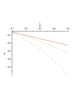
Figure 1: We show the variation of $\beta$ with respect to $\frac{r}{\delta}$ for different values of displacement vector $\beta_{0}$ and choosing other parameters as constants ($\beta_{0}=.1$, for red line; $\beta_{0}=.5$, for green line; $\beta_{0}=1$, for yellow line ).

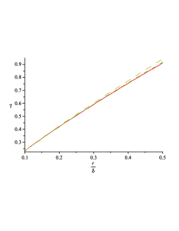
Figure 2: We show the variation of $\gamma$ with respect to $\frac{r}{\delta}$ for different values of displacement vector $\beta_{0}$ and choosing other parameters as constants ($\beta_{0}=.1$, for red line; $\beta_{0}=.5$, for green line; $\beta_{0}=1$, for yellow line ).

Thus the solution for vacuumless cosmic string in Lyra geometry will be taken the following form as

$ds^{2}=\left[1-\frac{3}{2}{\beta_{0}^{2}r^{2}}-\frac{D(n-4)}{(1-b)(2-b)(n+2)}r^{-b+2}\right](-dt^{2}+dz^{2}+dr^{2})+r^{2}\left[1+\frac{1}{8}{\beta_{0}^{2}r^{2}}+\frac{D(3n+4)}{(3-b)(2-b)(n+2)}r^{-b+2}\right]d\theta^{2}$

(20)

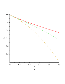
Figure 3: We show the variation of $A\equiv g_{tt}\equiv g_{zz}\equiv g_{rr}$ with respect to $\frac{r}{\delta}$ for different values of displacement vector $\beta_{0}$ and choosing other parameters as constants ($\beta_{0}=.1$, for red line; $\beta_{0}=.5$, for green line; $\beta_{0}=1$, for yellow line ).

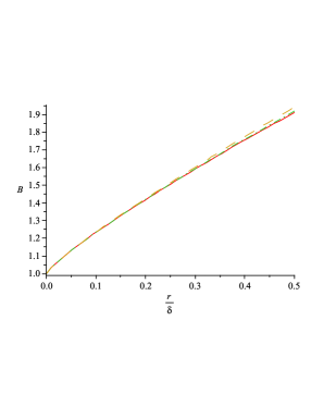
Figure 4: We show the variation of $B\equiv g_{\theta\theta}$ with respect to $\frac{r}{\delta}$ for different values of displacement vector $\beta_{0}$ and choosing other parameters as constants ($\beta_{0}=.1$, for red line; $\beta_{0}=.5$, for green line; $\beta_{0}=1$, for yellow line ).

4. Gravitational effects on test particles :

The repulsive and attractive character of the global string can be discussed by either studying the time like geodesics in the space time or analyzing the acceleration of an observer who is at rest relative to the string.
We now calculate the radial acceleration vector $A^{r}$ of a particle that remains stationary ( i.e. $V^{1}=V^{2}=V^{3}=0$ ) in the field of the string .
Let us consider an observer with four velocity $V_{i}=\sqrt{g_{00}}\delta_{i}^{t}$ .
Now $A^{r}=V^{1}_{;0}V^{0}=\Gamma^{1}_{00}V^{0}V^{0}$.

So for our space time (20),

$$A^{r}=-3{\beta_{0}^{2}r}+\frac{D(-n+4)}{(1-b)(n+2)(1+\beta)^{3}}r^{-b+1}$$ (21)

We see that for $n=2.718608172$ the expression $A^{r}$ is negative and in this case gravitational forces varies with the radial distance. This indicates that particle accelerates towards the string in the radial direction in order to keep it rest. This implies that the string has a repulsive influence on the test particle [24].

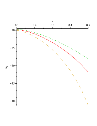
Figure 5: We show the variation of acceleration $(A^{r})$ with respect to r for different values of displacement vector $\beta_{0}$ and choosing other parameters as constants ($\beta_{0}=.3$, for red line; $\beta_{0}=.1$, for green line; $\beta_{0}=.5$, for yellow line ).

5. The Basic Equations for constructing vacuum less global monopole:

According to Bariolla and Vilenkin [25], the monopole is associated with a triplet of scalar fields $\Phi^{a},a=1,2,3.$ and the monopole ansatz is taken as $\Phi^{a}=f(r)\frac{x^{a}}{r}$, where r is the distance from the monopole center. Cho and Vilenkin have shown that for the power law potential (2), the field equation for $f(r)$ admits a solution of the form[2,3]

$$f(r)=aM(\frac{r}{\delta})^{\frac{2}{n+2}}$$ (22)

where $\delta=\frac{1}{M\surd\lambda}$ is the core radius of the monopole , r is the distance from the monopole center and $a=(n+2)^{\frac{2}{n+2}}(n+4)^{-\frac{1}{n+2}}$.

It is argued that the solution (22) can be applied in the region for

$$\delta\ll r\ll R$$ (23)

where the cut off radius R is set by the distance to the nearest anti monopole .

For a vacuum less monopole the space time is static , spherically symmetric and the corresponding line element can be taken as

$$ds^{2}=e^{\nu(r)}dt^{2}-e^{\lambda(r)}dr^{2}-r^{2}(d\theta^{2}+sin^{2}\theta d\phi^{2})$$ (24)

The components of the stress energy tensors for the vacuumless monopole are given by

$$T_{t}^{t}=\frac{(f^{\prime})^{2}}{2e^{\lambda(r)}}+\frac{f^{2}w^{2}}{r^{2}}+\frac{1}{2e^{2}r^{2}}\left[\frac{(w^{\prime})^{2}}{e^{\lambda(r)}}+\frac{(1-w^{2})^{2}}{2r^{2}}\right]+V(f)$$ (25)

$$T_{r}^{r}=-\frac{(f^{\prime})^{2}}{2e^{\lambda(r)}}+\frac{f^{2}w^{2}}{r^{2}}+\frac{1}{2e^{2}r^{2}}\left[\frac{(w^{\prime})^{2}}{e^{\lambda(r)}}+\frac{(1-w^{2})^{2}}{2r^{2}}\right]+V(f)$$ (26)

$$T_{\theta}^{\theta}=T_{\phi}^{\phi}=\frac{(f^{\prime})^{2}}{2e^{\lambda(r)}}+\frac{1}{2e^{2}r^{2}}\left[\frac{(w^{\prime})^{2}}{e^{\lambda(r)}}+\frac{(1-w^{2})^{2}}{2r^{2}}\right]+V(f)$$ (27)

For monopole, the gauge field is $A_{i}^{a}(r)=\frac{[1-w(r)]\epsilon^{aij}x^{j}}{er^{2}}$ . $T_{a}^{b}$ ’s with $w=1$ are that for global monopole. For global vacuum less monopole, one can use the flat space approximation for $f(r)$ in (22) as well as $V(f)$ given in in (2) for $r\gg\delta$.
This follows from the fact that in this case the gravity would not much influence on monopole structure.

Here the field equations are

$$e^{-\lambda}\left[-\frac{\lambda^{\prime}}{r}+\frac{1}{r^{2}}\right]-\frac{1}{r^{2}}+\frac{3}{4}e^{-\nu}\beta_{0}^{2}=8\pi GCr^{-b}$$ (28)

$$e^{-\lambda}\left[\frac{1}{r^{2}}+\frac{\nu^{\prime}}{r}\right]-\frac{1}{r^{2}}-\frac{3}{4}e^{-\nu}\beta_{0}^{2}=8\pi GDr^{-b}$$ (29)

$$\frac{1}{2}e^{-\lambda}\left[\frac{1}{2}(\nu^{\prime})^{2}+\nu^{\prime\prime}-\frac{1}{2}\lambda^{\prime}\nu^{\prime}+\frac{1}{r}({\nu^{\prime}-\lambda^{\prime}})\right]+\frac{3}{4}e^{-\nu}\beta_{0}^{2}=8\pi GEr^{-b}$$ (30)

where

$C=\left[\frac{2a^{2}M^{2}}{2(n+2)}+a^{2}M^{2}+\frac{M^{2}}{a^{2}}\right]\delta^{\frac{-4}{n+2}},\\ D=\left[-\frac{2a^{2}M^{2}}{2(n+2)}+a^{2}M^{2}+\frac{M^{2}}{a^{2}}\right]\delta^{\frac{-4}{n+2}},\\ E=\left[\frac{2a^{2}M^{2}}{2(n+2)}+\frac{M^{2}}{a^{2}}\right]\delta^{\frac{-4}{n+2}},\\ b=\frac{2n}{(n+2)}.$

6. Solutions in the weak field approximations :

Now we will consider the solution of a vacuumless monopole in the weak field approximation. At this stage, let us assume that

$e^{\nu(r)}=1+f(r),e^{\lambda(r)}=1+g(r).$

where $f,g\ll 1$.
In this approximations $eqs.(9)-(12)$ take the following forms as

$$\frac{g}{r^{2}}+\frac{g^{\prime}}{r}-\frac{3}{4}\beta_{0}^{2}=-8\pi GCr^{-b}$$ (31)

$$-\frac{g}{r^{2}}+\frac{f^{\prime}}{r}-\frac{3}{4}\beta_{0}^{2}=8\pi GDr^{-b}$$ (32)

$$f^{\prime\prime}+\frac{(f^{\prime}-g^{\prime})}{r}-\frac{3}{4}\beta_{0}^{2}=8\pi GEr^{-b}$$ (33)

Solving these equations , we get

$$g=\frac{1}{4}r^{2}\beta_{0}^{2}-\left[\frac{8\pi GC}{(3-b)}\right]r^{2-b}$$ (34)

$$f=\frac{1}{2}r^{2}\beta_{0}^{2}-\left[\frac{8\pi G}{(2-b)}\right]\left[\frac{-D+C}{(3-b)}\right]r^{2-b}$$ (35)

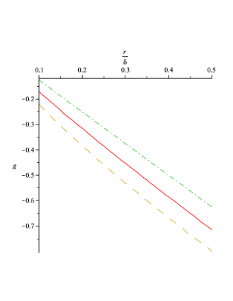
Figure 6: We show the variation of $g$ with respect to $\frac{r}{\delta}$ for different values of n and choosing other parameters as constants ($n=2.5$, for red line; $n=2$, for green line; $n=3$, for yellow line ).

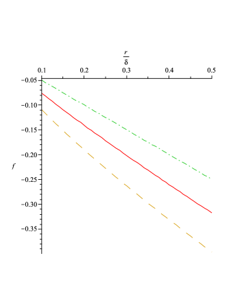
Figure 7: We show the variation of $f$ with respect to $\frac{r}{\delta}$ for different values of n and choosing other parameters as constants ($n=2.5$, for red line; $n=2$, for green line; $n=3$, for yellow line ).

Thus the solution for vacuumless global monopole in Lyra geometry will be taken the following form as

$$ds^{2}=\left[1+\frac{1}{2}r^{2}\beta_{0}^{2}+\pi GM^{2}K(n)\left(\frac{r}{\delta}\right)^{2-b}\right]dt^{2}-\left[1+\frac{1}{4}r^{2}\beta_{0}^{2}+\pi GM^{2}C(n)\left(\frac{r}{\delta}\right)^{2-b}\right]dr^{2}-r^{2}d\Omega_{2}^{2}$$ (36)

where $K(n)$ and $C(n)$ are complicated functions of n. If we put $\beta_{0}=0$ i.e. in the absence of the displacement vector our metric transforms to

$$ds^{2}=\left[1+\pi GM^{2}K(n)\left(\frac{r}{\delta}\right)^{2-b}\right]dt^{2}-\left[1+\pi GM^{2}C(n)\left(\frac{r}{\delta}\right)^{2-b}\right]dr^{2}-r^{2}d\Omega_{2}^{2}$$ (37)

which is same form of $CV^{{}^{\prime}s}$ solution in general relativity.

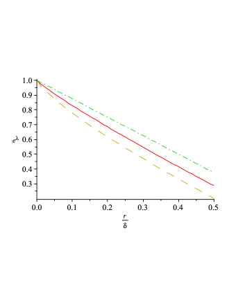
Figure 8: We show the variation of $e^{\lambda}$ with respect to $\frac{r}{\delta}$ for different values of n and choosing other parameters as constants ($n=2.5$, for red line; $n=2$, for green line; $n=3$, for yellow line ).

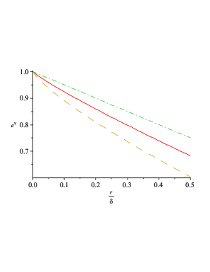
Figure 9: We show the variation of $e^{\nu}$ with respect to $\frac{r}{\delta}$ for different values of n and choosing other parameters as constants ($n=2.5$, for red line; $n=2$, for green line; $n=3$, for yellow line ).

7. Gravitational effects on test particles :

Let us consider a relativistic particle of mass m,moving in the gravitational field of monopole described by equation (36) .
According to the formalism of Hamilton and Jacobi (H-J), the H-J equation is [26]

$$\frac{1}{B(r)}(\frac{\partial S}{\partial t})^{2}-\frac{1}{A(r)}(\frac{\partial S}{\partial r})^{2}-\frac{1}{r^{2}}(\frac{\partial S}{\partial\theta})^{2}-\frac{1}{r^{2}\sin^{2}\theta}(\frac{\partial S}{\partial\phi})^{2}+m^{2}=0$$ (38)

where

$B(r)=\left[1+\frac{1}{2}r^{2}\beta_{0}^{2}+\pi GM^{2}K(n)\left(\frac{r}{\delta}\right)^{2-b}\right]$ and $A(r)=\left[1+\frac{1}{4}r^{2}\beta_{0}^{2}+\pi GM^{2}C(n)\left(\frac{r}{\delta}\right)^{2-b}\right]$

In order to solve the particle differential equation , let us use the separation of variables for the H-J function S as follows [26] .

$$S(t,r,\theta,\phi)=-Et+S_{1}(r)+S_{2}(\theta)+J\phi$$ (39)

Here the constants E and J are identified as the energy and angular momentum of the particle .
The radial velocity of the particle is( For detail calculations see reference (26) ).

$$\frac{dr}{dt}=\frac{B}{E\sqrt{A}}\sqrt{\frac{E^{2}}{B}+m^{2}-\frac{p^{2}}{r^{2}}}$$ (40)

where $p$ is the separation constant .

The turning points of the trajectory are given by $\frac{dr}{dt}=0$ and as a consequence the potential curves are

$$\frac{E}{m}=\sqrt{\left[1+\frac{1}{2}r^{2}\beta_{0}^{2}+\pi GM^{2}K(n)\left(\frac{r}{\delta}\right)^{2-b}\right]\left[\frac{p^{2}}{m^{2}r^{2}}-1\right]}\equiv V$$ (41)

In this case the extremals of the potential curve are the solutions of the equation

$$m^{2}H(2-b)r^{4-b}+bHr^{2-b}+m^{2}r^{4}\beta_{0}^{2}-2p^{2}=0$$ (42)

where $H=\pi GM^{2}K(n)\delta^{b-2}$.

This equation has at least one positive real root provided (-b+2) is an positive integer. So it is possible to have bound orbit for the test particle. Thus the gravitational field of the vacuumless global monopole is shown to be attractive in nature but here we have to imposed some restriction on the constant ”n”. This effect is absent in general relativity case.

8. Conclusion :

Observations of the flatness of galactic rotation curves indicate the galaxies, cluster of galaxies and super clusters are filled out with 90 percent of nonluminous matter (dark matter). Recently, it has been suggested that some of the topological defects such as monopole could be present in the galactic dark matter and these topological defects are responsible for the structure formation of the Universe [27-30]. So, topological defects have been revived in the recent years. This work extends the earlier work by Cho and Vilenkin regarding the gravitational field of a vacuumless topological defects, namely, cosmic string and global monopole to the scalar tensor theory based on Lyra geometry. We see that in going from general relativity to scalar tensor theory based on Lyra geometry both space time curvature and topology are affected by the present of the displacement vector. Our study of the motion of the test particle reveals that the vacuumless global string in Lyra geometry exerts gravitational force which is repulsive in nature. It is similar to the case of a vacuumless global string in general relativity where the vacuumless global string in general relativity has repulsive gravitational effect.
Whereas vacuumless global monopole in Lyra geometry exerts gravitational force which is attractive in nature. It is dissimilar to the case of a vacuumless global monopole in general relativity. In the absence of the displacement vector i.e. $\beta_{0}=0$, our solution coincides with CV solution (with proper choices of the arbitrary constants). Since our vacuumless monopole exerts gravitational pull on surrounding particles, so it seems important to consider vacuumless monopole field as a candidate for galactic dark matter.

References

[1]
[2] Kibble,T.W.B.J.Phys.A 9,1387(1976);
A.Vilenkin and E.P.S.Shellard(1994), Cosmic String and
other Topological Defects (Camb.Univ.Press)
[3] I.Cho and A.Vilenkin Phys.Rev.D 59,021701 (1999)
[4] I.Cho and A.Vilenkin Phys.Rev.D 59,063510 (1999)
[5] I. Zlatev et al, Phys.Rev.Lett. 80, 1582 (1999)
[6] Lyra. G , Math. Z 54,52 (1951)
[7] Brans C and Dicke R.H, Phys.Rev. 124,
925(1961)
[8] Sen D. K and Dunn K. A , J. Math. Phys 12, 578 (1971)
[9] A Beesham , Ast. Sp. Sc 127, 189 (1986)
[10] T. Singh and G.P. Singh , J. Math. Phys. 32, 2456(1991)
[11] Rahaman F and Bera J , Int.J.Mod.Phys.D 10,729(2001)
[12] Anirudh Pradhan, I. Aotemshi , Astrophys.Space Sci.288:315 (2003)
[13]D.R.K.Reddy and M.V.SubbaRao ,Astrophys.Space Sci.302,157(2006)
[14] Jerzy Matyjasek , Int.J.Theor.Phys.33, 967 (1994)