Flexible Multivariate Density Estimation with Marginal Adaptation

Abstract

Our article addresses the problem of flexibly estimating a multivariate density while also attempting to estimate its marginals correctly. We do so by proposing two new estimators that try to capture the best features of mixture of normals and copula estimators while avoiding some of their weaknesses. The first estimator we propose is a mixture of normals copula model that is a flexible alternative to parametric copula models such as the normal and $t$ copula. The second is a marginally adapted mixture of normals estimator that improves on the standard mixture of normals by using information contained in univariate estimates of the marginal densities. We show empirically that copula based approaches can behave much better or much worse than estimators based on mixture of normals depending on the properties of the data. We provide fast and reliable implementations of the estimators and illustrate the methodology on simulated and real data.

Keywords: Copula, mixture of normals, nonparametric, stochastic approximation.

1 Introduction

Our article is concerned with flexible and practical estimation of multivariate densities, that is, with constructing estimators that are computationally reliable and statistically efficient when the data generating process is unknown. Since a multivariate density is determined by the densities of all linear combinations of its marginal variables (that is, by its characteristic function), this suggests that an effective multivariate density estimator is one that can estimate reliably the densities of all such linear combinations, and in particular the marginal densities.

A common approach to multivariate density estimation is to use a parametric density such as a normal or a $t$. Such densities are relatively easy to estimate and there is extensive finite sample inference available for them; e.g. Anderson (2003). Estimation methods and inference for more general parametric densities such as symmetric and skew symmetric elliptic densities are also available; e.g. Genton (2004). An important advantage of parametric densities is that they can be applied to high dimensional problems because of the relatively small number of parameters involved. However, the small number of parameters can also be a major disadvantage if the data generating process differs significantly from the parametric model. For example, if bivariate data is modeled as a bivariate normal distribution then just one parameter (the correlation coefficient) is available to capture the dependence between the two marginals.

Parametric or semiparametric copula models such as the multivariate normal or $t$ (Joe, 1997; Nelsen, 1999) provide extra flexibility in density estimation by separately modeling the marginal densities and then linking them through a joint parametric model of dependence such as the multivariate normal or $t$ distribution (Joe, 1997; Nelsen, 1999). For example, a Gaussian copula approach to density estimation models each marginal separately using a parametric (or possibly nonparametric) model and then transforms each marginal to a standard normal. These transformed marginals are then modeled as a multivariate normal distribution. See also Demarta and McNeil (2005) for two parametric generalizations of the $t$ copula, the skewed $t$ and the grouped $t$ copulas. We note that an attractive feature of copula models is that the marginal densities implied by the copula density are the same as those originally proposed for the marginals. In addition, by transforming each marginal to a standard distribution such as a standard normal there is some hope that the joint distribution of the transformed variables will also behave ‘nicely’.

In general, however, the use of parametric copula models to capture dependence is likely to have the same advantages and disadvantages as conventional parametric models. Thus, suppose that we have bivariate observations with each marginal having support on $m$ points so that the joint distribution has support on $m^{2}$ points. If we model the bivariate distribution using a Gaussian copula then we may hope to capture the distribution of each marginal that has support on $m$ points through an appropriate model for that marginal. However, the Gaussian copula only allows one extra parameter (the correlation coefficient) to capture the joint dependence contained in the remaining $m^{2}-2m$ points of support. Clearly, such modeling problems increase as $m$ increases and as the dimension $p$ of the multivariate vector increases.

To overcome the problems encountered using parametric methods, there is a large and growing literature on nonparametric density estimation. One popular approach is kernel density estimation. Sheather (2004) surveys the univariate case and makes it clear that the critical aspect of the method is the choice of smoothing or bandwidth parameter. We infer from Sheather’s article that it will be challenging to successfully apply kernel density estimation in higher dimensions. A second approach is to use finite mixture of normals; see for example McLachlan and Peel (2000) for a discussion of univariate and multivariate approaches to estimation, and Richardson and Green (1997) and Roeder and Wasserman (1997) for fully Bayesian univariate analyses. A third approach is to use Dirichlet Process Mixtures (DPM) which in many applications is equivalent to an infinite mixture of normals with constraints on the mixing probabilities; see Green and Richardson (2001) for a comparison of finite mixture models and DPM. We note, however, that one of the problems encountered by estimating densities by mixture models, especially in higher dimensions, is that in finite samples the implied model for each marginal may not be even close to the best model for that marginal. To understand why, consider the example of a multivariate distribution with $p$ independent marginals (possibly all identical) where each marginal is a mixture of $m$ normals. Then the joint distribution is also a mixture of normals, but with $m^{p}$ components so that for moderate values of $m$ and $p$ it will usually be unrealistic to fit a multivariate mixture model with so many components as such a model will be highly over-parametrized. See Section 3.3.1 for further discussion.

We propose two new estimators of multivariate densities that attempt to capture the advantages of parametric copula estimators and mixture of normals estimators while being more robust to their weaknesses. The first estimator is a mixture of normals copula (MNC) where we flexibly estimate each of the marginals, transform the marginals to standard normal distributions, and then flexibly estimate the joint distribution through a mixture of normals with approximately normal marginals. This defines a more flexible copula than currently available in the literature.

We show through simulation that the mixture of normals copula performs well when the data are generated by a normal or $t$ copula, but that a normal and $t$ copula can provide a poor fit when the assumed model is incorrect. A mixture of normals and a mixture of normals copula are both universal approximations to any multivariate density when the number of components is estimated from the data. That is, given enough data they will provide accurate approximations to any multivariate density. However, and contrary to our initial intuition, either can greatly outperform the other in any given dataset. In moderate to large dimensions, copulas tend to perform poorly when the joint distribution is non-normal but well modeled by a mixture of normals with few components. Conversely, a mixture of normals can be grossly inadequate when a normal or $t$ copula fits the data well. An example of this occurs when $p$ variables have non-normal distributions but weak dependence.

Motivated by these findings we introduce a second density estimator, the marginally adapted mixture of normals, where we correct the mixture of normals density estimator by a factor that reflects the difference between the univariate and multivariate estimates of the marginal distribution of each variable. If the marginals are well approximated by univariate estimators, then this estimator can be shown to be at least as good as a mixture of normals in a sense made precise in Section 4. In practice, the marginally adapted mixture of normals can be expected to improve on the standard mixture of normals whenever the density cannot be well approximated using only a small number of components. We also note that marginal adaptation of multivariate densities is a general concept that can be applied outside the mixture of normals framework.

The mixture of normals model is the basic building block of our estimators. This is not a simple model to fit because the likelihood can be multimodal and badly behaved. See for example McLachlan and Peel (2000, Chapter 3). We implement our methods using the computationally efficient and fast stochastic approximation algorithms described in Appendix B.

2 Estimating the normal, $t$ and mixture of normals copulas

We briefly introduce copulas and refer to Joe (1997) and Nelsen (1999) for a modern treatment. The multivariate function ${C}(\bm{u})={C}(u_{1},...,u_{p})$ is a copula if it is a multivariate cumulative distribution function (cdf) on the $p$-dimensional cube $[0,1]^{p}$ with uniformly distributed marginals. If $U_{1},\dots,U_{p}$ are the corresponding $p$ marginal variables then

$${C}(\bm{u})=\Pr(U_{1}\leq u_{1},...,U_{p}\leq u_{p}).$$ (1)

We can construct a copula model explicitly for a random vector $\bm{y}=(y_{1},\dots,y_{p})$ by choosing a copula ${C}(\bm{u})$ with $\bm{u}$ obtained by transforming each $y_{j}$ to a uniform using its marginal cdf so that $u_{j}=H_{j}(y_{j})$. However, the more popular copulas are defined implicitly on transformations of $\bm{u}$ as follows. Suppose that $\bm{x}$ is a multivariate $p$ dimensional random variable with density $f(\bm{x})$ and cdf $F(\bm{x})$, and corresponding marginal densities and cdf’s $f_{j}(x_{j})$ and $F_{j}(x_{j}),j=1,\dots,p$. We now define one to one transformations of $\bm{x}$ to $\bm{y}$ by $F_{j}(x_{j})=u_{j}=H_{j}(y_{j})\ ,j=1,\dots,p$ . Then the implied density of $\bm{y}$ is

$$p(\bm{y})=f(\bm{x})\prod\limits_{j=1}^{p}\biggl{(}h_{j}(y_{j})/f_{j}(x_{j})\biggr{)}.$$ (2)

For example, a normal or Gaussian copula is defined implicitly by taking $x$ as multivariate normal with zero mean and with standard normal marginals.

Joint estimation of both the copula and marginal parameters is challenging even in problems of moderate dimension. The standard approach fits separate models to each marginal and treats the resulting distributions as fixed when estimating the copula. We also follow this two-stage approach. Joe (1997) and in the Bayesian literature Pitt et al. (2006) fit parametric distributions to the marginals. A more common procedure estimates the marginals nonparametrically using the marginal empirical distribution functions, as in Demarta and McNeil (2005). We model the marginals as a mixture of normals. This is more computationally demanding than the nonparametric approach based on the marginal empirical distributions, but should give a more efficient estimate of the joint distribution function in small samples and is better suited to incorporating regression effects.

Appendices A.1 and A.2 outline how we estimate the normal and $t$ copulas.

2.1 Mixture of normals copula

We propose to define and estimate a mixture of normals copula as follows. Steps one and two are the same as for a normal copula. In step three, we fit a mixture of normals to $x,$ with the number of components chosen by BIC. The parameters of the mixture of normals implicitly define the copula.

The one component case is a normal copula, estimated exactly as in appendix A.1. With more than one component, the parameters estimated in step three will not imply exactly standard normal marginals. This discrepancy between steps two and three implies a small efficiency loss in small samples, but poses no theoretical problem, since any multivariate distribution for $\bm{x}$ implicitly defines a copula as long as the density $p(\bm{y})$ is computed as in equation (2). When evaluating or drawing from $p(\bm{y})$ one must therefore take into account that the marginal distribution $f_{j}(x_{j})$ in this case is not standard normal but a mixture of normals. Moreover, the one-to-one transformation $x_{j}=F_{j}^{-1}(H_{j}(y_{j}))$ which implicitly defines the copula requires that for use in (2) we recompute $\bm{x}$ using the mixture of normals parameters to define $F_{j}$.

3 A comparison of estimators

This section investigates empirically the performance of various copula based estimators, a mixture of normals estimator and a skew $t$ estimator for different data generating process (DGP). The main conclusions are that (i) we can expect the mixture of normals copula to rarely perform much worse than a $t$ copula in problems of moderate dimensions, while the contrary need not hold; (ii) both $t$ and mixture of normals copulas can fit either much better or much worse than mixture of normals depending on the data generating process.

Simulation design.

In all the simulation experiments we use a sample of $n=500$, $p=5$ variables and 50 replications. All the copula data generating processes share the same marginals, which are a mixture of normals. The number of components for all mixture of normals, whether in copulas or stand-alone, is chosen by BIC in the range $1$ to $10$ (where $10$ was never chosen in our simulations). The estimation process and the tuning parameters for the mixture of normals estimators are described in Appendix B.

We use the Kullback-Liebler divergence and the $L_{2}$ distance of the estimate from the true model to compare the performance of the various estimators. The results are reported relative to a given estimator, usually the estimator corresponding to the data generating process. The Kullback-Liebler divergence between the estimate $\widehat{p}(\bm{y})$ and the true density $p(\bm{y})$ is

$$KL(p,\widehat{p}) =\int p(\bm{y})\log\biggl{(}\frac{p(\bm{y})}{\widehat{p}(\bm{y})}\biggr{)}d\bm{y}\ .$$ (3)

We estimate (3) by

$$\widehat{KL}(p,\widehat{p}) =N^{-1}\sum_{i=1}^{N}\log\biggl{(}\frac{p(\bm{y}_{i})}{\widehat{p}(\bm{y}_{i})}\biggr{)}\ ,$$ (4)

where $\bm{y}_{i},i=1,\dots,N$ are a sample of $N=5000$ observations drawn from the $p(\bm{y})$ and which are different from the observations used to estimate each model. The $L_{2}$ loss is defined as

$$L_{2}(p,\widehat{p}) =\int\biggl{(}p(\bm{y})-\widehat{p}(\bm{y})\biggr{)}^{2}d\bm{y}$$

and is estimated by

$${\widehat{L}}_{2}(p,\widehat{p}) =N^{-1}\sum_{i=1}^{N}\biggl{(}p(\bm{y}_{i})-\widehat{p}(\bm{y}_{i})\biggr{)}^{2}/p(\bm{y}_{i})\ ,$$

where the $\bm{y}_{i}$ are defined similarly to (4).

Our simulations considered a number of data generating processes which are discussed below and the following estimators. (a) The normal copula (NC). (b) The $t$ copula with estimated degrees of freedom (tC). (c) The mixture of normals copula (MNC). (d) The Clayton, Frank and Gumbel Archimedian copulas described briefly in Appendix C. (e) The mixture of normals estimator (MN). (d) The multivariate skew $t$ estimator (ST) in Sahu et al. (2003), whose aim is to capture both multivariate skewness and kurtosis. This estimator is described briefly Appendix D. For all copulas, the marginals were estimated by a mixture of normals.

A more comprehensive set of simulations is reported in Giordani et al. (2008), which is an extended version of the current article.

3.1 Normal copula data generating process

The data generating process for this simulation has marginals that are mixtures of normals with three components, with means $\mu_{j,1}=0,$ $\mu_{j,2}=-3,$ $\mu_{j,3}=3$, component probabilities $\pi_{j,1}=0.6$ and $\pi_{j,2}=0.2,$ and component variances $\sigma_{j,1}^{2}=1,$ $\sigma_{j,2}^{2}=9,$ $\sigma_{j,3}^{2}=0.1,$ for $j=1,...,p,$. The copula is $N(0,\bm{V})$ with $\bm{V}=0.5\bm{I}+0.5\bm{i}\bm{i}^{T},$ and $\bm{i}$ the unit vector. Table 1 reports the median of the logarithm of the ratio of KL divergence for a particular estimator and the KL divergence of the $t$ copula estimator over the 50 replicates. If we multiply each entry in the table by 100 then we can interpret each entry as approximately the median percentage increase in KL divergence of the particular estimator relative to the $t$ copula estimator. The table also shows those log ratios that are not significantly different from 0 at the 1% and 5% levels as judged by the Wilcoxon rank sum test. The entries for the $L_{2}$ loss function are interpreted similarly. We work with the logarithm of the ratios of the loss functions as these are distributed closer to normality than the ratios them selves. When two estimators perform similarly relative to a loss function, we would expect the median of the logarithm of the ratios to be approximately zero and this is why we report this median.

Since the number of components in the mixture of normals copula is chosen by BIC rather than fixed, we expect it to perform nearly as well as a normal copula even when the latter generates the data. This is confirmed by the simulation results reported in Table 1. The normal, $t$ and mixture of normals copulas perform similarly. In particular, the BIC criterion almost always selects one component for the mixture of normals copula so the loss of efficiency from estimating a mixture of normals copula copula is negligible. However, the losses for the three Archimedian copula are substantial despite the marginals being estimated flexibly. The losses for the mixture of normals estimator and the skew t estimator can also be substantial.

3.2 Archimedian copula data generating processes

Table 2 presents simulation results when the data generating process is a Clayton copula with parameter $\theta=5$ and with the same marginals as in Section 3.1. The table shows that the mixture of normals copula performs best overall, and that the two other Archimedian copulas do not perform very well when the true data generating process is a Clayton copula.

3.3 Comparing a mixture of normals copula to a mixture of normals

One may expect a mixture of normals copula and a mixture of normals to perform similarly in any given dataset. In fact, either can greatly outperform the other depending on the characteristics of the density to be approximated. It is useful to consider two reasons why a mixture of normals copula may fit better (worse) than a mixture of normals: (i) direct estimation of the marginals is more (less) accurate than indirect estimation through the joint distribution; (ii) the transformed variables $x,$ with normal marginals, are easier (more difficult) to fit with a mixture of normals than the original variables $y$. We now discuss this issue conceptually and report some simulation results.

3.3.1 Direct vs indirect estimation of the marginal densities.

Indirect estimation of the marginal densities through the joint distribution is more efficient if the model for the joint is correct, but less robust to model misspecification. Consider a deceptively mild form of model misspecification, namely over-parameterization. Assume that the data generating process is a mixture of normals. Define the degree of over-parametrization as the number of valid exact restrictions not imposed on the parameters of a mixture of normals over the total number of estimated parameters. A mixture of normals copula can be expected to outperform a mixture of normals when the degree of over-parameterization is high.

For example, suppose that $p$ independent variables are each generated by the same univariate mixture with $m$ components. That is, the marginal densities are all identical. However, the joint distribution is a mixture of normals with $m^{p}$ components. In this case, a mixture of normals quickly becomes highly over parametrized as $p$ gets larger, while a mixture of normals copula will fit the marginals parsimoniously and then use one component for the copula. For medium and large $p$, a mixture of normals copula should therefore outperform a mixture of normals in this example. The simulations reported in Table 1 and other simulations not reported in the article confirm this analysis. The ability of a mixture of normals to fit the data generating process deteriorates very quickly with $p.$ The results are even worse if we set $\bm{V}=\bm{I}$ rather than $\bm{V}=0.5\bm{I}+0.5\bm{ii}^{T}$ (not reported).

Less extreme cases are likely to occur in empirical applications. For example, if the variables can be divided into $l$ groups, each a mixture of $m$ components independent of the other group, a mixture of normals for the joint distribution requires $m^{l}$ components. In these situations the over-parametrization will typically result in poor fit and in the model selection criteria choosing less components than in the data generating process (a mixture of factor analyzers should perform better in these cases).

3.3.2 Fitting $\bm{x}$ vs fitting $\bm{y}$.

In the simulations summarized in Table 1, $\bm{x}$ is multivariate normal and $t$ respectively, making it easier to model than $\bm{y}$. However, when the data cluster, $\bm{x}$ can be much more difficult to fit than $\bm{y}$. The cluster representation evident in $\bm{y}$ can be severely distorted in the $\bm{x}$, making the multivariate distribution of $\bm{x}$ extremely complex. Consider data generated by a mixture of three well-separated bivariate normals

$$p(\bm{y})=\frac{1}{3}\phi_{2}(\bm{y};\bm{0},\bm{I})+\frac{1}{3}\phi_{2}(\bm{y};-5\bm{i},\bm{I})+\frac{1}{3}\phi_{2}(\bm{y};5\bm{i},\bm{I}),$$

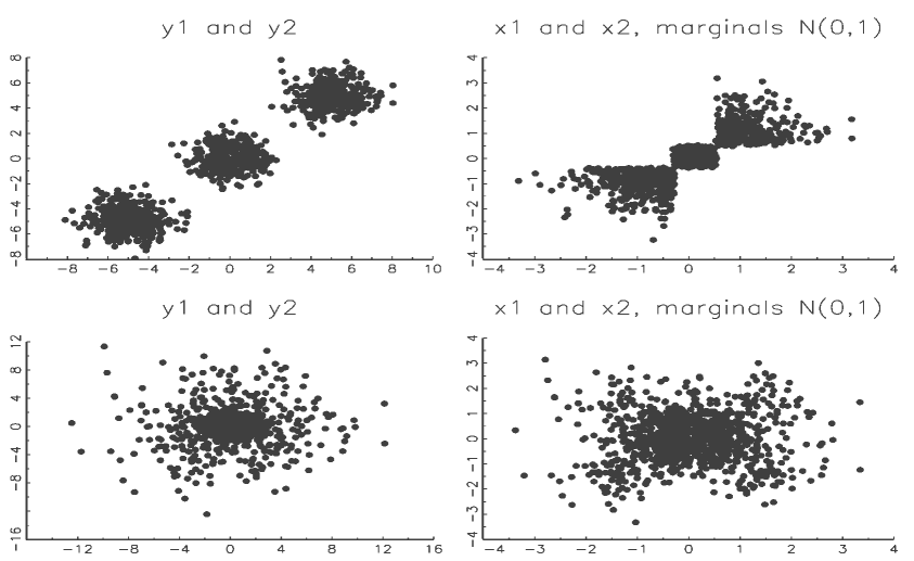
Figure 1: First row. 1000 observations generated by a bivariate mixture of 3 normals $(y_{1},y_{2})$ and corresponding $x_{1},x_{2}$ with $N(0,1)$ marginals obtained through the true marginal densities of $y_{1}$ and $y_{2}$. Second row. As for the first row, observations generated by a scale mixture of two normals. See Section 3.3.2.

where $\bm{i}$ is defined above and $\phi_{p}(\bm{\mu},\bm{\Sigma})$ is a $p$-dimensional multivariate normal density with mean $\bm{\mu}$ and variance $\bm{\Sigma}$. The first row of Figure 1 shows 1000 observations generated from this data generating process together with the $\bm{x}$ obtained through the true marginal densities. It is clear that the fact that $\bm{x}$ has standard normal marginals is of little comfort, as the joint distribution of $\bm{x}$ is extremely difficult to model. Overlapping clusters also cause trouble for copulas, though not as dramatically. Consider data generated by a scale mixture of two normals

$$p(\bm{y})=0.6\phi_{2}(\bm{y};\bm{0},\bm{I})+0.4\phi_{2}(\bm{y};\bm{0},16\bm{I}),$$

from which we generate 1000 observations, as displayed in the second row of Figure 1. Clearly more than two components are needed to capture the joint density of $\bm{x}$ adequately.

The simulation results reported in Table 3 confirm this analysis. To emphasise the point that the clusters need not be separated for copulas to work poorly, the data are generated by a scale mixture of two normals

$$p(\bm{y})=0.7\phi_{p}(\bm{y};\bm{0},\bm{I})+0.3\phi_{p}(\bm{y};\bm{0},4\bm{I}+5\bm{ii}^{T}).$$

The normal copula performs very poorly. The $t$ copula is better but still poor. The mixture of normals copula improves on the $t$ copula but still produces large losses compared to a mixture of normals.

4 Marginally adapted multivariate densities

The discussion in the previous section highlights an important trade-off involved in estimating multivariate distributions. To capture the dependence structure of a set of variables parsimoniously we usually need to place strong constraints on their marginal densities and, conversely, focusing on the marginal densities may make it harder to model the dependence effectively. Motivated by these results we introduce the class of marginally adapted densities. The idea is to fit a multivariate density to the original data and then correct it by a factor reflecting the discrepancy between the marginal distributions implied by the multivariate model and those fitted directly to each variables. If the second set of marginals is more accurate than the first, the marginally adapted density is likely to be closer to the true density in a sense that is made precise below.

Suppose that $f(\bm{y})$ and $h(\bm{y})$ are $p$ dimensional densities with respect to Lebesgue measure with marginal densities $f_{i}(y_{i}),h_{i}(y_{i})$ , $i=1,\ldots,p$. For $0\leq\varepsilon\leq 1$, let $f_{i,\varepsilon}(y_{i})=(1-\varepsilon)f_{i}(y_{i})+\varepsilon h_{i}(y_{i})$, for $i=1,\dots,p$. Then each $f_{i,\varepsilon}(y_{i})$ is a density and $h_{i}(y_{i})/f_{i,\varepsilon}(y_{i})\leq 1/\varepsilon$ for $\varepsilon>0$. Let

$$p_{h,\varepsilon}(\bm{y}) =k_{h,\varepsilon}f(\bm{y})\prod\limits_{i=1}^{p}h_{i}(y_{i})/f_{i,\varepsilon}(y_{i})\ ,$$ (5)

where $k_{h,\varepsilon}$ is a normalizing constant that makes $p_{h,\varepsilon}(y)$ a density for $\varepsilon>0$. We say that $p_{h,\varepsilon}(\bm{y})$ is the density of $f$ adjusted for the marginals $h_{i}$. The following result will give necessary and sufficient conditions for $p_{h,\varepsilon}(\bm{y})$ to be closer to $h$ than $f$ in KL divergence, where the KL divergence is defined by (3).

Lemma 1. Suppose that $f$ and $h$ are $p$ dimensional multivariate densities with the marginals $f_{i}$ and $h_{i}$. Then, for $0<\varepsilon\leq 1$,

$$KL(h,f)-KL(h,p_{h,\varepsilon}) =\log(k_{h,\varepsilon})+\sum\limits_{i=1}^{p}{KL(h_{i},f_{i,\varepsilon})}\ .$$

Proof.

$$KL(h,f)-KL(h,p_{h,\varepsilon}) =\int{h\log\left({p_{h,\varepsilon}(\bm{y})/f(\bm{y})}\right)}d\bm{y}$$

$$=\log(k_{h,\varepsilon})+\sum_{i=1}^{p}\int h(\bm{y})\log\left(h_{i}(y_{i})/f_{i,\varepsilon}(y_{i})\right)d\bm{y}$$

$$=\log(k_{h,\varepsilon})+\sum_{i=1}^{p}\int h(y_{i})\log\left(h_{i}(y_{i})/f_{i,\varepsilon}(y_{i})\right)dy_{i}$$

and the result follows.

The lemma shows that $KL(h,f)>KL(h,p_{h,\varepsilon})$ if

$$\log(k_{h,\varepsilon})+\sum\limits_{i=1}^{p}{KL(h_{i},f_{i,\varepsilon})} >0.$$ (6)

We note that the sum $\sum_{i}{KL(h_{i},f_{i,\varepsilon})}>0$ unless $h_{i}=f_{i,\varepsilon}$ almost everywhere for all $i$ by the properties of the KL divergence. Thus, $KL(h,f)>KL(h,p_{h,\varepsilon})$ is likely to hold if $k_{h,\varepsilon}$ is close to 1. We also note that the condition (6) can be verified for any given $f$ if we know the marginals $h_{i}$, but not necessarily the joint density $h$.

We apply Lemma 1 as follows. Let $h$ be the true multivariate density and $f$ an approximation (or estimate) of it. Suppose that we know the marginals of $h$, but not $h$ itself. Then we can compute $k_{h,\varepsilon}$ and determine whether $KL(h,f)>KL(h,p_{h,\varepsilon})$ using (6). We note the following:

1. Condition (6) can be verified for any given $f$ if we know the marginals $h_{i}$, but not necessarily the joint density $h$.

2. The marginally adaptive density estimator (5) is not in general a copula since its marginals are not necessarily $h_{i}(y_{i}).$

3. We also note that the result of the lemma is very general and does not require either $f(\bm{y})$ or the $h_{i}(y_{i})$ to be a mixture of normals. It can be applied to both simpler more complex models. A simple model could be a multivariate $t$ distribution (or any other parametric multivariate density), with marginals also $t$ distributions (but each with possibly different degrees of freedom) or a mixture of normals or nonparametric kernel density estimates. A more complex model for $f(\bm{y})$ could be a factor model in high dimensional data.

4. Lemma 1 assumes that the marginal distributions $h_{i}(y_{i})$ are known. In practice the marginals $h_{i}(y_{i})$ are estimated from the data and we take $\varepsilon=0.05$.

4.1 Marginally adapted mixture of normals

The marginally adapted mixture of normals (MAMN) estimator specifies $f(\bm{y})$ as a multivariate mixture of normals density, so that its marginals are also mixture of normals and therefore straightforward to compute. The marginally adjusted mixture of normals retains the ability of the mixture of normals to model clustering (overlapping or not) while reducing the risk of poor fitting of the marginal densities. We choose to model $h_{i}(y_{i})$ as a univariate mixture of normals, but we could use any other model estimate.

Estimating $k_{h,\varepsilon}$.

In general there is no analytical expression for the normalizing constant $k_{h,\varepsilon}$ so we estimate it by importance sampling as

$$k_{h,\varepsilon}^{-1} \simeq\frac{1}{M}\sum_{t=1}^{M}\prod\limits_{i=1}^{p}\left\{h_{i}(\bm{y}^{t})/f_{i,\varepsilon}(\bm{y}^{t})\right\},$$ (7)

where $\bm{y}^{t}$ is the $t$th draw from from $f(\bm{y}).$ This estimate converges to the true value (typically slightly lower than one) as $M\rightarrow\infty$.

In practice, to prevent bad behavior of the estimates, we constrain $h_{i}(\bm{y}^{t})/f_{i,\varepsilon}(\bm{y}^{t})$ to lie between 0.02 and 50 (set to 0.02 if smaller and to 50 if larger). We note that when the ratios of $h_{i}/f_{i,\varepsilon}$ lie outside the bounds of $0.02$ and 50 for a considerable number of the iterates then the resulting estimate of $k_{h,\varepsilon}$ may be unreliable. This information is useful because it indicates that the marginals implied by $f$ are very poor and suggests that marginal adaptation will be beneficial but that first the estimate $f$ needs to be improved in order to estimate $k_{h,\varepsilon}$. For example, adding more components to the mixture of normals has helped considerably in our experience; considering a mixture of $t$ densities should also help because of its fatter tails. This ‘problem’ of highly variable weights is more likely to happen in higher dimensions, which is just a way of saying that in higher dimensions a mixture of normals has more trouble capturing the marginals.

Sampling from the marginally adjusted mixture of normals.

Drawing from a marginally adjusted mixture of normals can be performed by independent Metropolis-Hastings using $f(\cdot)$ as a proposal density.

Simulation results using the mixture of normals data generating process.

Table 3 shows that the efficiency loss of the marginally adjusted mixture of normals estimator is small compared to a mixture of normals when a marginally adjusted mixture of normals is estimated on data generated by a mixture of normals.

Multivariate mixture with a non-Gaussian component.

The results above suggest that the mixture of normals, marginally adjusted mixture of normals and mixture of normals copula estimators are general approaches to multivariate density estimation. We now study the performance of these three estimators when the data is generated by a finite multivariate mixture that is not a mixture of normals. This is an important situation because a mixture of normals estimator may not provide good estimates for the marginals while the previous results suggest that copulas do not estimate multivariate mixtures well.

The data generating process is a mixture with four components. The first three are normal with

$$\bm{\mu}_{1} =\bm{0}_{p\times 1},\quad\bm{\mu}_{2}=\left(\begin{array}[]{cc}\bm{0}_{p-1\times 1}\\ -3\end{array}\right),\quad\bm{\mu}_{3}=\left(\begin{array}[]{cc}\bm{0}_{p-1\times 1}\\ -6\end{array}\right)\ ,$$

and $\bm{\Sigma}_{1}=\bm{I}_{p},\quad\bm{\Sigma}_{2}=2\bm{I}_{p},\quad\bm{\Sigma}_{3}=\bm{I}_{p}$, while the fourth is uniform with support in the range $-10$ to 10. The mixing proportion for the normal components is $0.66$ which is split between the three in the following proportions, $[0.6,0.2,0.2]*0.66$ and $\pi_{4}=0.34$. This example is related to the example in McLachlan and Peel (2000, p.231).

Table 4 shows the efficiency loss of the mixture of normals and the mixture of normals copula estimators relative to the marginally adjusted mixture of normals estimator. We also created boxplots (not shown) of these log loss ratios for all 50 replications. The table and boxplots show that the marginally adjusted mixture of normals clearly outperforms both the mixture of normals estimator and the mixture of normals copula for this example.

5 Regression density estimation

The previous sections considered pure density estimation without any covariates. It is usually important to allow for some regression effects as well. In our article we consider the simplest such case $\bm{y}=\bm{W\beta}+\bm{e}$ , where $\bm{W}$ is a matrix of regressors excluding the constant and the error $\bm{e}$ has an unknown density $p_{\bm{e}}(\bm{e})$. It is straightforward to extend all our estimators for this case.

6 Real Examples

6.1 Fama and French Three-Factor Model

Financial returns typically display non-Gaussian behavior. Moreover, construction of an optimal portfolio or computation of risk measures like value-at-risk require a model of the joint distribution of returns. We now consider the well-known Fama and French (1993) three-factor model used by many researchers and practitioners to model financial returns.

$$r_{j,t}=\beta_{M,j}r_{t}^{M}+\beta_{SMB,j}SMB_{t}+\beta_{HML,j}HML_{t}+\epsilon_{j,t}\ ,$$ (8)

where $r_{j,t}$ is the excess return (i.e. the return minus the risk-free interest rate) of asset $j$ in period $t$, $r_{t}^{M}$ is the market excess return, $SMB_{t}$ and $HML_{t}$ refer to the size and value factors. We use monthly data for the period 1968m1-2007m12 for 5 industry portfolios: (1) Consumer; (2) Manufacturing; (3) High Tech; (4) Health; (5) Other. The data are taken from Kenneth French’s website (http://mba.tuck.dartmouth.edu/pages/faculty/
ken.french/data-library.html), to which we refer for details.

We used ten-fold cross validation (on reshuffled data, so the test samples have no temporal dimension) to rank the models with the results reported in Table 5. The table shows that: (a) the t copula and the skew t-distribution both have small degree of freedom; (2) both mixture of normals and mixture of normals copula choose two components for all ten subsets; and (3) the marginally adjusted mixture of normals estimator performs the best. Most of the empirical work on the Fama and French three-factor model assumes that the errors are normally distributed or t-distributed. Our results show that both are insufficient representations of the distribution of the errors and that it is important to model the marginals well to improve prediction.

6.2 Realized volatility of bonds and stocks

A major advance in modeling volatility in finance over the past decade has been the construction of volatility estimators that are constructed using intraday returns. The treatment of volatility as observed rather than latent has enabled model-free analysis of its distributional and dynamic properties. A number of authors including Anderson et al. (2001) and Thomakos and Wang (2003) found realized volatilities exhibit long-term memory and are right-skewed and leptokurtic while the logarithm realized volatilities display approximate Gaussianity. Beside statistical studies on realized volatility, the economic benefits of realized volatility have also been documented by Fleming et al. (2003) who reported that investors are willing to pay more to capture the performance gains in a volatility-timing strategy implemented using realized volatility estimated with intraday returns relative to daily returns.

We model the logarithm of daily realized volatility of S$\&$P 500 and US bond futures over a period of 10 years from 1997m1 - 2006m12. The daily realized volatilities are computed by summing the squared intraday returns over 5-minute intervals for each day. The bivariate realized volatilities are modeled as a vector autoregressive model with 20 lags assuming several different distributions for the errors. The results are reported in Table 6. Under a mixture of normal specification, more than two components are needed to capture the distribution of the errors. The number of components for the marginal estimation for the cross-validated subsample is two for S$\&$P 500 futures and four for the bond futures while the number of components for the joint distribution is two. This could explain why mixture of normals performs relatively poorly and the benefits of separately modeling marginals are apparent with the marginally adjusted mixture of normals being the best followed by the copula models.

6.3 Gene expression data

Malaria is an infectious diseases caused by the parasitic protozoan genus plasmodium. It is a major concern in developing countries. The study of plasmodium molecular biology is thus of great importance in order to develop effective anti malaria treatment and vaccine strategy. In this example, we consider the relative expression level of 4221 parasite genes taken at 46 time points over a 48 hour period of the life cycle of the parasite. The gene expression data is further processed by Jasra et al. (2007) using K-means clustering and principal component analysis to reduce the number of observations from 4221 to 1000 and the number of variables from 46 to 6. We fit our models to this dataset and present the results in Table 7. Jasra et al. (2007) model the multivariate density of the reduced data set as a mixture of multivariate $t$ densities with common degrees of freedom and use MCMC methods to estimate the model. Their results suggest that the number of components is between 2 and 7. Here we allow the mixture of normals and mixture of normals copula to select the number of components using the Bayesian information criterion (BIC) for up to ten components. The estimated average number of components for the joint distribution for both models is about five and none of the models required more than eight components for any cross-validation subsample. marginally adjusted mixture of normals is the best estimator to use for this example given that the six marginal distributions need on average about 1.8 components to fit the dataset well.

7 Conclusions

Both copula models and mixture of normals models provide estimators of multivariate densities. Our article identifies deficiencies in both these estimators and proposes flexible modifications of these estimators that attempt to simultaneously estimate correctly the dependence structure as well as the marginals. The major challenge is to be able to extend these estimators to perform well in moderate and high dimensions.

Appendix A Estimating normal and t copulas

A.1 Normal copula

We estimate a normal copula as follows: (a) Estimate each marginal as a mixture of normals, with the number of components chosen by BIC. (b) Use the estimates to construct the cumulative density of each variable and transform the original variables $\bm{y}$ into latent variables $\bm{x}$ where each element of $\bm{x}$ is standard normal. (c) Fit a multivariate normal distribution $N(\bm{0},\bm{V})$ to $\bm{x}$.

To maximize the statistical efficiency in step 3, the covariance matrix $\bm{V}$ should be constrained to have unit diagonal elements. According to McNeil et al. (2005b), this is very slow in high dimensions. It is therefore common practice to estimate an unconstrained covariance matrix. We now show how stochastic approximation methods can be used to impose the unit diagonal constraint quickly and efficiently even in high dimensions.

Exact constraints in stochastic approximation are studied in Wang and Spall (1999). For the problem at hand, a convenient implementation is to model the constraint as a quadratic penalty term and iterate on

$$\bm{P}_{t} =\text{diag}([\bm{V}_{t}]_{1,1}-1,...,[\bm{V}_{t}]_{p,p}-1)$$

$$\bm{V}_{t+1} =\bm{V}_{t}+\frac{\alpha_{t}^{V}}{S}\left[\sum_{i\in T_{t}}(\bm{x}_{i}\bm{x}_{i}^{T}-\bm{V}_{t})-t\bm{P}_{t}\right],$$

where $T_{t}$ is a random draw with replacement of $S$ elements (we use 20) from the set $(1,...,n)$. The unconstrained covariance matrix provides a good starting value. Notice that the penalty term is multiplied by the iteration number $t$ which makes the constraint quite soft initially and then progressively tighter. In our experience this delivers smooth and fast convergence even in three-digit dimensions. The scalar sequence $\alpha_{t}^{V}$ is described in Appendix B.

A.2 $t$ copula

We estimate a $t_{\nu}$ copula, that is, a $t$ copula with $\nu$ degrees of freedom, as follows: (a) Step 1 is the same as for a normal copula. (b) Fix the degrees of freedom parameter $\nu$. (c)  Use the estimates in step 1 to construct the cumulative density of each marginal and transform the original $\bm{y}$ into $\bm{x}$, where each element of $\bm{x}$ is $t_{\nu}(0,1)$. (d) Fit a multivariate $t$ distribution $t_{\nu}(\bm{0},\bm{V})$ to $\bm{x}$. This implicitly defines a $t_{\nu}$ copula. Estimation is performed by iterating to convergence on

$$\bm{V}_{t+1}^{-1}=\bm{V}_{t}^{-1}+0.5\sum_{i=1}^{n}\left[\bm{V}_{t}-\frac{\nu+p}{\nu}\left(1+\frac{x_{i}^{T}\bm{V}_{t}^{-1}x_{i}}{\nu}\right)^{-1}\bm{x}_{i}\bm{x}_{i}^{T}\right]/n,$$ (9)

where a good starting value is provided by the method of moment estimate

$$\widehat{\bm{V}}_{MM}=\frac{\nu-2}{\nu}\sum_{i=1}^{n}\bm{x}_{i}\bm{x}_{i}^{T}.$$

The likelihood of $\bm{y}$ can be computed using equation (2) where $f(\bm{x})$ is the multivariate $t$ density estimated in steps (b)–(d). The likelihood can then be maximized with respect to the degrees of freedom parameter $\nu$ with standard optimization methods.

Appendix B Estimation of multivariate regression models with mixture of normal errors by stochastic approximation

The basic building block of our estimation methods is the mixture of normals model, which makes it necessary to have fast and reliable methods of estimating such models. The estimation of a mixture of normals is known to be complicated by several factors: (i) the likelihood is ill-defined at the boundary of the parameter space, approaching infinity as the variance of any component approaches zero; (ii) it is necessary to estimate the number of components in the mixture; (iii) the likelihood is typically multimodal; (iv) computing time can be high in large datasets or high dimensions.

The first problem is largely solved by placing weakly informative inverse Wishart priors on the covariance matrices: $\bm{V}_{j}\sim IW(\bm{S},\nu)$. Following Fraley and Raftery (2005), we set $\nu=1$ and $\bm{S}$ equal to the sample variance of the data (or of the OLS residuals in the regression case).

We tackle the second problem by using the BIC information criterion, which has been shown to perform reasonably well in this context (see McLachlan and Peel (2000, Chapter 6) for a review).

The standard approach to estimating a mixture of normals is based on the EM algorithm. For mixture of normals, the EM algorithm breaks a complex maximization problem with no analytical solution into a sequence of simpler maximizations with analytical solutions. Moreover, it requires no user-defined tuning parameter other than a convergence criterion. Finally, the EM algorithm is greedy, in the sense that it increases the likelihood at each step. This greedy nature can be a weakness since mixture of normal densities can be highly multimodal. Trying several starting values is an effective strategy with a small number of parameters, but in higher dimensions any random starting point is likely to be far from the global mode due to the empty space phenomenon.

Several authors have proposed more principled strategies than random starting values, by using the EM algorithm within split-and-merge strategies (Figuereido and Jain, 2002), genetic algorithms (Pernkopf and Bouchaffra, 2005), or greedy search (Verbeek and Kröse, 2003). We use stochastic approximation as a non-greedy alternative to the EM algorithm. Jordan and Jacobs (1994) and Yin and Allinson (2001) document stochastic approximation algorithms that largely outperform their EM counter-parts in mixture problems, in both speed and quality of convergence.

We consider the $p$ dimensional multivariate model

$${\bm{y}_{i}}=\bm{B}{\bm{z}_{i}}+\bm{\epsilon}_{i},$$ (10)

where $\bm{z_{i}}$ is $k\times 1$ and $\bm{\epsilon}_{i}$ is $i.i.d$ with a mixture of $m$ normals density

$$p(\bm{\epsilon}_{i}) =\sum_{j=1}^{m}\pi_{j}\phi(\bm{\epsilon}_{i};\bm{\mu}_{j},\bm{V}_{j})$$

$$\pi_{j} \geq 0,j=1,...,m,\ \sum_{j=1}^{m}\pi_{j}=1.$$

We leave the expected value of $\bm{\epsilon}$ unconstrained and do not include a constant in $\bm{z}$.

The stochastic approximation recursions given below are adapted from Yin and Allinson (2001) to include regression effects, a prior on the covariance matrices, and batches of more than one observation. In these recursions the gradient of the log-posterior is multiplied by the information matrix of the complete data log-likelihood as suggested by Titterington (1984).

Let $\{\bm{y}_{i},\bm{z}_{i},i\in\bm{I}_{t}\}$ be $S$ observations drawn with replacement at iteration $t,$ with $\bm{I}_{t}$ a vector of indices.  Denote by $P(h|i,\theta_{k})$ the probability that $\bm{y}_{i}$ is generated by component $h$ given $\bm{z}_{i}$ and $\theta_{k},$

$$P(h|t,\theta_{k})=\frac{\pi_{h}\phi(\bm{e}_{h,i};\bm{0},\bm{V}_{h,t})}{\sum_{j=1}^{m}\pi_{j}\phi(\bm{e}_{j,i};\bm{0},\bm{V}_{j,k})},$$

where $\bm{e}_{j,i}=\bm{y}_{i}-\bm{B}_{t}\bm{z}_{i}-\bm{\mu}_{j,k}$.

The parameters are updated using the following recursions:

$$\bm{B}_{t+1}^{T} =\bm{B}_{t}^{T}+\frac{\alpha_{t}^{B}}{S}\sum_{i\in\bm{I}_{t}}\sum_{j=1}^{m}P(j|i,\theta_{t})\bm{V}_{z}^{-1}\bm{z}_{i}\bm{e}_{j,i}^{T}$$ (11)

$$\bm{V}_{j,t+1} =\bm{V}_{j,t}+\frac{\alpha_{t}^{V}}{S}\sum_{i\in\bm{I}_{t}}P(j|i,\theta_{t})(\bm{e}_{j,i}\bm{e}_{j,i}^{T}-\bm{V}_{j,t})+\frac{\alpha_{t}^{V}}{n}(\bm{S}/\nu-V_{j}),\text{ }j=1,...,m$$ (12)

$$\bm{\mu}_{j,t+1} =\bm{\mu}_{j,t+1}+\frac{\alpha_{t}^{\mu}}{S}\sum_{i\in\bm{I}_{t}}P(j|i,\theta_{t})\bm{e}_{i,t},\text{ }j=1,...,m$$ (13)

$$\pi_{j,t+1} =\pi_{j,t+1}+\frac{\alpha_{t}^{\pi}}{S}\sum_{i\in I_{t}}\biggl{(}P(j|i,\theta_{t})-\pi_{j,t}\biggr{)},\text{ }j=1,...,m.$$ (14)

where $\bm{V}_{z}$ is the sample variance of $\bm{z}$ computed on all $n$ observations. The recursions in Titterington (1984) divide the last terms by $\pi_{j}$, but we find this to be less stable, particularly when some components are redundant. Our approach follows that of Yin and Allinson (2001).

The standard choice of sample size $S$ is one. We prefer to use small batches of 20 observations. This avoids excessively large updates in the initial iterations, reduces the number of iterations needed for convergence and allows a more efficient matrix implementation, while preserving sufficient randomness to bounce off shallow local modes. We set the initial values $\alpha_{0}^{B},\alpha_{0}^{\mu},\alpha_{0}^{V},\alpha_{0}^{\pi}$ to $(0.5,0.5,0.1,0.1).$ Their rate of decay is determined by the search then converge formula of Darken et al. (2002).

$$\alpha_{k}=\alpha_{0}\frac{1+\frac{c}{\alpha_{0}}\frac{k}{\tau}}{1+\frac{c}{\alpha_{0}}\frac{k}{\tau}+\tau(\frac{k}{\tau})^{2}},$$

with $c=1$ and $\tau=100$. The rather small initial values increase stability, while the large $\tau$ extends the search phase and decreases the chances of converging to a poor mode. As common in the SA literature, the algorithm is run for a pre-set number of iterations ($1000$ in our case).

The linear coefficient matrix $\bm{B}$ is initialized by OLS estimated on de-meaned data. An inexpensive but effective way of initializing $(\bm{\mu}_{1},...,\bm{\mu}_{m})$ is to take points on the principal components of the residuals from the OLS regression, as common in the estimation of self-organizing maps (Kohonen, 1990), and equal probabilities and covariances $\bm{V}_{j}=\bm{V}(\bm{e})/m,$ where $\bm{e}_{i}=\bm{y}_{i}-\widehat{\bm{B}}_{OLS}\bm{z}_{i}.$

Appendix C Archimedian copulas

Archimedian copulas are of the form $C(u_{1},\dots,u_{p})=G^{-1}(G(u_{1})+\dots+G(u_{p}))$ , where $G(\cdot)$ is called the generator and is strictly monotonic on $[0,\infty)$. The generators for the Clayton, Frank and Gumbel copulas are $G(u)=(u^{-\theta}-1)/\theta$ with $\theta>0$, $G(u)=-\log\biggl{(}(\exp(-u\theta)-1)/(\exp(-\theta)-1)\biggr{)}$ and $G(u)=\biggl{(}-\log(u)\biggr{)}^{\theta}$. See (McNeil et al., 2005a, Chapter 5). We estimate the Archimedian copulas by maximum likelihood.

Appendix D Multivariate skew t distribution

The multivariate skew $t$ distribution proposed by Sahu et al. (2003) can capture both skewness and kurtosis in data. It is of the form $\bm{y}=\bm{W\beta}+\bm{Dz}+\bm{e}$ with $\bm{W\beta}$ , $\bm{V}$ and $\bm{D}$ the location, dispersion and skewness parameters. $\bm{D}$ is a diagonal matrix with diagonal entries $\bm{\delta}=(\delta_{1},\dots,\delta_{p})$. The vector $\bm{z}$ has independent elements $z_{i}$ such that $z_{i}\sim t_{\nu}(0,1)I(z_{i}>0)$, that is truncated univariate $t$ distributions with $\nu$ degrees of freedom. The disturbance $e\sim t_{\nu}(\bm{0},\bm{V})$, that is a multivariate $t$ distribution with $\nu$ degrees of freedom, zero mean and dispersion matrix $\bm{V}$. We estimate the skew-$t$ by a Markov chain Monte Carlo simulation method as in Sahu et al. (2003) and the parameters by their posterior means. We use the following prior: $\bm{\beta}\sim N(\bm{0},\bm{\Omega}_{\beta})$, $\bm{\delta}\sim N(\bm{0},\bm{\Omega}_{\delta})$, $\bm{V}\sim\text{Inverse Wishart}(m,\bm{\Omega}_{V})$, where $m$ is the degrees of freedom parameters and $\bm{\Omega}_{V}$ is the scale matrix. The degrees of freedom parameter $\nu$ has a gamma prior with shape 1 and scale 20 and is truncated below at 2. The hyperparameters for the priors are $\bm{\Omega}_{\beta}=\bm{\Omega}_{\delta}=1000\bm{I}$ and $\bm{\Omega}_{V}=(100/m)\bm{R}^{-1}$, where $m=3$ and $\bm{R}$ is a diagonal matrix with $i$th diagonal element the squared range of the corresponding element of the data.

	Clayton	Frank	Gumbel	ST	MN	MAMN	NC	MNC
KL	1.1472	0.9347	1.0183	2.6855	2.1963	1.5512	0.0161*	0.0197*
	(0.0206)	(0.0166)	(0.0181)	(0.0219)	(0.0219	(0.0251)	(0.0075)	(0.0080)
L2	0.6245	0.3788	0.7226	1.2506	0.6278	1.6097	0.0585	0.0586
	(0.0234)	(0.0211)	(0.0230)	(0.0316)	(0.0241)	(0.0356)	(0.0164)	(0.0166)

Table 1: The data generating process is a normal copula. $p=5$ is the dimension and $n=500$ is the sample size. The table reports the median of the logarithm of the ratio of the loss for each estimator to the $t$ copula estimator. The standard errors are in brackets. A * means that we do not reject the null that the median is 0 at the 1% level and a ** means that we do not reject at the 5% level.

	Frank	Gumbel	ST	MN	MAMN	NC	tC	MNC
KL	2.1199	2.5710	2.7913	1.9638	1.9274	2.2835	2.0234	1.3965
	(0.0474)	(0.0492)	(0.0479)	(0.0522)	(0.0503)	(0.0499)	(0.0496)	(0.0446)
L2	0.6772	0.7093	0.5846	0.2179	0.5526	0.6933	0.6017	0.4429
	(0.0418)	(0.0422)	(0.0406)	(0.0472)	(0.0510)	(0.0421)	(0.0409)	(0.0366)

Table 2: The data is generated by a Clayton copula with $\theta=5$ and mixture of normals marginals. $p=5$ is the dimension and $n=500$ is the sample size. The table reports the median of the logarithm of the ratio of the loss for each estimator to the Clayton copula estimator. The standard errors are in brackets. A * means that we do not reject the null that the median is 0 at the 1% level and a ** means that we do not reject at the 5% level.

	ST	MAMN	tC	MNC
KL	1.6874	0.1249	1.5458	1.4393
	(0.0386)	(0.0246)	(0.0397)	(0.0503)
L2	1.2907	-0.0128**	0.9502	0.4552
	(0.0324)	(0.0269)	(0.0316)	(0.0499)

Table 3: The data is generated by a scale mixture of normals. $p$ is the dimension and $n$ is the sample size. The table reports the median of the logarithm of the ratio of the loss for each estimator to the mixture of normals estimator. The standard errors are in brackets. A * means that we do not reject the null that the median is 0 at the 1% level and a ** means that we do not reject at the 5% level.

	ST	MN	tC	MNC
KL	1.0282	0.3351	0.5871	0.5963
	(0.0115)	(0.0100)	(0.0119)	(0.0113)
L2	0.0975	0.4398	0.2540	0.2470
	(0.0383)	(0.0237)	(0.0124)	(0.0091)

Table 4: The data is generated by a mixture of normals with an additional uniform component. $p$ is the dimension and $n$ is the sample size. The table reports the median of the logarithm of the ratio of the loss for each estimator to the marginally adjusted mixture of normals estimator. The standard errors are in brackets. A * means that we do not reject the null that the median is 0 at the 1% level and a ** means that we do not reject at the 5% level.

	ST	MN	MAMN	tC	MNC
LPS	-508.04	-504.14	-501.56	-504.39	-521.57
Rank	4	2	1	3	5
NoC	-	2	2	-	2
DoF	3.83	-	-	4.20	-

Table 5: Results for the Fama and French three-factor model. LPS indicates the average log-predictive score from ten-fold cross validation. Rank is the ranking of the different models with 1 indicating the best model according to LPS and 5 the worst. NoC is the number of components found by the joint distribution estimation for each of the 10 cross-validation samples. It applies only to the mixture of normals, marginally adjusted mixture of normals and the mixture of normals copula. DoF is the average degree of freedom over the 10 cross-validation samples. It only applies to the skew t and t-copula models.

	ST	MN	MAMN	tC	MNC
LPS	-555.22	-480.70	-418.57	-478.07	-478.09
Rank	5	4	1	2	3
NoC	-	2.4	2.4	-	1.1
DoF	9.21	-	-	$>30$	-

Table 6: Realized volatility model. LPS is the average log-predictive score from ten-fold cross validation. Rank means the ranking of the different models with 1 indicating the best model according to LPS and 5 the worst. NoC means the average number of components found by the joint distribution estimation and applies only to the mixture of normals, marginally adjusted mixture of normals and the mixture of normals copula. DoF is the average number of degrees of freedom, valid only for the skew t and t-copula models.

	ST	MN	MAMN	tC	MNC
LPS	-805.1310	-732.0859	-724.3464	-827.0198	-773.2771
Rank	4	2	1	5	3
NoC	-	5.3	5.3	-	5.4
DoF	5.14	-	-	8.10	-

Table 7: Results for the gene expression data. LPS is the average log-predictive score from ten-fold cross validation. Rank means the ranking of the different models with 1 indicating the best model according to LPS and 5 the worst. NoC means the average number of components found by the estimation of the joint distribution and applies only to a mixture of normals, marginally adjusted mixture of normals and mixture of normals copula. DoF is the average degrees of freedom, valid only for the skew t and t-copula model.

References

- Anderson (2003) Anderson, T. (2003), An Introduction to Multivariate Statistical Analysis, New York: John Wiley & Sons, 3rd ed.
- Anderson et al. (2001) Anderson, T., Bollerslev, T., Diebold, F., and Labys, P. (2001), “The distribution of realized exchange rate volatility,” Journal of American Statistical Association, 96, 42–55.
- Demarta and McNeil (2005) Demarta, S. and McNeil, A. (2005), “The t Copula and Related Copulas,” International Statistical Review, 9, 111–129.
- Fama and French (1993) Fama, E. and French, K. R. (1993), “Common risk factors in the returns on stocks and bonds,” Journal of Financial Economics, 33, 3–56.
- Figuereido and Jain (2002) Figuereido, M. and Jain, A. (2002), “Unsupervised Learning of Finite Mixture Models,” IIEE Transactions on Pattern Analysis and Machine Intelligence, 24, 381–396.
- Fleming et al. (2003) Fleming, J., Kirby, C., and Ostdiek, B. (2003), “The economic value of volatility timing using ”realized” volatility,” Journal of Finacial Economics, 67, 473–509.
- Fraley and Raftery (2005) Fraley, C. and Raftery, A. (2005), “Bayesian Regularization for Normal Mixture Estimation and Model-Based Clustering,” Tech. Rep. 486, University of Washington, Department of Statistics.
- Genton (2004) Genton, M. (ed.) (2004), Skew-Elliptical Distributions and Their Applications, New York: Chapman & Hall.
- Giordani et al. (2008) Giordani, R., Mun, X., and Kohn, R. (2008), “Flexible multivariate density estimation with marginal adpatation (extended version),” Unpublished working paper.
- Green and Richardson (2001) Green, P. and Richardson, S. (2001), “Modeling heterogeneity with and without the Dirichlet Process,” Scandinavian Journal of Statistics, 28, 355–375.
- Jasra et al. (2007) Jasra, A., Stephens, D., and Holmes, C. (2007), “Population-based reversible jump Markov chain Monte Carlo,” Biometrika, 97, 787 – 807.
- Joe (1997) Joe, H. (1997), Multivariate models and dependence concepts, London: Chapman & Hall.
- Jordan and Jacobs (1994) Jordan, M. and Jacobs, R. (1994), “Hierarchical Mixtures of Experts and the EM Algorithm,” Neural Computations, 6, 181–214.
- Kohonen (1990) Kohonen, T. (1990), “The Self-Organizing Map,” Proceedings of IEEE, 78, 1464–1479.
- McLachlan and Peel (2000) McLachlan, G. and Peel, D. (2000), Finite Mixture Models, New York: John Wiley and Sons.
- McNeil et al. (2005a) McNeil, A., Frey, R., and Embrechts, P. (2005a), Quantitative risk management: Concepts, techniques and tools, Princeton: Princeton University Press.
- McNeil et al. (2005b) — (2005b), Quantitative risk managements: Concepts, techniques and tools, Princeton: Princeton University Press.
- Nelsen (1999) Nelsen, R. (1999), An Introduction to Copulas, New York: Springer-Verlag.
- Pernkopf and Bouchaffra (2005) Pernkopf, F. and Bouchaffra, D. (2005), “Genetic-Based EM Algorithm for Learning Gaussian Mixture Models,” IIEE Transactions on Pattern Analysis and Machine Intelligence, 27, 1344–1348.
- Pitt et al. (2006) Pitt, M., Chan, D., and Kohn, R. (2006), “Efficient Bayesian inference for Gaussian copula regression models,” Biometrika, 93, 537–554.
- Richardson and Green (1997) Richardson, S. and Green, P. (1997), “On Bayesian analysis of mixtures with an unknown number of components,” Journal of the Royal Statistical Society, Series B, 59, 731–792.
- Roeder and Wasserman (1997) Roeder, K. and Wasserman, L. (1997), “Practical Bayesian density estimation using mixtures of normals,” Journal of the American Statistical Association, 92, 894–902.
- Sahu et al. (2003) Sahu, S., Dey, D., and Branco, M. (2003), “A new class of multivariate skew distributions with application to Bayesian regression models,” The Canadian Journal of Statistics, 31, 129–150.
- Sheather (2004) Sheather, S. (2004), “Density Estimation,” Statistical Science, 19, 588–597.
- Thomakos and Wang (2003) Thomakos, D. and Wang, T. (2003), “Realized volatility in the futures markets,” Journal of Empirical Finance, 10, 321–353.
- Titterington (1984) Titterington, D. (1984), “Recursive Parameter Estimation Using Incomplete Data,” Journal of the Royal Statistical Society, Series B, 46, 257–267.
- Verbeek and Kröse (2003) Verbeek, J.J. Vlassis, N. and Kröse, B. (2003), “Efficient Greedy Learning of Gaussian Mixture Models,” Neural Computations, 5, 469–485.
- Wang and Spall (1999) Wang, I. and Spall, J. (1999), “A Constrained Simultaneous Perturbation Stochastic Approximation Algorithm Based on Penalty Functions,” Proceedings of the American Control Conference, San Diego, CA, pp. 393–399.
- Yin and Allinson (2001) Yin, H. and Allinson, N. (2001), “Self-Organizing Mixture Networks for Probability Density Estimation,” IIEE Transactions on Neural Networks, 12, 405–411.