Global existence for a system of non-linear and non-local transport equations describing the dynamics of dislocation densities

Abstract

In this paper, we study the global in time existence problem for the Groma-Balogh model describing the dynamics of dislocation densities. This model is a two-dimensional model where the dislocation densities satisfy a system of transport equations such that the velocity vector field is the shear stress in the material, solving the equations of elasticity. This shear stress can be expressed as some Riesz transform of the dislocation densities. The main tool in the proof of this result is the existence of an entropy for this system.

AMS Classification: 54C70, 35L45, 35Q72, 74H20, 74H25. Key words: Cauchy’s problem, system of non-linear transport equations, system of non-local transport equations, system of hyperbolic equations, entropy, Riesz transform, Zygmund space, dynamics of dislocation densities.

1 Introduction

1.1 Physical motivation and presentation of the model

Real crystals show certain defects in the organization of their crystalline structure, called dislocations. These defects were introduced in the Thirties by Taylor, Orowan and Polanyi as the principal explanation of plastic deformation at the microscopic scale of materials.

In a particular case where these defects are parallel lines in the three-dimensional space, their cross-section can be viewed as points in a plane. Under the effect of an exterior stress, dislocations can be moved. In the special case of what is called “edge dislocations”, these dislocations move in the direction of their “Burgers vector” which has a fixed direction. (cf J. Hith and J. Lothe [25] for more physical description).

In this work, we are interested in the mathematical study of a model introduced by I. Groma, P. Balogh in [22] and [23]. In this model we consider two types of dislocations in the plane $(x_{1},x_{2})$. Typically for a given velocity field, those dislocations of type $(+)$ propagate in the direction $+\vec{b}$ where $\vec{b}=(1,0)$ is the Burgers vector, while those of type $(-)$ propagate in the direction $-\vec{b}$ (see Figure 1).

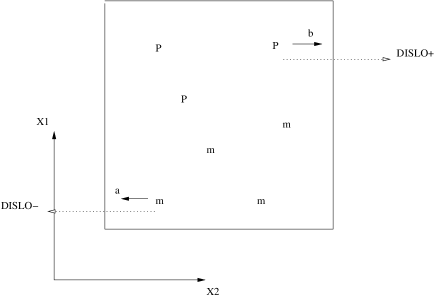
Figure 1: Groma-Balogh 2D model.

Here the velocity vector field is the shear stress in the material, solving the equations of elasticity. It turns out that this shear stress can be expressed as some Riesz transform of the solution (see Section 2). More precisely our non-linear and non-local system of transport equations is the following:

$$\left\{\begin{array}[]{lll}\displaystyle{\frac{\partial{\rho}^{+}}{\partial t}(x,t)}=-&\left(R_{1}^{2}R_{2}^{2}\left(\rho^{+}(\cdot,t)-\rho^{-}(\cdot,t)\right)(x)\right)\displaystyle{\frac{\partial{\rho}^{+}}{\partial x_{1}}(x,t)}&\mbox{in $\mathbb{{\cal D}}^{\prime}({\mathbb{R}}^{2}\times(0,T))$,}\\ \\ \displaystyle{\frac{\partial{\rho}^{-}}{\partial t}(x,t)}=&\left(R_{1}^{2}R_{2}^{2}\left(\rho^{+}(\cdot,t)-\rho^{-}(\cdot,t)\right)(x)\right)\displaystyle{\frac{\partial{\rho}^{-}}{\partial\par x_{1}}(x,t)}&\mbox{in $\mathbb{{\cal D}}^{\prime}({\mathbb{R}}^{2}\times(0,T))$.}\end{array}\right.$$ (P)

The unknowns of the system (P) are the scalar functions $\rho^{+}$ and $\rho^{-}$ at the time $t$ and the position $x=(x_{1},x_{2})$, that we denote for simplification by $\rho^{\pm}$. These terms correspond to the plastic deformations in a crystal. Their derivative in the $x_{1}$ direction (i.e. the direction of Burgers vector $\vec{b}$), $\displaystyle{\frac{\partial{\rho}^{\pm}}{\partial x_{1}}}$ represents the dislocation densities of $\pm$ type. In our work, we will only consider solutions ${\rho}^{\pm}$ such that $\displaystyle{\frac{\partial{\rho}^{\pm}}{\partial t}}$, $\nabla{\rho}^{\pm}$ and ${\rho}^{+}-{\rho}^{-}$ are ${\mathbb{Z}}^{2}$-periodic functions. The operators $R_{1}$ (resp. $R_{2}$) are the Riesz transformations associated to $x_{1}$ (resp. $x_{2}$). More precisely, these Riesz transforms are defined as follows:

Definition 1.1

(Riesz transform in the periodic case)
Let the torus $\mathbb{T}^{2}={\mathbb{R}}^{2}/{\mathbb{Z}}^{2}$. We define for $i\in\{1,2\}$ the Riesz transforms $R_{i}$ over $\mathbb{T}^{2}$ as follows. If $f\in L^{2}(\mathbb{T}^{2})$, the Fourier series coefficients of $R_{i}f$ are given by:

i) $c_{(0,0)}\left(R_{i}f\right)=0,$

ii) $c_{k}\left(R_{i}f\right)=\displaystyle{\frac{k_{i}}{|k|}}c_{k}(f)\;\;\;\mbox{for $k=(k_{1},k_{2})\in\mathbb{Z}^{2}\setminus\{(0,0)\},$}$

where we recall that $\displaystyle{c_{k}(f)=\int_{\mathbb{T}^{2}}f(x)e^{-2\pi ik\cdot x}d^{2}x}$.

In fact, this 2D model has been generalized later in 2003 by I. Groma, F. Csikor and M. Zaiser in a model taking into account the back stress describing more carefully boundary layers (see [24] for further details). The Groma-Balogh model neglects in particular the short range dislocation-dislocation correlations in one slip direction. For an extension to multiple slip see S. Yefimov and E. Van der Giessen [38, ch. 5.]. This multiple slip version of the Groma-Balogh model presents some analogies with some traffic flow models (see O. Biham et al. [8]). See also V. S. Deshpande et al. [14] for a similar model with boundary conditions and exterior forces. Recently, A. EL-Azab [16], M. Zaiser, T. Hochrainer [39] and R. Monneau [29] were interested in modeling the dynamics of dislocation densities in the three-dimensional space, but many more open questions have to be solved for establishing a satisfactory three-dimensional theory of dislocations dynamics and for getting rigorous results.

We stress out the attention of the reader that there was no existence and uniqueness results for (P). In this paper we prove that (P) admits a “global in time” solution.

1.2 Main result

In the present paper, we prove a “global in time” existence result for the system (P) describing the dynamics of dislocation densities.

In this work, we consider the following initial conditions:

$${\rho}^{\pm}(x_{1},x_{2},t=0)={\rho}^{\pm}_{0}(x_{1},x_{2})={\rho}^{\pm,per}_{0}(x_{1},x_{2})+Lx_{1},$$ (IC)

where ${\rho}^{\pm,per}$ is a $1$-periodic function in $x_{1}$ and $x_{2}$. The periodicity is a way of studying the bulk behavior of the material away from its boundary. Here $L$ is a given positive constant that represents the initial total dislocation densities of $\pm$ type on the periodic cell.

Before to give our main result, we want to show that the bilinear term on the right hand side of (P) is well defined. To this end, we need first to recall the following definition:

Definition 1.2

(The space $L\log L$)
We define the space $L\log L(\mathbb{T}^{2})$

$$L\log L(\mathbb{T}^{2})=\left\{\mbox{$f\in L^{1}(\mathbb{T}^{2})$ such that $\displaystyle{\int_{\mathbb{T}^{2}}|f|\ln\left(e+|f|\right)<+\infty}$}\right\}.$$

This space is endowed with the (Luxemburg) norm

$$\|f\|_{L\log L(\mathbb{T}^{2})}=\inf\left\{\lambda>0:\displaystyle{\int_{\mathbb{T}^{2}}}\frac{|f|}{\lambda}\ln\left(e+\frac{|f|}{\lambda}\right)\leq 1\right\}.$$

The space $L\log L(\mathbb{T}^{2})$ is a special space of Zygmund spaces (see R. A. Adams [1, (13), Page 234], E. M. Stein [36, Page 43])

We can now state the following proposition.

Proposition 1.3

(Meaning of the bilinear term)
Let $T>0$, $f$ and $g$ be two functions defined on $\mathbb{T}^{2}\times(0,T)$, such that
$f\in L^{1}((0,T);W^{1,2}(\mathbb{T}^{2}))$ and $g\in L^{\infty}((0,T);L\log L(\mathbb{T}^{2}))$ then,

$$fg\in L^{1}(\mathbb{T}^{2}\times(0,T)).$$

We will see that the proof of this proposition (given in Subsection 3.2) is a direct consequence of Trudinger inequality.

We can now state our main result (see also our comments in Subsection 1.3 on the unknown uniqueness of the solution).

Theorem 1.4

(Global existence)
For all $T,L>0$ , and for every initial data $\rho_{0}^{\pm}\in L^{2}_{loc}({\mathbb{R}}^{2})$ with

1. $\rho_{0}^{\pm}(x_{1}+1,x_{2})=\rho_{0}^{\pm}(x_{1},x_{2})+L,$ a.e. on ${\mathbb{R}}^{2}$,

2. $\rho_{0}^{\pm}(x_{1},x_{2}+1)=\rho_{0}^{\pm}(x_{1},x_{2}),$ a.e. on ${\mathbb{R}}^{2}$,

3. $\displaystyle{\frac{\partial{\rho_{0}}^{\pm}}{\partial x_{1}}}\geq 0,$ a.e. on ${\mathbb{R}}^{2}$,

4. $\left\|\displaystyle{\frac{\partial{\rho_{0}}^{\pm}}{\partial x_{1}}}\right\|_{L\log L(\mathbb{T}^{2})}\leq C$, with $\mathbb{T}^{2}={\mathbb{R}}^{2}/{\mathbb{Z}}^{2}$,

the system (P)-(IC) admits solutions $\rho^{\pm}\in C([0,T);L^{1}_{loc}({\mathbb{R}}^{2}))\cap L^{\infty}((0,T);L^{2}_{loc}({\mathbb{R}}^{2}))$ in the distributional sense, such that, $\rho^{\pm}(\cdot,t)$ satisfy $(H1)$, $(H2)$, $(H3)$ and $(H4)$ for a.e. $t\in(0,T)$. Moreover, we have:

1. $R_{1}^{2}R_{2}^{2}\left(\rho^{+}-\rho^{-}\right)\in L^{2}((0,T);W^{1,2}_{loc}({\mathbb{R}}^{2})).$

Remark 1.5

(Bilinear term)
It is clear here that the bilinear term on the right hand side of(P) is always defined via $(P1)$ and Proposition 1.3.

In order to prove our main theorem we regularize the system (P) by adding the viscosity term ($\varepsilon\Delta\rho^{\pm}$), and regularized also the initial data (IC) by classical convolution. Then, using a fixed point Theorem, we prove that our regularized system admits local in time solutions. Moreover, as we get some $\varepsilon$-independent a priori estimates we will be able to extend our local in time solution into a global one. This turns out to be possible thanks to the entropy inequality (1.1). Then, joined with other a priori estimates, it will be possible to prove some compactness properties and to pass to the limit as $\varepsilon$ goes to $0$ is the $\varepsilon$-problem.

Remark 1.6

(Entropy and energy inequalities)
It turns out that the constructed solution also satisfies the following fundamental entropy inequality (as a consequence of Lemma 5.4), for a.e. $t\in(0,T)$,

$$\begin{array}[]{ll}\displaystyle{\int_{\mathbb{T}^{2}}}\sum_{\pm}\displaystyle{\frac{\partial{\rho}^{\pm}}{\partial x_{1}}}\ln\left(\displaystyle{\frac{\partial{\rho}^{\pm}}{\partial x_{1}}}\right)+\displaystyle{\int_{0}^{t}}\int_{\mathbb{T}^{2}}\left(R_{1}R_{2}\left(\displaystyle{\frac{\partial{\rho}^{+}}{\partial x_{1}}}-\displaystyle{\frac{\partial{\rho}^{-}}{\partial x_{1}}}\right)\right)^{2}\leq\displaystyle{\int_{\mathbb{T}^{2}}\sum_{\pm}\displaystyle{\frac{\partial{\rho}^{\pm}_{0}}{\partial x_{1}}}\ln\left(\displaystyle{\frac{\partial{\rho}_{0}^{\pm}}{\partial x_{1}}}\right)}\end{array}$$ (1.1)

Moreover, (at least formally for sufficiently regular solution) the following energy inequality holds:

$$\begin{array}[]{ll}\displaystyle{\frac{1}{2}\int_{\mathbb{T}^{2}}\left(R_{1}R_{2}(\rho^{+}-\rho^{-})(\cdot,t)\right)^{2}}&+\displaystyle{\int_{0}^{t}\int_{\mathbb{T}^{2}}\left(R_{1}^{2}R_{2}^{2}(\rho^{+}-\rho^{-})\right)^{2}\left(\displaystyle{\frac{\partial{\rho}^{+}}{\partial x_{1}}}+\displaystyle{\frac{\partial{\rho}^{-}}{\partial x_{1}}}\right)}\leq\\ &\displaystyle{\frac{1}{2}\int_{\mathbb{T}^{2}}\left(R_{1}R_{2}(\rho^{+}_{0}-\rho^{-}_{0})\right)^{2}}\end{array}$$

Remark 1.7

(Bounds on the solution)
If we denote $\rho=\rho^{+}-\rho^{-}$, then there exists a constant $C$ independent on $T$, and a constant $C_{T}$ depending on $T$ such that,

$(E1)$ $\|\rho^{\pm}-Lx_{1}\|_{L^{\infty}((0,T);L^{2}(\mathbb{T}^{2}))}\leq C_{T},$            $(E4)$ $\|R_{1}^{2}R_{2}^{2}\rho\|_{L^{2}((0,T);W^{1,2}(\mathbb{T}^{2}))}\leq C,$

$(E2)$ $\left\|\displaystyle{\frac{\partial{\rho}^{\pm}}{\partial x_{1}}}\right\|_{L^{\infty}((0,T);L\log L(\mathbb{T}^{2}))}\leq C,$                $(E5)$ $\left\|\displaystyle{R_{1}^{2}R_{2}^{2}\frac{\partial{\rho}}{\partial t}}\right\|_{L^{2}((0,T);W^{-1,2}(\mathbb{T}^{2}))}\leq C,$

$(E3)$ $\left\|\displaystyle{\frac{\partial{\rho}^{\pm}}{\partial t}}\right\|_{L^{2}((0,T);L^{1}(\mathbb{T}^{2}))}\leq C,$

where $W^{-1,2}(\mathbb{T}^{2})$ is the dual space of $W^{1,2}(\mathbb{T}^{2})$.

In a particular sub-case of model (P) where the dislocation densities depend on a single variable $x=x_{1}+x_{2}$, the existence and uniqueness of a Lipschitz viscosity solution was proved in A. El Hajj, N. Forcadel [18]. Also the existence and uniqueness of a strong solution in $W^{1,2}_{loc}({\mathbb{R}}\times[0,T))$ was proved in A. El Hajj [17]. Concerning the model of I. Groma, F. Csikor, M. Zaiser [24] which takes into consideration the short range dislocation-dislocation correlations giving a parabolic-hyperbolic system, let us mention the work of H. Ibrahim [26] where a result of existence and uniqueness of a viscosity solution is given but only for a one-dimensional model.

Our study of the dynamics of dislocation densities in a special geometry is related to the more general dynamics of dislocation lines. We refer the interested reader to the work of O. Alvarez et al. [3], for a local existence and uniqueness of some non-local Hamilton-Jacobi equation. We also refer to O. Alvarez et al. [2] and G. Barles, O. Ley [6] for some long time existence results.

1.3 Comments on the uniqueness of the solution and related literature

The problem (P) is a system of transport equations with low regularity of the vector field, so that the uniqueness of the solution here is an open question. However, in the following we present some uniqueness results where the vector field has a better regularity.

From a technical point of view, (P) is related to other well known models, such as the transport equation with a low regularity vector field. This equation was studied in the work of R. J. Diperna, P. L. Lions [15] and L. Ambrosio [4], where the authors showed the existence and uniqueness of renormalized solutions by considering vector fields in $L^{1}((0,T);W^{1,1}_{loc}({\mathbb{R}}^{N}))$ and $L^{1}((0,T);BV_{loc}({\mathbb{R}}^{N}))$ respectively in both cases with bounded divergence. On the contrary in system (P), we are only able to prove that for the constructed solution, the vector field is in $L^{2}((0,T);W^{1,2}_{loc}({\mathbb{R}}^{2}))$ without any better estimate on the divergence of the vector field.

More generally in the frame of symmetric hyperbolic systems, we refer to the book of D. Serre [34, Vol I, Th 3.6.1], for a typical result of local existence and uniqueness in $C([0,T);H^{s}({\mathbb{R}}^{N}))\cap C^{1}([0,T);H^{s-1}({\mathbb{R}}^{N}))$, with $s>\frac{N}{2}+1$, by considering initial data in $H^{s}({\mathbb{R}}^{N})$. This result remains local in time, even in dimension $N=2$.

We can also remark that in the case where we multiply the right side of the two equations in system (P) by $-1$, we get a quasi-geostrophic-like system. For those who are concerned in quasi-geostrophic systems, we refer to P. Constantin et al. [11], and to [12] for certain 2D numerical results. We also refer to A. Córdoba, D. Córdoba [13], D. Chae, A. Córdoba [10] for blow-up results in finite time, in dimension one.

Let us also mention some related Vlasov-Poisson models (see J. Nieto et al. [30] for instance) and a related model in superconductivity studied by N. Masmoudi et al. [28] and by L. Ambrosio et al. [5]. These models were derived from some Vlasov-Poisson-Fokker-Planck models (see for instance T. Goudon et al. [21] for an overview of similar models). It is also worth mentioning that this model is related to Vlasov-Navier-Stokes equation see T. Goudon et al. [19], [20].

1.4 Notation

In what follows, we are going to use the following notation:

1. $\rho=\rho^{+}-\rho^{-}$,

2. $\rho^{\pm,per}(x_{1},x_{2},t)=\rho^{\pm}(x_{1},x_{2},t)-Lx_{1}$,

3. Let $f$ be a function defined on ${\mathbb{R}}^{2}\times(0,T)$ having values in ${\mathbb{R}}^{2}$, we denote by $f(t)=f(.,t):x\longmapsto f(x,t)$,

4. Throughout the paper, $C$ is an arbitrary positive constant independent on $T$ and $C_{T}$ is an arbitrary positive constant depending on $T$.

1.5 Organization of the paper

First, in Section 2, we recall the physical derivation of system (P). In Section 3, we recall the definitions and properties of some useful fundamental spaces, and we give the proof of Proposition 1.3. We also prove that the bilinear term of our system has a better mathematical meaning (see Proposition 3.4). Next, in Section 4, we regularize the initial conditions and we show that the system (P), modified by a term ($\varepsilon\displaystyle{\Delta\rho^{\pm}}$), admits local solutions. Moreover, we show that these solutions are regular and increasing for all $t\in(0,T)$, for increasing initial data. In Section 5, we prove some $\varepsilon$-uniform a priori estimates for the regularized solution obtained in Section 4. Then, thanks to these a priori estimates, we extend the local in time solutions for the $\varepsilon$-problem constructed in Section 4, in to global in time solution. Finally, in Section 6, we achieve the proof of our main theorem, passing to the limit in the equation as $\varepsilon$ goes to $0$, and using some compactness properties inherited from our a priori estimates.

2 Physical derivation of the model

In this section we explain how to derive physically the system (P). We consider a three-dimensional crystal, with displacement

$$u=(u_{1},u_{2},u_{3}):{\mathbb{R}}^{3}\rightarrow{\mathbb{R}}^{3}.$$

For $x=(x_{1},x_{2},x_{3})$, and an orthogonal basis $(e_{1},e_{2},e_{3})$, we define the total strain by:

$${\varepsilon_{ij}(u)=\frac{1}{2}}\left(\displaystyle{\frac{\partial u_{i}}{\partial{x_{j}}}}+\displaystyle{\frac{\partial u_{j}}{\partial{x_{i}}}}\right),\;\;\;i,j=1,2,3.$$

This total strain is decomposed as

$$\varepsilon_{ij}(u)=\varepsilon^{e}_{ij}+\varepsilon^{p}_{ij},$$

with $\varepsilon^{e}_{ij}$ is the elastic strain and $\varepsilon^{p}_{ij}$ the plastic strain which is defined by:

$$\varepsilon^{p}_{ij}=\rho\varepsilon^{0}_{ij},$$ (2.2)

with the fixed matrix $\displaystyle{\varepsilon^{0}_{ij}=\frac{1}{2}\left(1-\delta_{ij}\right)}$, where $\delta_{ij}$ is the Kronecker symbol, in the special case of a single slip system where dislocations move in the plane $\{x_{2}=0\}$ with Burgers vector $\vec{b}=e_{1}$. Here $\gamma$ is the resolved plastic strain, and will be clarified later. In the case of linear homogeneous and isotropic elasticity, the stress is given by

$${\sigma_{ij}=2\mu\varepsilon^{e}_{ij}+\lambda\delta_{ij}\left(\sum_{k=1,2,3}\varepsilon^{e}_{kk}\right)}\;\;\;\;\mbox{for $i,j=1,2,3$,}$$ (2.3)

where $\lambda,\mu$ are the constant Lam coefficients of the crystal (satisfying $\mu>0$ and $3\lambda+2\mu>0$). Moreover the stress satisfies the equation of elasticity:

$${\sum_{j=1,2,3}\frac{\partial\sigma_{ij}}{\partial{x_{j}}}}=0.$$

We now assume that we are in a particular geometry where the dislocations are straight lines parallel to the direction $e_{3}$ and that the problem is invariant by translation in the $x_{3}$ direction. Moreover we assume that $u_{3}=0$ and $\sigma_{i3}=0$ for $i=1,2,3$. Then, this problem reduces to a two-dimensional problem with $u_{1},u_{2}$ only depending on $(x_{1},x_{2})$ and so we can express the resolved plastic strain $\rho$ as

$$\rho=\rho^{+}-\rho^{-},$$

where $\displaystyle{\frac{\partial\rho^{+}}{\partial{x_{1}}}}$ and $\displaystyle{\frac{\partial\rho^{-}}{\partial{x_{1}}}}$ are respectively the densities of dislocations of Burgers vectors given by $\vec{b}=e_{1}$ and $\vec{b}=-e_{1}$.

Furthermore, these dislocation densities are transported in the direction of the Burgers vector at a given velocity. This velocity is indeed the resolved shear stress $\displaystyle{\sum_{i,j=1,2,3}\sigma_{ij}\varepsilon^{0}_{ij}=\sigma_{12}}$, up to sign of the Burgers vectors. More precisely, we have:

$${\frac{\partial\rho^{\pm}}{\partial t}}=\pm(\sigma_{12})\displaystyle{e_{1}.\nabla\rho^{\pm}}.$$

Finally, the functions $\rho^{\pm}$ and $u=(u_{1},u_{2})$ are solutions of the coupled system (see I. Groma, P. Balogh [23], [22]), on ${\mathbb{R}}^{2}\times(0,T)$:

$$\left\{\begin{array}[]{lll}\displaystyle{\sum_{j=1,2}\frac{\partial\sigma_{ij}}{\partial x_{j}}}&=0&\mbox{for $i=1,2$,}\\ \sigma_{ij}&=\displaystyle{2\mu\varepsilon^{e}_{ij}+\lambda\delta_{ij}\left(\sum_{k=1,2}\varepsilon^{e}_{kk}\right)}&\mbox{for $i,j=1,2$,}\\ \varepsilon_{ij}^{e}&=\displaystyle{\frac{1}{2}}\left(\displaystyle{\frac{\partial u_{i}}{\partial{x_{j}}}}+\displaystyle{\frac{\partial u_{j}}{\partial{x_{i}}}}\right)-(\rho^{+}-{\rho}^{-})\varepsilon_{ij}^{0}&\mbox{for $i,j=1,2$,}\\ \varepsilon_{ij}^{0}&=\displaystyle{\frac{1}{2}}\left(1-\delta_{ij}\right)&\mbox{for $i,j=1,2$,}\\ $\;$\\ \displaystyle{\frac{\partial\rho^{\pm}}{\partial t}}&=\pm\sigma_{12}\displaystyle{\frac{\partial\rho^{\pm}}{\partial x_{1}}}.\end{array}\right.$$ (2.4)

Then the following lemma holds.

Lemma 2.1

(Computation of $\sigma_{12}$)
Assume that $(u_{1},u_{2})$ and $\rho=\rho^{+}-\rho^{-}$ are ${\mathbb{Z}}^{2}$-periodic functions. If $(u_{1},u_{2})$, $\rho^{+}$, $\rho^{-}$ are solutions of problem (2.4), then

$$\sigma_{12}=-C_{1}\left(R_{1}^{2}R_{2}^{2}\rho\right),$$ (2.5)

where $\displaystyle{C_{1}=4\frac{(\lambda+\mu)\mu}{\lambda+2\mu}}>0$.

Using this expression of $\sigma_{12}$ and rescaling in time with the positive constant $C_{1}$ we obtain system (P), from the last equation (2.4).

Proof of Lemma 2.1:
We can rewrite the first equation of (2.4) with $\hbox{div}\;u=\displaystyle{\frac{\partial u_{1}}{\partial{x_{1}}}}+\displaystyle{\frac{\partial u_{2}}{\partial{x_{2}}}}$

$$\mu\Delta u_{1}+(\lambda+\mu)\displaystyle{\frac{\partial}{\partial{x_{1}}}}(\hbox{div}\;u)=\mu\displaystyle{\frac{\partial\rho}{\partial{x_{2}}}},$$ (2.6a)

$$\mu\Delta u_{2}+(\lambda+\mu)\displaystyle{\frac{\partial}{\partial{x_{2}}}}(\hbox{div}\;u)=\mu\displaystyle{\frac{\partial\rho}{\partial{x_{1}}}}.$$ (2.6b)

Considering $\displaystyle{\frac{\partial}{\partial{x_{1}}}}$(2.6a)+$\displaystyle{\frac{\partial}{\partial{x_{2}}}}$(2.6b), we get

$${(\lambda+2\mu)\Delta(\hbox{div}\;u)=2\mu\frac{\partial^{2}\rho}{\partial{x_{1}}\partial{x_{2}}}}.$$

Plugging the expression of $\hbox{div}\;u$ into (2.6), we get

$$\Delta u_{1}=\displaystyle{\frac{\partial\rho}{\partial{x_{2}}}}-2\frac{(\lambda+\mu)}{(\lambda+2\mu)}\displaystyle{\frac{\partial}{\partial{x_{1}}}}\Delta^{-1}\displaystyle{\frac{\partial^{2}\rho}{\partial{x_{1}}\partial{x_{2}}}},$$ (2.7a)

$$\Delta u_{2}=\displaystyle{\frac{\partial\rho}{\partial{x_{1}}}}-2\frac{(\lambda+\mu)}{(\lambda+2\mu)}\displaystyle{\frac{\partial}{\partial{x_{2}}}}\Delta^{-1}\displaystyle{\frac{\partial^{2}\rho}{\partial{x_{1}}\partial{x_{2}}}}.$$ (2.7b)

Considering now $\displaystyle{\frac{\partial}{\partial{x_{2}}}}$(2.7a)+$\displaystyle{\frac{\partial}{\partial{x_{1}}}}$(2.7b) , we obtain

$$\Delta\left(\displaystyle{\frac{\partial u_{1}}{\partial{x_{2}}}}+\displaystyle{\frac{\partial u_{2}}{\partial{x_{1}}}}\right)=\Delta(\rho^{+}-\rho^{-})-4\frac{(\lambda+\mu)}{(\lambda+2\mu)}\Delta^{-1}\displaystyle{\frac{\partial^{4}}{\partial{x_{1}^{2}}\partial{x_{2}^{2}}}(\rho^{+}-\rho^{-})}.$$ (2.8)

Recalling that

$$\sigma_{12}=\mu\left(\displaystyle{\left(\displaystyle{\frac{\partial u_{1}}{\partial{x_{2}}}}+\displaystyle{\frac{\partial u_{2}}{\partial{x_{1}}}}\right)-(\rho^{+}-\rho^{-})}\right),$$ (2.9)

this yields $\sigma_{12}=-4\frac{(\lambda+\mu)\mu}{(\lambda+2\mu)}\Delta^{-2}\displaystyle{\frac{\partial^{4}}{\partial{x_{1}^{2}}\partial{x_{2}^{2}}}(\rho^{+}-\rho^{-})}=-C_{1}\left(R_{1}^{2}R_{2}^{2}(\rho^{+}-\rho^{-})\right).$ $\hfill\Box$

Remark 2.2

(Property of the elastic energy)
If we define the elastic energy by

$${E=\int_{{\mathbb{R}}^{2}/{\mathbb{Z}}^{2}}\mu\sum_{i,j=1,2}(\varepsilon_{ij}^{e})^{2}+\frac{\lambda}{2}\left(\sum_{k=1,2}\varepsilon_{kk}^{e}\right)^{2}.}$$

Using system (2.4) we can show formally that

$${\frac{dE}{dt}}=-\int_{{\mathbb{R}}^{2}/{\mathbb{Z}}^{2}}(\sigma_{12})^{2}\left(\displaystyle{\frac{\partial\rho^{+}}{\partial{x_{1}}}}+\displaystyle{\frac{\partial\rho^{-}}{\partial{x_{1}}}}\right)\leq 0.$$

where we have used the fact that $\displaystyle{\frac{\partial\rho^{+}}{\partial{x_{1}}}},\displaystyle{\frac{\partial\rho^{-}}{\partial{x_{1}}}}\geq 0$ to see that the elastic energy is a non-increasing in time. Hence, the elastic energy $E$ is a Lyapunov functional for our dissipative model.

3 Concerning the meaning of the solution of (P)

In this section we prove Proposition 1.3. This shows that if (P) admits solutions verifying the conditions of Theorem 1.4, then we can give a mathematical meaning to the bilinear term. In order to do this, we need to define some functional spaces and recall some of their properties, that will be used later in our work.

3.1 Properties of some useful Orlicz spaces

We recall the definition of Orlicz spaces and some of their properties. For details, we refer to R. A. Adams [1, Ch. 8] and M. M. Rao, Z. D. Ren [33].

A real valued function $\displaystyle{A:[0,+\infty)\rightarrow{\mathbb{R}}}$ is called a Young function if it has the following properties (see R. O’Neil [31, Def 1.1]):

• $A$ is a continuous, non-negative, non-decreasing and convex function.

• $A(0)=0$ and $\displaystyle{\lim_{t\rightarrow+\infty}A(t)=+\infty}$.

Let $A(\cdot)$ be a Young function. The Orlicz class $K_{A}(\mathbb{T}^{2})$ is the set of (equivalence classes of) real-valued measurable function $h$ on $\mathbb{T}^{2}$ satisfying

$${\int_{\mathbb{T}^{2}}A(|h(x)|)<+\infty}.$$

The Orlicz space $L_{A}(\mathbb{T}^{2})$ is the linear hull of $K_{A}(\mathbb{T}^{2})$ supplemented with the Luxemburg norm

$$\|f\|_{L_{A}(\mathbb{T}^{2})}=\inf\left\{\lambda>0:\displaystyle{\int_{\mathbb{T}^{2}}}A\left(\frac{|h(x)|}{\lambda}\right)\leq 1\right\}.$$

Endowed with this norm, the Orlicz space $L_{A}(\mathbb{T}^{2})$ is a Banach space. Moreover, for all $f\in L_{A}(\mathbb{T}^{2})$, we have the following estimate

$$\|f\|_{L_{A}(\mathbb{T}^{2})}\leq 1+\int_{\mathbb{T}^{2}}A(|f(x)|)$$ (3.10)

Definition 3.1

(Some Orlicz spaces)

$\bullet\;\;\mbox{$EXP_{\alpha}(\mathbb{T}^{2})$ denotes the Orlicz space defined by the function $A(t)=e^{t^{\alpha}}-1$ for $\alpha\geq 1$}.$

$\bullet\;\;\mbox{$L\log^{\beta}L(\mathbb{T}^{2})$ denotes the Orlicz space defined by the function $A(t)=t(\log(e+t))^{\beta}$, for $\beta\geq 0$}.$

Observe that for $0<\beta\leq 1$ the space $EXP_{\frac{1}{\beta}}(\mathbb{T}^{2})$ is the dual of the Zygmund space $L\log^{\beta}L(\mathbb{T}^{2})$. (see C. Bennett and R. Sharpley [7, Def 6.11]). It is worth noticing that $L\log^{1}L(\mathbb{T}^{2})=L\log L(\mathbb{T}^{2})$.

Let us recall some useful properties of these spaces. The first one is the generalized H lder inequality.

Lemma 3.2

(Generalized H lder inequality)
i) Let $f\in EXP_{2}(\mathbb{T}^{2})$ and $g\in L\log^{\frac{1}{2}}L(\mathbb{T}^{2})$. Then there exists a constant $C$ such that (see R. O’Neil [31, Th 2.3])

$$\|fg\|_{L^{1}(\mathbb{T}^{2})}\leq C\|f\|_{EXP_{2}(\mathbb{T}^{2})}\|g\|_{L\log^{\frac{1}{2}}L(\mathbb{T}^{2})}.$$

ii) Let $f\in EXP_{2}(\mathbb{T}^{2})$ and $g\in L\log L(\mathbb{T}^{2})$. Then there exists a constant $C$ such that (see R. O’Neil [31, Th 2.3])

$$\|fg\|_{L\log^{\frac{1}{2}}L(\mathbb{T}^{2})}\leq C\|f\|_{EXP_{2}(\mathbb{T}^{2})}\|g\|_{L\log L(\mathbb{T}^{2})}.$$

The second property is the Trudinger inequality.

Lemma 3.3

(Trudinger inequality)
There exists a constant $\gamma>0$ such that, for all $f\in W^{1,2}(\mathbb{T}^{2})$, we have (see N. S. Trudinger [37])

$${\int_{\mathbb{T}^{2}}\displaystyle{e}^{\displaystyle{\gamma}\left(\displaystyle{\frac{f}{\|f\|_{W^{1,2}(\mathbb{T}^{2})}}}\right)^{2}}}\leq 1.$$

In particular we have the following embedding

$$W^{1,2}(\mathbb{T}^{2})\hookrightarrow EXP_{2}(\mathbb{T}^{2}).$$

3.2 Sharp estimate of the bilinear term

Now, we propose to verify with the help of the following proposition that the system (P) has indeed a sense, and first prove a better estimate than those mentioned in Proposition 1.3. Namely, we have the following.

Proposition 3.4

(Estimate of the bilinear term)
Let $T>0$, $f$ and $g$ be two functions defined on $\mathbb{T}^{2}\times(0,T)$, such that

1. $f\in L^{2}((0,T);W^{1,2}(\mathbb{T}^{2}))$,

2. $g\in L^{\infty}((0,T);L\log L(\mathbb{T}^{2}))$. Then

$$fg\in L^{2}((0,T);L\log^{\frac{1}{2}}L(\mathbb{T}^{2}))$$

and for a positive constant $C$, we have:

$$\|fg\|_{L^{2}((0,T);L\log^{\frac{1}{2}}L(\mathbb{T}^{2}))}\leq C\|f\|_{L^{2}((0,T);W^{1,2}(\mathbb{T}^{2}))}\|g\|_{L^{\infty}((0,T);L\log L(\mathbb{T}^{2}))}.$$

For the proof of this Proposition , we use Lemma 3.2 (ii), and integrate in time. Thanks to the Trudinger inequality (Lemma 3.3), we get the result. We do the same way for the proof of the Proposition 1.3.

4 Local existence of solutions of a regularized system

In this section, we state a local in time existence result for system (P), modified by the term $\varepsilon\Delta\rho^{\pm}$, and for smoothed data. This modification brings us to study, for all $0<\varepsilon\leq 1$, the following regularized system:

$$\left\{\begin{array}[]{lll}\displaystyle{\frac{\partial{\rho}^{+,\varepsilon}}{\partial t}}-\varepsilon\Delta{\rho}^{+,\varepsilon}&=-(R_{1}^{2}R_{2}^{2}\rho^{\varepsilon})\displaystyle{\frac{\partial{\rho}^{+,\varepsilon}}{\partial x_{1}}}&\mbox{in $\mathbb{{\cal D}}^{\prime}({\mathbb{R}}^{2}\times(0,T))$,}\\ \\ \displaystyle{\frac{\partial{\rho}^{-,\varepsilon}}{\partial t}}-\varepsilon\Delta{\rho}^{-,\varepsilon}&=\;\;\;(R_{1}^{2}R_{2}^{2}\rho^{\varepsilon})\displaystyle{\frac{\partial{\rho}^{-,\varepsilon}}{\partial x_{1}}}&\mbox{in $\mathbb{{\cal D}}^{\prime}({\mathbb{R}}^{2}\times(0,T))$,}\\ \end{array}\right. P_{\varepsilon}$$ ()

where $\rho^{\varepsilon}=\rho^{+,\varepsilon}-\rho^{-,\varepsilon}$, with the following regular initial data:

$$\rho^{\pm,\varepsilon}(x,0)=\rho_{0}^{\pm,\varepsilon}(x)=\rho^{\pm,per}_{0}\ast\eta_{\varepsilon}(x)+(L+\varepsilon)x_{1}=\rho^{\pm,\varepsilon,per}_{0}(x)+L_{\varepsilon}x_{1}, IC_{\varepsilon}$$ ()

where $\eta_{\varepsilon}(\cdot)=\frac{1}{\varepsilon^{2}}\eta(\frac{\cdot}{\varepsilon})$, such that $\eta\in C^{\infty}_{c}({\mathbb{R}}^{2})$ is a non-negative function and $\int_{{\mathbb{R}}^{2}}\eta=1$.

Remark 4.1

 
We consider $L_{\varepsilon}=L+\varepsilon$ to obtain strictly monotonous initial data $\rho_{0}^{\pm,\varepsilon}$. This condition will be useful in the proof of Lemma 5.4.

For the regularized system ($P_{\varepsilon}$)-($IC_{\varepsilon}$) we have the following result.

Theorem 4.2

(Local existence result of monotone smooth solutions)
For all initial data $\rho^{\pm}_{0}\in L^{2}_{loc}({\mathbb{R}}^{2})$ satisfying $(H1)$, $(H2)$ and $(H3)$, and all $\varepsilon>0$, there exists $T^{\star}>0$ such that the system ($P_{\varepsilon}$)-($IC_{\varepsilon}$) admits solutions $\rho^{\pm,\varepsilon}\in C^{\infty}({\mathbb{R}}^{2}\times[0,T^{\star}))$. Moreover $\rho^{\pm,\varepsilon}(\cdot,t)$ satisfy $(H1)$, $(H2)$ and $\displaystyle{\frac{\partial\rho^{\pm,\varepsilon}}{\partial x_{1}}>0}$, for all $t\in[0,T^{\star})$.

Before proving Theorem 4.2, let us recall some well known results.

We first recall the Picard fixed point result which will be applied in the proof of this theorem in order to prove, the existence of solutions.

Lemma 4.3

(Picard Fixed point Theorem)
Let $E$ be a Banach space, $B$ is a continuous bilinear application over $E\times E$ having values in $E$, and $A$ a continuous linear application over $E$ having values in $E$ such that:

$$\|B(x,y)\|_{E}\leq\eta\|x\|_{E}\|y\|_{E}\;\;\;\mbox{for all}\;\;\;x,y\in E,$$

$$\|A(x)\|_{E}\leq\mu\|x\|_{E}\;\;\;\mbox{for all}\;\;\;x\in E,$$

where $\eta>0$ and $\mu\in(0,1)$ are two given constants. Then, for every $x_{0}\in E$ verifying

$$\|x_{0}\|_{E}<\frac{1}{4\eta}(1-\mu)^{2},$$

the equation $x=x_{0}+B(x,x)+A(x)$ admits a solution in $E$.

For the proof of Lemma 4.3, see M. Cannone [9, Lemma 4.2.14].

We now recall the following decay estimates for the heat semi-group.

Lemma 4.4

(Decay estimate)
Let $r,p,q\geq 1$. Then, for all functions $f\in L^{q}(\mathbb{T}^{2})$ and $g\in L^{p}(\mathbb{T}^{2})$, where $\displaystyle{\frac{1}{r}\leq\frac{1}{q}+\frac{1}{p}}$, we have, for $S_{1}(t)=e^{t\Delta}$, the following estimates:

$i)\;\;\;\|S_{1}(t)(fg)\|_{L^{r}(\mathbb{T}^{2})}\leq Ct^{-\left(\frac{1}{p}+\frac{1}{q}-\frac{1}{r}\right)}\|f\|_{L^{q}(\mathbb{T}^{2})}\|g\|_{L^{p}(\mathbb{T}^{2})}\;\;\mbox{for all $t>0$,}$

$ii)\;\;\;\|\nabla S_{1}(t)(fg)\|_{L^{r}(\mathbb{T}^{2})}\leq Ct^{-\left(\frac{1}{2}+\frac{1}{p}+\frac{1}{q}-\frac{1}{r}\right)}\|f\|_{L^{q}(\mathbb{T}^{2})}\|g\|_{L^{p}(\mathbb{T}^{2})}\;\;\mbox{for all $t>0$,}$

where $C$ is a positive constant depending only on $r,p,q$.

The proof of this lemma is a direct application of the classical version of the $L^{r}$-$L^{p}$ estimates for the heat semi-group (see A. Pazy [32, Lemma 1.1.8, Th 6.4.5]) and the H lder inequality.

Here is now, the demonstration of Theorem 4.2.

Proof of Theorem 4.2:
Frist we prove using Lemma 4.3 the local existence of the regularized system ($P_{\varepsilon}$)-($IC_{\varepsilon}$). This result is achieved in a super-critical space. Here particularly we chose the space of functions $L^{\infty}((0,T);W^{1,\frac{3}{2}}_{loc}({\mathbb{R}}^{2}))$. The notation "super-critical space" is to say that we are choosing a space where our $\varepsilon$-problem is well defined, and where the right hand term (the bilinear term) is in a space better than $L^{1}$. This premits to use a bootstrap arguments which easily leads to the existence of smooth solution of the regularized problem.

Now, we note that, if we let $\rho^{\pm,\varepsilon,per}=\rho^{\pm,\varepsilon}-L_{\varepsilon}x_{1}$, we know that the system ($P_{\varepsilon}$) is equivalent to,

$${\frac{\partial{\rho}^{\pm,\varepsilon}}{\partial t}}-\varepsilon\Delta\rho^{\pm,\varepsilon,per}=\mp(R_{1}^{2}R_{2}^{2}\rho^{\varepsilon})\displaystyle{\frac{\partial{\rho}}{\partial x_{1}}^{\pm,\varepsilon,per}}\mp L_{\varepsilon}(R_{1}^{2}R_{2}^{2}\rho^{\varepsilon})\;\;\mbox{in ${\cal D}^{\prime}(\mathbb{T}^{2}\times(0,T))$,} P_{\varepsilon}^{per}$$ ()

with initial conditions,

$$\rho^{\pm,\varepsilon,per}(x,0)=\rho_{0}^{\pm,\varepsilon}(x)-L_{\varepsilon}x_{1}=\rho_{0}^{\pm,\varepsilon,per}(x). IC_{\varepsilon}^{per}$$ ()

To solve this system in the space $L^{\infty}((0,T);W^{1,\frac{3}{2}}(\mathbb{T}^{2}))$ we reduce to construct a solution $\rho^{\pm,\varepsilon,per}$ to the following integral problem (see A. Pazy [32, Th 5.2, Page 146])

$$\begin{array}[]{ll}\displaystyle{\rho^{\pm,\varepsilon,per}(\cdot,t)}=S_{\varepsilon}(t)\rho^{\pm,\varepsilon,per}_{0}&\mp L_{\varepsilon}\displaystyle{\int_{0}^{t}}S_{\varepsilon}(t-s)\left(R^{2}_{1}R^{2}_{2}\rho^{\varepsilon}(s)\right)ds\\ \\ &\mp\displaystyle{\int_{0}^{t}}S_{\varepsilon}(t-s)\left(\left(R^{2}_{1}R^{2}_{2}\rho^{\varepsilon}(s)\right)\displaystyle{\frac{\partial{\rho}}{\partial x_{1}}^{\pm,\varepsilon,per}(s)}\right)ds,\end{array} In_{\varepsilon}$$ ()

where $S_{\varepsilon}(t)=S_{1}(\varepsilon t)$, and $S_{1}(t)=e^{t\Delta}$ is a the heat semi-group. We rewrite the system ($In_{\varepsilon}$) in t he following vectorial form:

$${\rho_{v}^{\varepsilon}(x,t)}=S_{\varepsilon}(t)\rho_{0,v}^{\varepsilon}+L_{\varepsilon}\bar{J_{1}}\displaystyle{\int_{0}^{t}}S_{\varepsilon}(t-s)\left(R^{2}_{1}R^{2}_{2}\rho^{\varepsilon}(s)\right)ds+\bar{I_{1}}\displaystyle{\int_{0}^{t}}S_{\varepsilon}(t-s)\left(R^{2}_{1}R^{2}_{2}\rho^{\varepsilon}(s)\right)\displaystyle{\frac{\partial{\rho_{v}^{\varepsilon}}}{\partial x_{1}}(s)}ds,$$

where $S_{\varepsilon}(t)=S_{1}(\varepsilon t)$, $\rho_{v}^{\varepsilon}=(\rho^{+,\varepsilon,per},\rho^{-,\varepsilon,per})$, $\rho_{0,v}^{\varepsilon}=(\rho^{+,\varepsilon,per}_{0},\rho^{-,\varepsilon,per}_{0})$, $\bar{I_{1}}=\left(\begin{array}[]{cc}-1&0\\ 0&1\end{array}\right)$ and $\bar{J_{1}}=\left(\begin{array}[]{c}-1\\ 1\end{array}\right)$.

Which is equivalent to,

$${\rho_{v}^{\varepsilon}(x,t)}=S_{\varepsilon}(t)\rho_{0,v}^{\varepsilon}+B(\rho_{v}^{\varepsilon},\rho_{v}^{\varepsilon})(t)+A(\rho_{v}^{\varepsilon})(t),$$ (4.11)

where $B$ is a bilinear map and $A$ is a linear one defined respectively, for every vector $u=(u_{1},u_{2})$ and $v=(v_{1},v_{2})$, as follows:

$${B(u,v)(t)}=\bar{I_{1}}\int_{0}^{t}S_{\varepsilon}(t-s)\left(\left(R^{2}_{1}R^{2}_{2}(u_{1}-u_{2})\right)\displaystyle{\frac{\partial{v}}{\partial x_{1}}(s)}\right)ds,$$ (4.12)

$${A(u)(t)=L_{\varepsilon}\bar{J_{1}}\int_{0}^{t}S_{\varepsilon}(t-s)\left(R^{2}_{1}R^{2}_{2}(u_{1}-u_{2})(s)\right)}ds.$$ (4.13)

Now, we apply Lemma 4.3 to equation (4.11). First of all, we estimate the bilinear term,

$$\begin{array}[]{ll}\|B(u,v)(t)\|_{(W^{1,\frac{3}{2}}(\mathbb{T}^{2}))^{2}}&\leq\left\|\bar{I_{1}}\displaystyle{\int_{0}^{t}}S_{\varepsilon}(t-s)\left(\left(R^{2}_{1}R^{2}_{2}(u_{1}-u_{2})\right)\displaystyle{\frac{\partial{v}}{\partial x_{1}}(s)}\right)ds\right\|_{(W^{1,\frac{3}{2}}(\mathbb{T}^{2}))^{2}}\\ \\ &\leq\displaystyle{\int_{0}^{t}}\left\|S_{\varepsilon}(t-s)\left(\left(R^{2}_{1}R^{2}_{2}(u_{1}-u_{2})\right)\displaystyle{\frac{\partial{v}}{\partial x_{1}}(s)}\right)ds\right\|_{(W^{1,\frac{3}{2}}(\mathbb{T}^{2}))^{2}}.\end{array}$$

Then, since $L^{4}(\mathbb{T}^{2})\hookrightarrow L^{\frac{3}{2}}(\mathbb{T}^{2})$, we have,

$$\begin{array}[]{ll}\|B(u,v)(t)\|_{(W^{1,\frac{3}{2}}(\mathbb{T}^{2}))^{2}}&\leq\displaystyle{\int_{0}^{t}}\left\|S_{\varepsilon}(t-s)\left(\left(R^{2}_{1}R^{2}_{2}(u_{1}-u_{2})\right)\displaystyle{\frac{\partial{v}}{\partial x_{1}}(s)}\right)ds\right\|_{(L^{4}(\mathbb{T}^{2}))^{2}}\\ \\ &+\displaystyle{\int_{0}^{t}}\left\|\nabla S_{\varepsilon}(t-s)\left(\left(R^{2}_{1}R^{2}_{2}(u_{1}-u_{2})\right)\displaystyle{\frac{\partial{v}}{\partial x_{1}}(s)}\right)ds\right\|_{(L^{\frac{3}{2}}(\mathbb{T}^{2}))^{2}}.\end{array}$$ (4.14)

We use Lemma 4.4 (i) with $r=4,q=3,p=\frac{3}{2}$ to estimate the first term and Lemma 4.4 (ii) with $r=\frac{3}{2},q=4,p=\frac{3}{2}$ to estimate the second term. We get for $0\leq t\leq T$, and with constants $C$ depending on $\varepsilon$,

$$\begin{array}[]{ll}\|B(u,v)(t)\|_{(W^{1,\frac{3}{2}}(\mathbb{T}^{2}))^{2}}\par&\leq C\displaystyle{\int_{0}^{t}\frac{1}{(t-s)^{\frac{3}{4}}}}\left\|R^{2}_{1}R^{2}_{2}u(s)\right\|_{(L^{4}(\mathbb{T}^{2}))^{2}}\left\|\displaystyle{\frac{\partial{v}}{\partial x_{1}}(s)}\right\|_{(L^{\frac{3}{2}}(\mathbb{T}^{2}))^{2}}ds\\ \\ &\leq C\displaystyle{\sup_{0\leq s<T}}(\left\|u(s)\right\|_{(W^{1,\frac{3}{2}}(\mathbb{T}^{2}))^{2}})\sup_{0\leq s<T}(\left\|v(s)\right\|_{(W^{1,\frac{3}{2}}(\mathbb{T}^{2}))^{2}})\displaystyle{\int_{0}^{t}\frac{1}{(t-s)^{\frac{3}{4}}}}ds.\end{array}$$

Here we have used in the second line the property that Riesz transformations are continuous from $L^{\frac{3}{2}}$ onto itself (see A. Zygmund [40, Vol I, Page 254, (2.6)]) and the Sobolev injection $W^{1,\frac{3}{2}}(\mathbb{T}^{2})\hookrightarrow L^{4}(\mathbb{T}^{2})$. Hence we have,

$$\|B(u,v)\|_{L^{\infty}((0,T);(W^{1,\frac{3}{2}}(\mathbb{T}^{2}))^{2})}\leq\eta(T)\|u\|_{L^{\infty}((0,T);(W^{1,\frac{3}{2}}(\mathbb{T}^{2}))^{2})}\|v\|_{L^{\infty}((0,T);(W^{1,\frac{3}{2}}(\mathbb{T}^{2}))^{2})},$$ (4.15)

with $\eta(T)=C_{0}T^{\frac{1}{4}}$ for some constant $C_{0}>0$. We estimate the linear term in the same way to get,

$$\|A(u)\|_{L^{\infty}((0,T);(W^{1,\frac{3}{2}}(\mathbb{T}^{2}))^{2})}\leq L_{\varepsilon}\eta(T)\|u\|_{L^{\infty}((0,T);(W^{1,\frac{3}{2}}(\mathbb{T}^{2}))^{2})}.$$ (4.16)

Moreover, we know by classical properties of heat semi-group that,

$$\|S_{\varepsilon}(t)\rho_{0,v}^{\varepsilon}\|_{L^{\infty}((0,T);(W^{1,\frac{3}{2}}(\mathbb{T}^{2}))^{2})}\leq\|\rho_{0,v}^{\varepsilon}\|_{(W^{1,\frac{3}{2}}(\mathbb{T}^{2}))^{2}}.$$ (4.17)

Now, if we take

$$(T^{\star})^{\frac{1}{4}}=\min\left(\frac{1}{2C_{0}L_{\varepsilon}},\frac{1}{16C_{0}\|\rho_{0,v}^{\varepsilon}\|_{(W^{1,\frac{3}{2}}(\mathbb{T}^{2}))^{2}}}\right),$$ (4.18)

we can easily verify that we have the following inequalities:

$$\|\rho_{0,v}^{\varepsilon}\|_{(W^{1,\frac{3}{2}})^{2}(\mathbb{T}^{2})}<\frac{1}{4\eta(T^{\star})}(1-L_{\varepsilon}\eta(T^{\star}))^{2},\;\;\;\mbox{and $L_{\varepsilon}\eta(T^{\star})<1$,}$$ (4.19)

Using inequalities (4.15), (4.16), (4.17), (4.19) and Lemma 4.3 with the space
$E=\left(L^{\infty}((0,T^{\star});W^{1,\frac{3}{2}}(\mathbb{T}^{2}))\right)^{2}$, we show the local in time existence or the system (4.11) in $\left(L^{\infty}((0,T^{\star});W^{1,\frac{3}{2}}(\mathbb{T}^{2}))\right)^{2}$. As a consequence we prove that the system ($P_{\varepsilon}$)-($IC_{\varepsilon}$) admits some solutions $\rho^{\pm,\varepsilon}\in L^{\infty}((0,T^{\star});W^{1,\frac{3}{2}}_{loc}({\mathbb{R}}^{2}))$, satisfying $(H1)$ and $(H2)$ a.e. $t\in[0,T^{\star})$.

Finally, the fact that product $\left(R^{2}_{1}R^{2}_{2}\rho^{\varepsilon}\right)\displaystyle{\frac{\partial{\rho}}{\partial x_{1}}^{\pm,\varepsilon,per}}$ is well defined in $L^{\infty}((0,T);L^{\frac{6}{5}}(\mathbb{T}^{2}))$ since $L^{\infty}((0,T);W^{1,\frac{3}{2}}(\mathbb{T}^{2}))\hookrightarrow L^{\infty}((0,T);L^{6}(\mathbb{T}^{2}))$, we can prove, by a bootstrap argument, the regularity of the solution. The monotonicity of the solution is a consequence of the maximum principle for scalar parabolic equations the previous result (see G. Lieberman [27, Th 2.10]).

$\hfill\Box$

5 $\varepsilon$-Uniform estimates on the solution of the regularized system

In this section, we prove some fundamental $\varepsilon$-uniform estimates. In Subsection 5.1 we give some general estimates which are independent on the equation. In the second Subsection 5.2 we establish a priori estimates on the solutions of system ($P_{\varepsilon}$).

5.1 Useful estimates

Now we recall some well known properties of Riesz transform, that will be used later in our work.

Lemma 5.1

(Properties of Riesz transform)
i) For all $g\in L^{p}(\mathbb{T}^{2})$, $1<p<+\infty$, we have

$$\|R_{i}g\|_{L^{p}(\mathbb{T}^{2})}\leq\|g\|_{L^{p}(\mathbb{T}^{2})}.$$

ii) If $g\in L^{2}(\mathbb{T}^{2})$, then $\displaystyle{\int_{{\mathbb{R}}/{\mathbb{Z}}}R_{1}g(x_{1},x_{2})dx_{1}=0}$, for a.e. $x_{2}\in{\mathbb{R}}/{\mathbb{Z}}$.

iii) For all $g\in L^{2}(\mathbb{T}^{2})$, we have $\displaystyle{\frac{\partial}{\partial x_{1}}}R_{2}g=\displaystyle{\frac{\partial}{\partial x_{2}}}R_{1}g$ and $R_{1}R_{2}g=R_{2}R_{1}g$.

iv) For all $f,g\in L^{2}(\mathbb{T}^{2})$, we have $\displaystyle{\int_{\mathbb{T}^{2}}(R_{i}f)g=\int_{\mathbb{T}^{2}}f(R_{i}g).}$

v) If $g\in L^{2}(\mathbb{T}^{2})$ and does not depend on $x_{2}$, then $R_{1}g=0$.

Proof of Lemma 5.1:
For the proof of i) (see A. Zygmund [40, Vol I, Page 254, (2.6)]). The proof of iv) this is straightforward, using Fourier series. For the proof of ii), it suffices to note that, if we denote by $f(x_{2})=\displaystyle{\int_{{\mathbb{R}}/{\mathbb{Z}}}R_{1}g(x_{1},x_{2})dx_{1}}$, then we have $c_{k_{2}}(f)=c_{(0,k_{2})}(R_{1}g)=0$ by definition of $c_{k}$ for $k_{1}=0$. Finally, we prove iii), checking simply that

$$\begin{array}[]{ll}\displaystyle{c_{k}\left(\displaystyle{\frac{\partial}{\partial x_{1}}}R_{2}g\right)}=\displaystyle{2\pi ik_{1}\frac{k_{2}}{|k|}c_{k}(g)}=\displaystyle{2\pi ik_{2}\frac{k_{1}}{|k|}c_{k}(g)}=\displaystyle{c_{k}\left(\displaystyle{\frac{\partial}{\partial x_{2}}}R_{1}g\right)},\end{array}$$

and similar we prove second equality of iii). The prove of v) is direct. In fact,

$${c_{(k_{1},k_{2})}(R_{1}g)=\frac{k_{1}}{|k|}\int_{\mathbb{T}^{2}}g(x_{2})e^{-2\pi i(k_{1}x_{1}+k_{2}x_{2})}dx_{1}dx_{2}=0}.$$

$\hfill\Box$

Lemma 5.2

($L^{\infty}$ estimate)
If $f\in L^{2}_{loc}({\mathbb{R}}^{2})$ and $f$ verifies $(H1)$, $(H2)$ and $(H3)$ for a.e. $t\in(0,T)$, then there exists a constant $C=C(L)$ such that,

$$\left\|f^{per}-\displaystyle{\int_{0}^{1}f^{per}dx_{1}}\right\|_{L^{\infty}(\mathbb{T}^{2})}\leq C.$$ (5.20)

where $f^{per}=f-Lx_{1}$.

Proof of Lemma 5.2:

We compute

$$\begin{array}[]{ll}\displaystyle{\int_{0}^{1}\left|\frac{\partial f^{per}}{\partial x_{1}}\right|dx_{1}}=\displaystyle{\int_{0}^{1}\left|\frac{\partial f}{\partial x_{1}}-L\right|dx_{1}}&\leq L+\displaystyle{\int_{0}^{1}\left|\frac{\partial f}{\partial x_{1}}\right|dx_{1}}\\ &=L+\displaystyle{\int_{0}^{1}\frac{\partial f}{\partial x_{1}}dx_{1}}\\ &=2L,\end{array}$$

where we use $(H3)$ in the second line and $(H1)$ in the last line. We next apply a “Poincar -Wirtinger inequality” in $x_{1}$ and we deduce the result. $\hfill\Box$

We will also use the following technical result.

Lemma 5.3

($L\log L$ Estimate)
Let $(\eta_{\varepsilon})_{\varepsilon}$ be a non-negative mollifier, then for all $f\in L\log L(\mathbb{T}^{2})$ and $f\geq 0$, the function $f_{\varepsilon}=f\ast\eta_{\varepsilon}$ satisfies

$${\int_{\mathbb{T}^{2}}f_{\varepsilon}\ln f_{\varepsilon}\rightarrow\int_{\mathbb{T}^{2}}f\ln f\qquad\mbox{as}\qquad\varepsilon\rightarrow 0.}$$

For the proof see R. A. Adams [1, Th 8.20].

5.2 A priori estimates

In this subsection, we show some $\varepsilon$-uniform estimates on the solutions of the system ($P_{\varepsilon}$)-($IC_{\varepsilon}$) obtained in Theorem 4.2. These estimates will be used, on the one hand to extend the solution in a global one and, on the other hand in Subsection 6.2, for ensuring by compactness the passage to the limit as $\varepsilon$ tends to zero.

The first estimate concerns the physical entropy of the system, and is a key result. It shows that in our model, the dislocation densities cannot be so concentrated and then can be controlled.

Lemma 5.4

(Entropy estimate)
Let $\rho_{0}^{\pm}\in L^{2}_{loc}({\mathbb{R}}^{2})$. If $\rho^{\pm,\varepsilon}\in C^{\infty}(\mathbb{R}^{2}\times[0,T))$ are solutions of the system ($P_{\varepsilon}$)-($IC_{\varepsilon}$) and $\rho^{\pm,\varepsilon}(\cdot,t)$ satisfy $(H1)$, $(H2)$, $(H3)$ and $(H4)$, then

$$\begin{array}[]{ll}\displaystyle{\int_{\mathbb{T}^{2}}}\sum_{\pm}\displaystyle{\frac{\partial{\rho}^{\pm,\varepsilon}}{\partial x_{1}}}\ln\left(\displaystyle{\frac{\partial{\rho}^{\pm,\varepsilon}}{\partial x_{1}}}\right)+\displaystyle{\int_{0}^{t}}\int_{\mathbb{T}^{2}}\left(R_{1}R_{2}\left(\displaystyle{\displaystyle{\frac{\partial{\rho^{\varepsilon}}}{\partial x_{1}}}}\right)\right)^{2}\leq\displaystyle{\int_{\mathbb{T}^{2}}\sum_{\pm}\displaystyle{\frac{\partial{\rho}^{\pm,\varepsilon}_{0}}{\partial x_{1}}}\ln\left(\displaystyle{\frac{\partial{\rho}_{0}^{\pm,\varepsilon}}{\partial x_{1}}}\right),}\end{array}$$ (5.21)

where ${\rho}^{\varepsilon}={\rho}^{+,\varepsilon}-{\rho}^{-,\varepsilon}$.

In particular, there exists a constant $C$ independent of $\varepsilon\in(0,1]$ such that

$$\left\|\displaystyle{\frac{\partial{\rho}^{\pm,\varepsilon}}{\partial x_{1}}}\right\|_{L^{\infty}\left((0,T);L\log L(\mathbb{T}^{2})\right)}+\left\|\displaystyle{\frac{\partial}{\partial x_{1}}}\left(R_{1}R_{2}\rho^{\varepsilon}\right)\right\|_{L^{2}\left(\mathbb{T}^{2}\times(0,T)\right)}\leq C$$ (5.22)

with $C=C\left(\left\|\displaystyle{\frac{\partial{\rho_{0}}^{\pm}}{\partial x_{1}}}\right\|_{L\log L(\mathbb{T}^{2})}\right)$.

Proof of Lemma 5.4:

First of all, we denote $\theta^{\pm,\varepsilon}=\displaystyle{\frac{\partial{\rho}^{\pm,\varepsilon}}{\partial x_{1}}}$ and $N^{\pm}(t)=\displaystyle{\int_{\mathbb{T}^{2}}\theta^{\pm,\varepsilon}(t)\ln(\theta^{\pm,\varepsilon}(t))}.$

Using the fact that $\rho^{\pm,\varepsilon}\in C^{\infty}(\mathbb{R}^{2}\times[0,T))$, we can derive $N(t)=N^{+}(t)+N^{-}(t)$ with respect to $t$, and since $\theta^{\pm,\varepsilon}>0$, we obtain:

$${\frac{d}{dt}N(t)}=\displaystyle{\int_{\mathbb{T}^{2}}\sum_{+,-}(\theta^{\pm,\varepsilon})_{t}\ln(\theta^{\pm,\varepsilon})+\int_{\mathbb{T}^{2}}\sum_{+,-}(\theta^{\pm,\varepsilon})_{t}}.$$

Using system ($P_{\varepsilon}$) we see that the second term is zero. Moreover, we get

$${\frac{d}{dt}N(t)}=\displaystyle{\int_{\mathbb{T}^{2}}\sum_{+,-}\left[\mp\left((R_{1}^{2}R_{2}^{2}\rho^{\varepsilon})\theta^{\pm,\varepsilon}\right)_{x_{1}}+\varepsilon\Delta\theta^{\pm,\varepsilon}\right]\ln(\theta^{\pm,\varepsilon})}.$$

Integrating by part in $x_{1}$, we get

$$\begin{array}[]{ll}\displaystyle{\frac{d}{dt}N(t)}&=\displaystyle{\int_{\mathbb{T}^{2}}}\sum_{+,-}\left(\pm(R_{1}^{2}R_{2}^{2}\rho^{\varepsilon})\theta^{\pm,\varepsilon}\right)\frac{\theta^{\pm,\varepsilon}_{x_{1}}}{\theta^{\pm,\varepsilon}}-\varepsilon\sum_{+,-}\int_{\mathbb{T}^{2}}\frac{\left|\nabla\theta^{\pm,\varepsilon}\right|^{2}}{\theta^{\pm,\varepsilon}}\\ &=\displaystyle{\int_{\mathbb{T}^{2}}}\left(R_{1}^{2}R_{2}^{2}\rho^{\varepsilon}\right)\displaystyle{\frac{\partial{\theta^{\varepsilon}}}{\partial x_{1}}}-\varepsilon\sum_{+,-}\int_{\mathbb{T}^{2}}\frac{\left|\nabla\theta^{\pm,\varepsilon}\right|^{2}}{\theta^{\pm,\varepsilon}}\end{array}$$

where $\theta^{\varepsilon}=\theta^{+,\varepsilon}-\theta^{-,\varepsilon}$. We integrate also the first term by part in $x_{1}$, and we deduce that

$$\begin{array}[]{ll}\displaystyle{\frac{d}{dt}N(t)}&=-\displaystyle{\int_{\mathbb{T}^{2}}}\left(R_{1}^{2}R_{2}^{2}\theta^{\varepsilon}\right)\theta^{\varepsilon}-\varepsilon\sum_{+,-}\int_{\mathbb{T}^{2}}\frac{\left|\nabla\theta^{\pm,\varepsilon}\right|^{2}}{\theta^{\pm,\varepsilon}}\\ &=-\displaystyle{\int_{\mathbb{T}^{2}}\left(R_{1}R_{2}\theta^{\varepsilon}\right)^{2}-\varepsilon\sum_{+,-}\int_{\mathbb{T}^{2}}\frac{\left|\nabla\theta^{\pm,\varepsilon}\right|^{2}}{\theta^{\pm,\varepsilon}}}\leq 0,\end{array}$$

where we have used Lemma 5.1 (iii) and (iv) for the second line.

Integrating in time, we get

$$N(t)+\displaystyle{\int_{0}^{t}\int_{\mathbb{T}^{2}}\left(R_{1}R_{2}\theta^{\varepsilon}\right)^{2}}\leq N(0).$$

Which proves (5.21). Moreover, we have

$$N(0)\leq\displaystyle{\int_{\mathbb{T}^{2}}\sum_{+,-}\theta^{\pm,\varepsilon}(0)\log(e+\theta^{\pm,\varepsilon}(0))}.$$

Since the initial data (IC) satisfies $(H4)$, we deduce by Lemma 5.3 that there exists a positive constant $C$ independent of $\varepsilon\in(01]$ such that

$$N(t)+\displaystyle{\int_{0}^{t}\int_{\mathbb{T}^{2}}\left(R_{1}R_{2}\theta^{\varepsilon}\right)^{2}}\leq C.$$

Let us now consider

$$N_{1}^{\pm}(t)=\displaystyle{\int_{\mathbb{T}^{2}}\theta^{\pm,\varepsilon}(t)\log(e+\theta^{\pm,\varepsilon}(t))}.$$

We deduce, with another constant $C^{\prime}>0$, that

$$N_{1}^{+}(t)+N_{1}^{-}(t)+\displaystyle{\int_{0}^{t}\int_{\mathbb{T}^{2}}\left(R_{1}R_{2}\theta^{\varepsilon}\right)^{2}}\leq C^{\prime}$$

which joint to Lemma 3.10 implies (5.22). $\hfill\Box$

Remark 5.5

($L^{2}$ estimate on the gradient of the vector field)
We want to bound $\nabla\left(R_{1}^{2}R_{2}^{2}\rho^{\varepsilon}\right)$. To this end, remark that by the property of Riesz transform (see Lemma 5.1 (iii)), we have

$${\frac{\partial}{\partial x_{1}}}R_{1}^{2}R_{2}^{2}\rho^{\varepsilon}=R_{1}R_{2}\left(\displaystyle{\frac{\partial}{\partial x_{1}}}R_{1}R_{2}\rho^{\varepsilon}\right)\;\;\;\mbox{and}\;\;\;\displaystyle{\frac{\partial}{\partial x_{2}}}R_{1}^{2}R_{2}^{2}\rho^{\varepsilon}=R_{2}^{2}\left(\displaystyle{\frac{\partial}{\partial x_{1}}}R_{1}R_{2}\rho^{\varepsilon}\right),$$

where those quantities involve $\displaystyle{\frac{\partial}{\partial x_{1}}}R_{1}R_{2}\rho^{\varepsilon}$ which is bounded in $L^{2}\left(\mathbb{T}^{2}\times(0,T)\right)$ by (5.22). Then using the fact the Riesz transforms are continuous from $L^{2}$ onto itself (see Lemma 5.1 (i)), we deduce that

$$\left\|\nabla\left(R_{1}^{2}R_{2}^{2}\rho^{\varepsilon}\right)\right\|_{{L^{2}\left(\mathbb{T}^{2}\times(0,T)\right)}}\leq C,$$ (5.23)

where the constant $C$ is independent on $\varepsilon$.

We now present a second a priori estimate.

Lemma 5.6

($L^{2}$ bound on the solutions)
Let $T>0$. Under the condition $\rho_{0}^{\pm}\in L^{2}_{loc}({\mathbb{R}}^{2})$. If $\rho^{\pm,\varepsilon}\in C^{\infty}({\mathbb{R}}^{2}\times[0,T))$ are solutions of system ($P_{\varepsilon}$)-($IC_{\varepsilon}$) and $\rho^{\pm,\varepsilon}(\cdot,t)$ satisfy $(H1)$, $(H2)$, $(H3)$ and $(H4)$, then there exists a constant $C_{T}$ independent of $\varepsilon\in(01]$, but depending on $T$, such that:

$$\left\|\rho^{\pm,\varepsilon,per}\right\|_{L^{\infty}((0,T);L^{2}(\mathbb{T}^{2}))}\leq C_{T}$$

with $\rho^{\pm,\varepsilon,per}=\rho^{\pm,\varepsilon}-Lx_{1}$.

Proof of Lemma 5.6:
Let $\mathbb{T}={\mathbb{R}}/{\mathbb{Z}}$. We want to bound $\displaystyle{m^{\pm,\varepsilon}(x_{2},t)=\int_{\mathbb{T}}\rho^{\pm,\varepsilon,per}(x_{1},x_{2},t)dx_{1}}$. There is no problem of regularity since $\rho^{\pm,\varepsilon}\in C^{\infty}({\mathbb{R}}^{2}\times[0,T))$. We integrate equation ($P_{\varepsilon}$) with respect to $x_{1}$, and we get

$$\begin{array}[]{ll}\displaystyle{\frac{\partial m^{\pm,\varepsilon}}{\partial t}}-\varepsilon\frac{\partial^{2}m^{\pm,\varepsilon}}{\partial x_{2}^{2}}=&\pm\displaystyle{\int_{\mathbb{T}}(R_{1}^{2}R_{2}^{2}\displaystyle{\frac{\partial{\rho}^{\varepsilon}}{\partial x_{1}}})}(\rho^{\pm,\varepsilon,per}-m^{\pm,\varepsilon})dx_{1}\pm m^{\pm,\varepsilon}\int_{\mathbb{T}}(R_{1}^{2}R_{2}^{2}\displaystyle{\frac{\partial{\rho}^{\varepsilon}}{\partial x_{1}}})dx_{1}\\ &\mp\displaystyle{L_{\varepsilon}\int_{\mathbb{T}}(R_{1}^{2}R_{2}^{2}\rho^{\varepsilon})}dx_{1},\par\end{array}$$ (5.24)

where for the first line we have integrated by part, and introduced the mean value $m^{\pm,\varepsilon}$. Therefore, using that $\rho^{\varepsilon}$ is a $1$-periodic function in $x_{1}$ and Lemma 5.1 (ii) and (iii), we deduce that

$${\int_{\mathbb{T}}(R_{1}^{2}R_{2}^{2}\rho^{\varepsilon})dx_{1}=0=\int_{\mathbb{T}}(R_{1}^{2}R_{2}^{2}\displaystyle{\frac{\partial{\rho}^{\varepsilon}}{\partial x_{1}}})dx_{1}},$$

Equation (5.24) is then equivalent to

$${\frac{\partial m^{\pm,\varepsilon}}{\partial t}}-\varepsilon\frac{\partial^{2}m^{\pm,\varepsilon}}{\partial x_{2}^{2}}=\pm\displaystyle{\int_{\mathbb{T}}(R_{1}^{2}R_{2}^{2}\displaystyle{\frac{\partial{\rho}^{\varepsilon}}{\partial x_{1}}})}(\rho^{\pm,\varepsilon,per}-m^{\pm,\varepsilon})dx_{1}={I^{\pm}(x_{2},t)}.$$ (5.25)

We now show that $I^{\pm}\in L^{2}(\mathbb{T}\times(0,T))$. Indeed, we have

$$\begin{array}[]{ll}\left\|I^{\pm}\right\|_{L^{2}(\mathbb{T}\times(0,T))}&\leq\left\|\displaystyle{\int_{\mathbb{T}}(R_{1}^{2}R_{2}^{2}\displaystyle{\frac{\partial{\rho}^{\varepsilon}}{\partial x_{1}}})}(\rho^{\pm,\varepsilon,per}-m^{\pm,\varepsilon})dx_{1}\right\|_{L^{2}(\mathbb{T}\times(0,T))}\\ \\ &\leq\left\|\rho^{\pm,\varepsilon,per}-m^{\pm,\varepsilon}\right\|_{L^{\infty}(\mathbb{T}^{2}\times(0,T))}\left\|R_{1}^{2}R_{2}^{2}\displaystyle{\frac{\partial{\rho}^{\varepsilon}}{\partial x_{1}}}\right\|_{L^{2}(\mathbb{T}^{2}\times(0,T))}\\ \\ &\leq C\end{array}$$

where for the last line we have used (5.23) and (Lemma 5.1 (i)) to bound $\left\|R_{1}^{2}R_{2}^{2}\displaystyle{\frac{\partial{\rho}^{\varepsilon}}{\partial x_{1}}}\right\|_{L^{2}(\mathbb{T}^{2}\times(0,T))}$. Furthermore, the bound

$$\left\|\rho^{\pm,\varepsilon,per}-m^{\pm,\varepsilon}\right\|_{L^{\infty}(\mathbb{T}^{2}\times(0,T))}\leq C$$

follows from (5.20).

Multiplying (5.25) by $m^{\pm,\varepsilon}$ and integrating in $x_{2}$, we get

$${\frac{1}{2}\frac{d}{dt}\|m^{\pm,\varepsilon}(\cdot,t)\|_{L^{2}(\mathbb{T})}^{2}}+\varepsilon\left\|\displaystyle{\frac{\partial}{\partial x_{2}}m^{\pm,\varepsilon}}(\cdot,t)\right\|_{L^{2}(\mathbb{T})}^{2}=\int_{\mathbb{T}}(I^{\pm}m^{\pm,\varepsilon})(\dot{,}t).$$

Using Cauchy-Schwarz inequality on the right hand side, we deduce that

$${\frac{1}{2}\frac{d}{dt}\|m^{\pm,\varepsilon}(\cdot,t)\|_{L^{2}(\mathbb{T})}^{2}}\leq\|I^{\pm}(\cdot,t)\|_{L^{2}(\mathbb{T})}.$$

We conclude to the result by integrating in time.

$\hfill\Box$

Corollary 5.7

($W^{1,2}$ estimate on the vector field)
Under the assumptions $\rho_{0}^{\pm}\in L^{2}_{loc}({\mathbb{R}}^{2})$. If $\rho^{\pm,\varepsilon}\in C^{\infty}({\mathbb{R}}^{2}\times[0,T))$ are solutions of the system ($P_{\varepsilon}$)-($IC_{\varepsilon}$) and $\rho^{\pm,\varepsilon}(\cdot,t)$ satisfy $(H1)$, $(H2)$, $(H3)$ and $(H4)$, then there exists a constant $C$ independent of $\varepsilon$ such that:

$$\left\|R_{1}^{2}R_{2}^{2}\rho^{\varepsilon}\right\|_{{L^{2}((0,T);W^{1,2}(\mathbb{T}^{2}))}}\leq C,$$

Using (5.23) and the fact that $R_{1}^{2}R_{2}^{2}\rho^{\varepsilon}$ is of null average (see Lemma 5.1 (ii)) and applying “Poincar -Wirtinger inequality”, we can prove the result.

The following estimate will provide compactness in time of the solution, uniform with respect to $\varepsilon$.

Lemma 5.8

(Duality estimate for the time derivative of the solution)
Let $T>0$. Under the assumptions $\rho_{0}^{\pm}\in L^{2}_{loc}({\mathbb{R}}^{2})$. If $\rho^{\pm,\varepsilon}\in C^{\infty}({\mathbb{R}}^{2}\times[0,T))$ are solutions of the system ($P_{\varepsilon}$)-($IC_{\varepsilon}$) and $\rho^{\pm,\varepsilon}(\cdot,t)$ satisfy $(H1)$, $(H2)$, $(H3)$ and $(H4)$, then

i) For all $\psi\in L^{2}((0,T);W^{1,2}(\mathbb{T}^{2}))$, there exists a constant $C$ independent of $\varepsilon\in(0,1]$ such that:

$$\left|\int_{\mathbb{T}^{2}\times(0,T)}\psi\displaystyle{R_{1}^{2}R_{2}^{2}}\left(\frac{\partial{\rho}^{\varepsilon}}{\partial t}\right)\right|\leq C\|\psi\|_{L^{2}((0,T);W^{1,2}(\mathbb{T}^{2}))}$$

where ${\rho}^{\varepsilon}={\rho}^{+,\varepsilon}-{\rho}^{-,\varepsilon}$.

ii) For all $\psi\in L^{2}((0,T);W^{2,2}(\mathbb{T}^{2}))$, there exists a constant $C_{T}$ independent of $\varepsilon\in(0,1]$ such that:

$$\left|\int_{\mathbb{T}^{2}\times(0,T)}\psi\displaystyle{\left(\frac{\partial{\rho}^{\pm,\varepsilon}}{\partial t}\right)}\right|\leq C_{T}\|\psi\|_{L^{2}((0,T);W^{2,2}(\mathbb{T}^{2}))}.$$

Proof of Lemma 5.8:

Proof of (i): The idea is somehow to bound $\displaystyle{R_{1}^{2}R_{2}^{2}\left(\frac{\partial{\rho}^{\varepsilon}}{\partial t}\right)}$ using the available bounds on the right hand side of the equation ($P_{\varepsilon}$).

We will give a proof by duality. First of all, we subtract the two equations of system ($P_{\varepsilon}$) and we apply the Riesz transform $R_{1}^{2}R_{2}^{2}$, to obtain that

$${R_{1}^{2}R_{2}^{2}\left(\frac{\partial{\rho}^{\varepsilon}}{\partial t}\right)}=-\overbrace{\mathstrut R_{1}^{2}R_{2}^{2}\left((R_{1}^{2}R_{2}^{2}\rho^{\varepsilon})\displaystyle{\frac{\partial{k^{\varepsilon}}}{\partial x_{1}}}\right)}^{I_{1}}+\overbrace{\mathstrut\varepsilon R_{1}^{2}R_{2}^{2}\left(\Delta{\rho}^{\varepsilon}\right)}^{I_{2}}$$ (5.26)

with $k^{\varepsilon}=\rho^{+,\varepsilon}+\rho^{-,\varepsilon}$. In what follows, we will prove that for a function $\psi\in L^{2}((0,T);W^{1,2}(\mathbb{T}^{2}))$, we can bound $J_{i}=\displaystyle{\int_{\mathbb{T}^{2}\times(0,T)}\psi I_{i}}$ for $i=1,2$.

Estimate of $J_{2}$: To estimate $J_{2}$, we integrate by part, to get:

$$J_{2}=-\varepsilon\displaystyle{\int_{\mathbb{T}^{2}\times(0,T)}\nabla{(R_{1}^{2}R_{2}^{2}\rho^{\varepsilon})}\cdot\nabla\psi}.$$

We deduce that for all $\varepsilon\in(01]$:

$$\begin{array}[]{lll}\left|J_{2}\right|&\leq\left\|R_{1}^{2}R_{2}^{2}\rho^{\varepsilon}\right\|_{L^{2}((0,T);W^{1,2}(\mathbb{T}^{2}))}\|\psi\|_{L^{2}((0,T);W^{1,2}(\mathbb{T}^{2}))}\\ &\leq C\|\psi\|_{L^{2}((0,T);W^{1,2}(\mathbb{T}^{2}))},\end{array}$$ (5.27)

where we have used Corollary 5.7 in the last line.

Estimate of $J_{1}$: To control $J_{1}$, we rewrite it under the following form:

$${\int_{\mathbb{T}^{2}\times(0,T)}\left[R_{1}^{2}R_{2}^{2}\left((R_{1}^{2}R_{2}^{2}\rho^{\varepsilon})\displaystyle{\frac{\partial{k^{\varepsilon}}}{\partial x_{1}}}\right)\right]\psi}=\displaystyle{\int_{\mathbb{T}^{2}\times(0,T)}\left((R_{1}^{2}R_{2}^{2}\rho^{\varepsilon})\displaystyle{\frac{\partial{k}^{\varepsilon}}{\partial x_{1}}}\right)(R_{1}^{2}R_{2}^{2}\psi)}.$$

We use the fact that

1. $\left(R_{1}^{2}R_{2}^{2}\rho^{\varepsilon}\right)$ is bounded in $L^{2}((0,T);W^{1,2}(\mathbb{T}^{2}))$ uniformly in $\varepsilon$ (by Corollary 5.7),

2. $\displaystyle{\frac{\partial{k}^{\varepsilon}}{\partial x_{1}}}$ is bounded in $L^{\infty}((0,T);L\log L(\mathbb{T}^{2}))$, uniformly in $\varepsilon$ (by Lemma 5.4).

We deduce from this and from Proposition 3.4, (with $f=R_{1}^{2}R_{2}^{2}\rho^{\varepsilon}$ and $g=\displaystyle{\frac{\partial{k}^{\varepsilon}}{\partial x_{1}}}$) the following estimate:

$$\begin{array}[]{lll}\left\|(R_{1}^{2}R_{2}^{2}\rho^{\varepsilon})\displaystyle{\frac{\partial{k^{\varepsilon}}}{\partial x_{1}}}\right\|_{L^{2}((0,T);L\log^{\frac{1}{2}}L(\mathbb{T}^{2}))}&\leq C\|R_{1}^{2}R_{2}^{2}\rho^{\varepsilon}\|_{L^{2}((0,T);W^{1,2}(\mathbb{T}^{2}))}\left\|\displaystyle{\frac{\partial{k}^{\varepsilon}}{\partial x_{1}}}\right\|_{L^{\infty}((0,T);L\log L(\mathbb{T}^{2}))}\\ \\ &\leq C\left\|\displaystyle{\frac{\partial{k^{\varepsilon}}}{\partial x_{1}}}\right\|_{L^{\infty}((0,T);L\log L(\mathbb{T}^{2}))}\leq C.\end{array}$$

We use Lemma 3.2 (i), to deduce that

$$\begin{array}[]{lll}|J_{1}|&\leq\left|\displaystyle{\int_{\mathbb{T}^{2}\times(0,T)}\left((R_{1}^{2}R_{2}^{2}\rho^{\varepsilon})\displaystyle{\frac{\partial{k}}{\partial x_{1}}^{\varepsilon}}\right)(R_{1}^{2}R_{2}^{2}\psi)}\right|\\ \\ &\leq\left\|(R_{1}^{2}R_{2}^{2}\rho^{\varepsilon})\displaystyle{\frac{\partial{k}}{\partial x_{1}}^{\varepsilon}}\right\|_{L^{2}((0,T);L\log^{\frac{1}{2}}L(\mathbb{T}^{2}))}\left\|R_{1}^{2}R_{2}^{2}\psi\right\|_{L^{2}((0,T);EXP_{2}(\mathbb{T}^{2}))}\\ \\ &\leq C\left\|R_{1}^{2}R_{2}^{2}\psi\right\|_{L^{2}((0,T);W^{1,2}(\mathbb{T}^{2}))}\leq C\left\|\psi\right\|_{L^{2}((0,T);W^{1,2}(\mathbb{T}^{2}))}\end{array}$$ (5.28)

where we have used the Trudinger inequality (see Lemma 3.3) in the third line and the fact that Riesz transforms are continuous from $L^{2}$ onto itself in the last line (see Lemma 5.1 (i)).

Finally, collecting (5.28) and (5.27) together with (5.26) and the definitions of $J_{i}$, for $i=1,2$, we get that there exists a constant $C$ independent of $\varepsilon$ such that

$$\left|\displaystyle{\int_{\mathbb{T}^{2}\times(0,T)}}\psi R_{1}^{2}R_{2}^{2}(\displaystyle{\frac{\partial{\rho}^{\varepsilon}}{\partial t}})\right|\leq C\|\psi\|_{L^{2}((0,T);W^{1,2}(\mathbb{T}^{2}))}.$$

Proof of ii): The proof of (ii) is similar to that of (i). The only difference is that we integrate by part the viscosity term twice and use the estimate of Lemma 5.6. $\hfill\Box$

Remark 5.9

($W^{-1,2}$ and $W^{-2,2}$ estimate)
Let $W^{-1,2}(\mathbb{T}^{2})$ be the dual space of $W^{1,2}(\mathbb{T}^{2})$. By point (i) of the previous lemma, we deduce that there exists a constant $C$ independent of $\varepsilon$, such that

$$\left\|\displaystyle{R_{1}^{2}R_{2}^{2}}\left(\frac{\partial{\rho}^{\varepsilon}}{\partial t}\right)\right\|_{L^{2}\left((0,T);W^{-1,2}(\mathbb{T}^{2})\right)}\leq C.$$

However, the point (ii) controls the time derivative of the solution in $L^{2}\left((0,T);W^{-2,2}(\mathbb{T}^{2})\right)$, where $W^{-2,2}(\mathbb{T}^{2})$ is the dual space of $W^{2,2}(\mathbb{T}^{2})$. This control will allows us later to recover the initial conditions in the limit as $\varepsilon$ goes to zero.

Theorem 5.10

(Global existence)
For all $T>0$, $\varepsilon\in(0,1]$ and for all initial data $\rho_{0}^{\pm}\in L^{2}_{loc}({\mathbb{R}}^{2})$ satisfying $(H1)$, $(H2)$, $(H3)$ and $(H4)$, the system ($P_{\varepsilon}$)-($IC_{\varepsilon}$) admits a solution $\rho^{\pm,\varepsilon}\in C^{\infty}({\mathbb{R}}^{2}\times[0,T))$. Moreover, $\rho^{\pm,\varepsilon}(\cdot,t)$ satisfies $(H1)$, $(H2)$ and $(H3)$ for all $t\in(0,T)$ and the estimates given in Lemmata 5.4, 5.6, 5.8 and Corollary 5.7.

Before going into the proof, we need the following lemma.

Lemma 5.11

($W^{1,\frac{3}{2}}$ estimate)
For all initial data $\rho_{0}^{\pm}\in L^{2}_{loc}({\mathbb{R}}^{2})$ satisfying $(H1)$ and $(H2)$, if $\rho^{\pm,\varepsilon,per}\in C^{\infty}(\mathbb{T}^{2}\times[0,T))$, are solutions of the Mild integral problem ($In_{\varepsilon}$), then there exists a constant $C=C(\varepsilon,L)$ such that,

$$\|\rho^{\pm,\varepsilon,per}\|_{L^{\infty}((0,T);W^{1,\frac{3}{2}}(\mathbb{T}^{2}))}\leq B_{0}^{\pm}+CT^{\frac{1}{24}}\|R_{1}^{2}R_{2}^{2}\rho^{\varepsilon}\|_{L^{\infty}((0,T);L^{8}(\mathbb{T}^{2}))}\left(\left\|\displaystyle{\frac{\partial{\rho}^{\pm,\varepsilon}}{\partial x_{1}}}\right\|_{L^{\infty}((0,T);L^{1}(\mathbb{T}^{2}))}+1\right),$$

where $B_{0}^{\pm}=\|\rho_{0}^{\pm,\varepsilon,per}\|_{W^{1,\frac{3}{2}}(\mathbb{T}^{2})}$.

Proof of Lemma 5.11:
If we denote $\rho_{v}^{\varepsilon}=(\rho^{+,\varepsilon,per},\rho^{-,\varepsilon,per})$ and $\rho_{0,v}^{\varepsilon}=(\rho^{+,\varepsilon,per}_{0},\rho^{-,\varepsilon,per}_{0})$, then we have shown that $\rho_{v}^{\varepsilon}$ satisfies (4.11), using (4.14) with $u=v=\rho_{v}^{\varepsilon}$ , we get,

$$\begin{array}[]{ll}\|B(\rho_{v}^{\varepsilon},\rho_{v}^{\varepsilon})(t)\|_{(W^{1,\frac{3}{2}}(\mathbb{T}^{2}))^{2}}&\leq\displaystyle{\int_{0}^{t}}\left\|S_{\varepsilon}(t-s)\left(\left(R^{2}_{1}R^{2}_{2}\rho^{\varepsilon}(s)\right)\displaystyle{\frac{\partial{\rho_{v}^{\varepsilon}}}{\partial\par x_{1}}(s)}\right)ds\right\|_{(L^{4}(\mathbb{T}^{2}))^{2}}\\ \\ &+\displaystyle{\int_{0}^{t}}\left\|\nabla S_{\varepsilon}(t-s)\left(\left(R^{2}_{1}R^{2}_{2}\rho^{\varepsilon}(s)\right)\displaystyle{\frac{\partial{\rho_{v}^{\varepsilon}}}{\partial x_{1}}(s)}\right)ds\right\|_{(L^{\frac{3}{2}}(\mathbb{T}^{2}))^{2}}.\end{array}$$

We use now Lemma 4.4 (i) with $r=4,q=\frac{24}{5},p=1$ to estimate the first term, and Lemma 4.4 (ii) with $r=\frac{3}{2},q=8,p=1$ to estimate the second term. It gives for $t\in(0,T)$, that,

$$\begin{array}[]{ll}\|B(\rho_{v}^{\varepsilon},\rho_{v}^{\varepsilon})(t)\|_{(W^{1,\frac{3}{2}}(\mathbb{T}^{2}))^{2}}&\leq C\displaystyle{\int_{0}^{t}\frac{1}{(t-s)^{\frac{23}{24}}}}\left\|R^{2}_{1}R^{2}_{2}\rho^{\varepsilon}(s)\right\|_{L^{8}(\mathbb{T}^{2})}\left\|\displaystyle{\frac{\partial{\rho_{v}^{\varepsilon}}}{\partial x_{1}}(s)}\right\|_{(L^{1}(\mathbb{T}^{2}))^{2}}ds\\ \\ &\leq C\displaystyle{\sup_{0\leq s<T}}\left(\left\|R^{2}_{1}R^{2}_{2}\rho^{\varepsilon}(s)\right\|_{L^{8}(\mathbb{T}^{2})}\right)\sup_{0\leq s<T}\left(\left\|\displaystyle{\frac{\partial{\rho_{v}^{\varepsilon}}}{\partial x_{1}}(s)}\right\|_{(L^{1}(\mathbb{T}^{2}))^{2}}\right)\displaystyle{\int_{0}^{t}\frac{1}{(t-s)^{\frac{23}{24}}}}\cdot\end{array}$$

That leads,

$$\|B(\rho_{v}^{\varepsilon},\rho_{v}^{\varepsilon})\|_{L^{\infty}((0,T);(W^{1,\frac{3}{2}}(\mathbb{T}^{2}))^{2})}\leq CT^{\frac{1}{24}}\|R^{2}_{1}R^{2}_{2}\rho^{\varepsilon}\|_{L^{\infty}((0,T);L^{8}(\mathbb{T}^{2}))}\left\|\displaystyle{\frac{\partial{\rho_{v}^{\varepsilon}}}{\partial x_{1}}}\right\|_{L^{\infty}((0,T);(L^{1}(\mathbb{T}^{2}))^{2})}\cdot$$ (5.29)

Similarly, we show that,

$$\|A(\rho_{v}^{\varepsilon})\|_{L^{\infty}((0,T);W^{1,\frac{3}{2}}(\mathbb{T}^{2}))}\leq CT^{\frac{1}{24}}\|R^{2}_{1}R^{2}_{2}\rho^{\varepsilon}\|_{L^{\infty}((0,T);L^{8}(\mathbb{T}^{2}))}.$$ (5.30)

By using (5.29), (5.30) and (4.17), and the equation ((4.11)) we get the proof.

$\hfill\Box$

Proof of Theorem 5.10:
We argue by contradiction. Suppose that there exists a maximum time $T_{max}$ such that we have the existence of solutions of ($P_{\varepsilon}$)-($IC_{\varepsilon}$) in $C^{\infty}({\mathbb{R}}^{2}\times[0,T_{max}))$.

For $\delta>0$, we reconsider the system ($P_{\varepsilon}$) with the initial data

$$\rho^{\pm,\varepsilon}_{\delta,max}=\rho^{\pm,\varepsilon}(x,T_{max}-\delta).$$

We reapply for the second time, the proof of Theorem 4.2, we deduce that there exists a time

$$T^{\star}_{\delta,max}(\|\rho^{\pm,\varepsilon,per}_{\delta,max}\|_{W^{1,\frac{3}{2}}(\mathbb{T}^{2})},L,\varepsilon)>0,\;\quad\mbox{where}\;\quad\rho^{\pm,\varepsilon,per}_{\delta,max}=\rho^{\pm,\varepsilon}_{\delta,max}-Lx_{1},$$

such that the system ($P_{\varepsilon}$)-($IC_{\varepsilon}$) admits solutions defined until,

$$T_{0}=(T_{max}-\delta)+T^{\star}_{\delta,max}.$$

Moreover, from Lemmata 5.2 5.1 (v) and 5.1 (i) with $p=8$, we can deduce easily that $R_{1}^{2}R_{2}^{2}(\rho^{\varepsilon})$ is bounded on $L^{\infty}((0,T),L^{8}(\mathbb{T}^{2}))$. Now, by Lemmata 5.11 and 5.4, we know that $\rho^{\pm,\varepsilon,per}_{\delta,max}$ are $\delta$-uniformly bounded in $W^{1,\frac{3}{2}}(\mathbb{T}^{2})$. By using (4.18), we deduce that there exists a constant $C(\varepsilon,T_{max},L)>0$ independent of $\delta$ such that $T^{\star}_{\delta,max}\geq C>0$. Then $\displaystyle{\liminf_{\delta\rightarrow 0}T^{\star}_{\delta,max}\geq C>0}$. Hence $T_{0}>T_{max}$ which gives the contradiction.

$\hfill\Box$

6 Existence of solutions for the system (P)-(IC)

In this section, we will prove that the system (P)-(IC) admits solutions $\rho^{\pm}$ in the distributional sense. They are the limits when $\varepsilon\rightarrow 0$ of the solution $\rho^{\pm,\varepsilon}$ given in Theorem 5.10. To do this, we will justify the passage to the limit as $\varepsilon$ tends to $0$ in the system ($P_{\varepsilon}$)-($IC_{\varepsilon}$), using some compactness arguments.

6.1 Preliminary results

Before proving the main theorem, let us recall some well known results.

Lemma 6.1

(Trudinger compact embedding)
The following injection (see N. S. Trudinger [37]):

$$W^{1,2}(\mathbb{T}^{2})\hookrightarrow EXP_{\beta}(\mathbb{T}^{2}),$$

is compact, for all $1\leq\beta<2$.

For the proof of this lemma see also R. A. Adams [1, Th 8.32].

Lemma 6.2

(Simon’s Lemma)
Let $X$, $B$, $Y$ three Banach spaces, where $X\hookrightarrow B$ with compact embedding and $B\hookrightarrow Y$ with continuous embedding. If $(\rho^{n})_{n}$ is a sequence such that

$$\|\rho^{n}\|_{L^{q}((0,T);B)}+\|\rho^{n}\|_{L^{1}((0,T);X)}+\left\|\displaystyle{\frac{\partial\rho^{n}}{\partial t}}\right\|_{L^{1}((0,T);Y)}\leq C,$$

where $q>1$ and $C$ is a constant independent of $n$, then $(\rho^{n})_{n}$ is relatively compact in $L^{p}((0,T);B)$ for all $1\leq p<q$.

For the proof, see J. Simon [35, Th 6, Page 86].

In order to show the global existence of system (P) in Subsection 6.2, we will apply this lemma in the particular cases where $B=EXP_{\beta}(\mathbb{T}^{2})$, $X=W^{1,2}(\mathbb{T}^{2})$ and $Y=W^{-1,2}(\mathbb{T}^{2})$, for $1<\beta<2$.

Lemma 6.3

(Weak star topology in $L\log L$)
Let $E_{exp}(\mathbb{T}^{2})$ be the closure in $EXP(\mathbb{T}^{2})$ of the space of functions bounded on $\mathbb{T}^{2}$. Then $E_{exp}(\mathbb{T}^{2})$ is a separable Banach space which verifies,

i)

$L\log L(\mathbb{T}^{2})$ is the dual space of $E_{exp}(\mathbb{T}^{2})$.

ii)

$EXP_{\beta}(\mathbb{T}^{2})\hookrightarrow E_{exp}(\mathbb{T}^{2})\hookrightarrow EXP(\mathbb{T}^{2})$ for all $\beta>1$.

For the proof, see R. A. Adams [1, Th 8.16, 8.18, 8.20].

6.2 Proof of Theorem 1.4

Let us fix any $T>0$. For any $\varepsilon\in(0,1]$, we are considering the solution $\rho^{\pm,\varepsilon}$ of ($P_{\varepsilon}$)-($IC_{\varepsilon}$) given in Theorem 5.10 on ${\mathbb{R}}^{2}\times(0,T)$. First, by Lemma 5.6 we know that, the periodic part of the solutions, denoted by $\rho^{\pm,\varepsilon,per}$ are $\varepsilon$-uniformly bounded in $L^{2}(\mathbb{T}^{2}\times(0,T))$. Hence, as $\varepsilon$ goes to zero, we can extract a subsequence still denoted by $\rho^{\pm,\varepsilon,per}$, that converges weakly in $L^{2}(\mathbb{T}^{2}\times(0,T))$ to some limit $\rho^{\pm,per}$. Then we want to prove that $\rho^{\pm}=\rho^{\pm,per}+Lx_{1}$ are solutions of the system (P)-(IC). Indeed, since the passage to the limit in the linear term is trivial in ${\cal D}^{\prime}(\mathbb{T}^{2}\times(0,T))$, it suffices to pass to the limit in the non-linear term

$$(R_{1}^{2}R_{2}^{2}\rho^{\varepsilon})\displaystyle{\frac{\partial\rho^{\pm,\varepsilon}}{\partial x_{1}}}.$$ (6.31)

Step 1 (compactness of $(R_{1}^{2}R_{2}^{2}\rho^{\varepsilon})$): Now notice that:

$\bullet$ From Corollary 5.7 we know that the term $\left(R_{1}^{2}R_{2}^{2}\rho^{\varepsilon}\right)$ is $\varepsilon$-uniformly bounded in $L^{2}((0,T);W^{1,2}(\mathbb{T}^{2}))$. Then it is in particular $\varepsilon$-uniformly bounded in $L^{1}((0,T);W^{1,2}(\mathbb{T}^{2}))$.

$\bullet$ From the previous point and Lemma 6.1, we know that $\left(R_{1}^{2}R_{2}^{2}\rho^{\varepsilon}\right)$ is also $\varepsilon$-uniformly bounded in $L^{2}((0,T);EXP_{\beta}(\mathbb{T}^{2}))$ for all $1\leq\beta<2$.

$\bullet$ From Lemma 5.8, the term $R^{2}_{1}R^{2}_{2}(\displaystyle{\frac{\partial{\rho}^{\varepsilon}}{\partial t}})$ is $\varepsilon$-uniformly bounded in $L^{2}((0,T);W^{-1,2}(\mathbb{T}^{2}))$ and then in $L^{1}((0,T);W^{-1,2}(\mathbb{T}^{2}))$.

Collecting this, we get that there exists a constant $C$ independent on $\varepsilon$ such that $\bar{\rho}^{\varepsilon}=R_{1}^{2}R_{2}^{2}\rho^{\varepsilon}$ satisfies for some $1<\beta<2$

$$\left\|\bar{\rho}^{\varepsilon}\right\|_{L^{2}((0,T);EXP_{\beta}(\mathbb{T}^{2}))}+\left\|\bar{\rho}^{\varepsilon}\right\|_{L^{1}((0,T);W^{1,2}(\mathbb{T}^{2}))}+\left\|\displaystyle{\frac{\partial{\bar{\rho}}^{\varepsilon}}{\partial t}}\right\|_{L^{1}((0,T);W^{-1,2}(\mathbb{T}^{2}))}\leq C.$$

Then Lemma 6.2 joint to Lemma 6.1, with $B=EXP_{\beta}(\mathbb{T}^{2})$, $X=W^{1,2}(\mathbb{T}^{2})$ and $Y=W^{-1,2}(\mathbb{T}^{2})$, shows the relative compactness of $\left(R_{1}^{2}R_{2}^{2}\rho^{\varepsilon}\right)$ in $L^{1}((0,T);EXP_{\beta}(\mathbb{T}^{2}))$, and then using Lemma 6.3, we deduce the compactness in $L^{1}((0,T);E_{exp}(\mathbb{T}^{2}))$.

Step 2 (weak-$\star$ convergence of $\displaystyle{\frac{\partial{\rho}^{\pm,\varepsilon}}{\partial x_{1}}}$): By Lemma 5.4, we have that $\displaystyle{\frac{\partial{\rho}^{\pm,\varepsilon}}{\partial x_{1}}}$ is $\varepsilon$-uniformly bounded in $L^{\infty}((0,T);L\log L(\mathbb{T}^{2}))$ which is the dual of $L^{1}((0,T);E_{exp}(\mathbb{T}^{2}))$ by Lemma 6.3. Then, this term converges weakly-$\star$ in $L^{\infty}((0,T);L\log L(\mathbb{T}^{2}))$ toward $\displaystyle{\frac{\partial{\rho}^{\pm}}{\partial x_{1}}}$. That enables us to pass to the limit in the bilinear term (6.31) in the sense

$$L^{1}((0,T);E_{exp}(\mathbb{T}^{2}))-strong\;\times\;L^{\infty}((0,T);L\log L(\mathbb{T}^{2}))-weak-\star.$$

which shows that

$$(R_{1}^{2}R_{2}^{2}\rho^{\varepsilon})\displaystyle{\frac{\partial\rho^{\pm,\varepsilon}}{\partial x_{1}}}\rightarrow(R_{1}^{2}R_{2}^{2}\rho)\displaystyle{\frac{\partial\rho^{\pm}}{\partial x_{1}}}\;\;\;\mbox{in ${\cal D}^{\prime}(\mathbb{T}^{2}\times(0,T))$}.$$

In what precedes, we have shown that $\rho^{\pm}$ are solutions of the system (P).

Step 3 (conclusion): Passing to the limit in the estimates of Lammata 5.4, 5.6, 5.8 and Corollary 5.7, we get in particular by Lemma 5.3, the entropy estimates (1.1) and $(E1)$, $(E2)$, $(E4)$, $(E5)$. At this stage we remark that, by Proposition 3.4 that

$${\frac{\partial\rho^{\pm}}{\partial t}}=(R_{1}^{2}R_{2}^{2}\rho)\displaystyle{\frac{\partial\rho^{\pm}}{\partial x_{1}}}\in L^{2}((0,T);L\log^{\frac{1}{2}}L(\mathbb{T}^{2})),$$

and then ${\rho}^{\pm,per}\in C([0,T);L\log^{\frac{1}{2}}L(\mathbb{T}^{2}))$, which proves $(E3)$.

Since the function ${\rho}^{\pm,per,\varepsilon}(\cdot,t)$ satisfy $(H1)$, $(H2)$, $(H3)$, $(H4)$ (see Theorem 5.10) by passing in the limit $\varepsilon\rightarrow 0$, we can see that the limit function ${\rho}^{\pm,per}(\cdot,t)$ reserves the same assumptions $(H1)$, $(H2)$, $(H3)$, $(H4)$.

It remains to prove that $\rho^{\pm}$ satisfies the initial conditions (IC). Indeed, from the estimates on $\rho^{\pm,\varepsilon,per}$ given by Lemma 5.6 and $\displaystyle{\frac{\partial{\rho}^{\pm,\varepsilon}}{\partial t}}$ given by Lemma 5.8 (ii), we can prove easily, that

$$\|\rho^{\pm,\varepsilon,per}(t)-\rho^{\pm,\varepsilon,per}_{0}\|_{W^{-2,2}(\mathbb{T}^{2})}\leq C_{T}t^{\frac{1}{2}}.$$

where $C_{T}$ is constant independent of $\varepsilon$. Hence we can pass to the limit $\varepsilon\rightarrow 0$, which this implies in particular that $\rho^{\pm,per}(\cdot,0)=\rho_{0}^{\pm,per}$ in ${\cal D}^{\prime}({\mathbb{R}}^{2})$. $\hfill\Box$

Remark 6.4

 
In our proof, we have indirectly used a kind of compensated compactness technic for Hardy spaces. Nevertheless in our case, we do not have enough regularity to do so.

7 Acknowledgements

The second author would like to thank Y. Meyer, F. Murat and L. Tartar for fruitful remarks that helped in the preparation of the paper, and H. Ibrahim for carefuly reading it. The authors also would like to thank the referee who helped to improve drastically the presentation of the paper. This work was partially supported by the contract JC 1025 “ACI, jeunes chercheuses et jeunes chercheurs” (2003-2007), the program “PPF, programme pluri-formations math matiques financi res et EDP”, (2006-2010), Marne-la-Vallée University and cole Nationale des Ponts et Chauss es, and by the project ANR MICA (“Mouvements d’interfaces, calcul et applications”).

References

• [1] R. A. Adams, Sobolev spaces, Academic Press [A subsidiary of Harcourt Brace Jovanovich, Publishers], New York-London, 1975. Pure and Applied Mathematics, Vol. 65.
• [2] O. Alvarez, P. Cardaliaguet, and R. Monneau, Existence and uniqueness for dislocation dynamics with nonnegative velocity, Interfaces Free Bound., 7 (2005), pp. 415–434.
• [3] O. Alvarez, P. Hoch, Y. Le Bouar, and R. Monneau, Dislocation dynamics: short-time existence and uniqueness of the solution, Arch. Ration. Mech. Anal., 181 (2006), pp. 449–504.
• [4] L. Ambrosio, Transport equation and Cauchy problem for $BV$ vector fields, Invent. Math., 158 (2004), pp. 227–260.
• [5] L. Ambrosio and S. Serfaty, A gradient flow approach to an evolution problem arising in superconductivity, preprint, (2007).
• [6] G. Barles and O. Ley, Nonlocal first-order Hamilton-Jacobi equations modelling dislocations dynamics, Comm. Partial Differential Equations, 31 (2006), pp. 1191–1208.
• [7] C. Bennett and R. Sharpley, Interpolation of operators, vol. 129 of Pure and Applied Mathematics, Academic Press Inc., Boston, MA, 1988.
• [8] O. Biham, A. A. Middleton, and D. Levine, Self-organization and a dynamical transition in traffic-flow models, Phys. Rev. A, 46 (1992), pp. R6124–R6127.
• [9] M. Cannone, Ondelettes, paraproduits et Navier-Stokes, Diderot Editeur, Paris, 1995.
• [10] D. Chae, A. Córdoba, D. Córdoba, and M. A. Fontelos, Finite time singularities in a 1D model of the quasi-geostrophic equation, Adv. Math., 194 (2005), pp. 203–223.
• [11] P. Constantin, A. J. Majda, and E. Tabak, Formation of strong fronts in the $2$-D quasigeostrophic thermal active scalar, Nonlinearity, 7 (1994), pp. 1495–1533.
• [12] P. Constantin, A. J. Majda, and E. G. Tabak, Singular front formation in a model for quasigeostrophic flow, Phys. Fluids, 6 (1994), pp. 9–11.
• [13] A. Córdoba, D. Córdoba, and M. A. Fontelos, Formation of singularities for a transport equation with nonlocal velocity, Ann. of Math. (2), 162 (2005), pp. 1377–1389.
• [14] V. S. Deshpande, A. Needleman, and E. Van der Giessen, Finite strain discrete dislocation plasticity, Journal of the Mechanics and Physics of Solids, 51 (2003), pp. 2057–2083.
• [15] R. J. DiPerna and P.-L. Lions, Ordinary differential equations, transport theory and Sobolev spaces, Invent. Math., 98 (1989), pp. 511–547.
• [16] A. EL-Azab, Statistical mechanics treatment of the evolution of dislocation distributions in single crystals, Phys. Rev. B, 61 (2000), pp. 11956–11966.
• [17] A. El Hajj, Well-posedness theory for a nonconservative Burgers-type system arising in dislocation dynamics, SIAM J. Math. Anal., 39 (2007), pp. 965–986.
• [18] A. El Hajj and N. Forcadel, A convergent scheme for a non-local coupled system modelling dislocations densities dynamics, Math. Comp., 77 (2008), pp. 789–812.
• [19] T. Goudon, P.-E. Jabin, and A. Vasseur, Hydrodynamic limit for the Vlasov-Navier-Stokes equations. I. Light particles regime, Indiana Univ. Math. J., 53 (2004), pp. 1495–1515.
• [20]  , Hydrodynamic limit for the Vlasov-Navier-Stokes equations. II. Fine particles regime, Indiana Univ. Math. J., 53 (2004), pp. 1517–1536.
• [21] T. Goudon, J. Nieto, F. Poupaud, and J. Soler, Multidimensional high-field limit of the electrostatic Vlasov-Poisson-Fokker-Planck system, J. Differential Equations, 213 (2005), pp. 418–442.
• [22] I. Groma, Link between the microscopic and mesoscopic lenght-scale description of the collective behaviour of dislocations, Phys. Rev. B, 56 (1997), p. 5807.
• [23] I. Groma and P. Balogh, Investigation of dislocation pattern formation in a two-dimensional self-consistent field approximation, Acta Mater, 47 (1999), pp. 3647–3654.
• [24] I. Groma, F. Csikor, and M. Zaiser, Spatial correlations and higher-order gradient terms in a continuum description of dislocation dynamics, Acta Mater, 51 (2003), pp. 1271–1281.
• [25] J. Hirth and J. Lothe, Theory of dislocations, Second Edition, Krieger Publishing compagny, Florida 32950, 1982.
• [26] H. Ibrahim, Existence and uniqueness for a non-linear parabolic/Hamilton-Jacobi system describing the dynamics of dislocation densities, to appear in Annales de l’I.H.P, Analysis non lin aire, (2007).
• [27] G. M. Lieberman, Second order parabolic differential equations, World Scientific Publishing Co. Inc., River Edge, NJ, 1996.
• [28] N. Masmoudi and P. Zhang, Global solutions to vortex density equations arising from sup-conductivity, Ann. Inst. H. Poincaré Anal. Non Linéaire, 22 (2005), pp. 441–458.
• [29] R. Monneau, A kinetic formulation of moving fronts and application to dislocations dynamics, preprint, (2006).
• [30] J. Nieto, F. Poupaud, and J. Soler, High-field limit for the Vlasov-Poisson-Fokker-Planck system, Arch. Ration. Mech. Anal., 158 (2001), pp. 29–59.
• [31] R. O’Neil, Fractional integration in Orlicz spaces. I, Trans. Amer. Math. Soc., 115 (1965), pp. 300–328.
• [32] A. Pazy, Semigroups of linear operators and applications to partial differential equations, vol. 44 of Applied Mathematical Sciences, Springer-Verlag, New York, 1983.
• [33] M. M. Rao and Z. D. Ren, Theory of Orlicz spaces, vol. 146 of Monographs and Textbooks in Pure and Applied Mathematics, Marcel Dekker Inc., New York, 1991.
• [34] D. Serre, Systems of conservation laws. I, II, Cambridge University Press, Cambridge, 1999-2000. Geometric structures, oscillations, and initial-boundary value problems, Translated from the 1996 French original by I. N. Sneddon.
• [35] J. Simon, Compact sets in the space $L^{p}(0,T;B)$, Ann. Mat. Pura Appl. (4), 146 (1987), pp. 65–96.
• [36] E. M. Stein, Harmonic analysis: real-variable methods, orthogonality, and oscillatory integrals, vol. 43 of Princeton Mathematical Series, Princeton University Press, Princeton, NJ, 1993. With the assistance of Timothy S. Murphy, Monographs in Harmonic Analysis, III.
• [37] N. S. Trudinger, On imbeddings into Orlicz spaces and some applications, J. Math. Mech., 17 (1967), pp. 473–483.
• [38] S. Yefimov, Discrete dislocation and nonlocal crystal plasticity modelling, Netheerlands Institute for Metals Research, University of Groningen, 2004.
• [39] M. Zaiser and T. Hochrainer, Some steps towards a continuum representation of 3d dislocation systems, Scripta Materialia, 54 (2006), pp. 717–721.
• [40] A. Zygmund, Trigonometric series. 2nd ed. Vols. I, II, Cambridge University Press, New York, 1959.