Non-Minimal Quintessence With Nearly Flat Potential

Abstract

We consider Brans-Dicke type nonminimally coupled scalar field as a candidate for dark energy. In the conformally transformed Einstein’s frame, our model is similar to coupled quintessence model. In such models, we consider potentials for the scalar field which satisfy the slow-roll conditions: $[(1/V)(dV/d\phi)]^{2}<<1$ and $(1/V)(d^{2}V/d\phi^{2})<<1$. For such potentials, we show that the equation of state for the scalar field can be described by a universal behaviour, provided the scalar field rolls only in the flat part of the potentials where the slow-roll conditions are satisfied. Our work generalizes the previous work by Scherrer and Sen scherrer for minimally coupled scalar field case. We have also studied the observational constraints on the model parameters considering the Supernova and BAO observational data.

I INTRODUCTION :

Over the last few years,there are growing evidences in favour of the scenario that the universe at present is expanding with an acceleration. The supernovae type Ia observations obs1 , the cosmic microwave background radiation (CMBR) probes cmbr suggest this acceleration very strongly. This is confirmed by the very recent WMAP data wmap as well. These observations indicate that around 70% of the total energy density of the universe is in the form of an exotic, negative pressure component dubbed as dark energy (See reference sami for a recent review). The ratio of pressure to density for the dark energy component, referred to as the equation of state parameter $\omega_{de}$, is given by

$$\omega_{de}=\frac{p_{de}}{\rho_{de}}~{}.$$ (1)

Recent observations suggest that $\omega_{de}$ is close to $-1$. And assuming the equation of state parameter to be a constant, the approximate bound on $\omega_{de}$ is $-1.1\leq\omega_{de}\leq-0.9$ (See references wood ; davis ). With future observational data, if $\omega_{de}$ continues to be around $-1$, then the most reasonable choice for dark energy will be a cosmological constant. However, if the observations predict a value close to $-1$, but not exactly equal to $-1$, dynamical dark energy models, like those which are driven by a scalar field can be an interesting option to look for. Such models usually depict the evolution of $\omega_{de}$ with time. This fact has recently been explored by Scherrer and Sen scherrer ; anjan , who examined the quintessence models as well as phantom dark energy models where the scalar field potentials satisfy the slow-roll conditions :

$$\left({1\over{V}}{dV\over{d\phi}}\right)^{2}<<1$$ (2)

$${1\over{V}}{{d^{2}}V\over{d{\phi^{2}}}}<<1.$$ (3)

The advantage of these models is that they provide a natural mechanism to produce an equation of state parameter $\omega_{de}$ slightly less than $-1$ at present. However the disadvantage of most of these scalar field models is that the quintessence potentials do not have any sound field theoretic background explaning their genesis. So, it might appear more appealing to employ a scalar field which is already there in the realm of the theory. This is where non-minimally coupled scalar field models become crucial where the scalar field is not put in by hand, but is already there in the purview of the theory. Although a long range scalar field as a gravitational field was first introduced by Jordan jordan , this kind of non minimally coupled scalar field actually attracted the attention of the researcher when Brans and Dicke invoked such a field in order to incorporate the Mach’s Principle in General Theory of Relativity bd . Brans-Dicke (BD) theory, where the scalar field is directly coupled to the Ricci scalar, has the merit of producing results which can be compared with the corresponding GR results against observations obsbd . A further important virtue of BD theory is that it is believed to produce the GR in a particular limit (see soma for a different result).

Possibility of having late time acceleration of the universe with nonminimally coupled scalar field (a.k.a scalar tensor theories) have also been explored in great details stquint . Scaling attractor solutions with nonminimally coupled scalar fields have been studied with both exponential and power law potentials liddle . Faraoni faraoni has also studied with a nonminimal coupling term $(\phi^{2}/2)R$ with different scalar field potentials for the late time acceleration. Bertolo et al. bertolo , Bertolami et al. orfeu , Ritis et al. ritis have found tracking soultions in scalar tensor theories with different type of potentials. In another work, Sen and Seshadri soma2 have obtained suitable scalar field potential to obtain power law acceleration of the universe. Saini et al. saini and Boisseau et al. boss have reconstructed the potential for a non minimally coupled scalar field from the luminosity-redshift relation available from the observations. Attempts have also been made to obtain an accelerating universe at present by introducing a coupling between the normal matter field and the Brans-Dicke field in a generalised scalar tensor theory sudipta .

In the present work we try to investigate dark energy models in non-minimally coupled theories of gravity, more precisely in BD theory. We write the equations in the conformally transformed version of the theory (so called Einstein frame) and try to obtain a general form of the equation of state parameter $\omega_{de}$. The field equations in this version look simpler and are more tractable. But now there is a coupling between the matter and the scalar field. This is in a way same as the so called Coupled Quintessence model extensively studied in the literature by number of authors coupled . The existence of such interaction between the two components can provide some ineteresting clue about the mystery of the dark energy mystery . The effect of such coupling in different observational features like CMB and structure formation have also been studied coupobs . In the present work,we try to obtain an expression for $\omega_{de}$ in the BD model in Einstein frame (which is essentially a coupled quintessence model) where the scalar field potential satisfies the slow roll conditions (2) and (3).

The next section describes the field equations and their solutions. Section 3 describes the observational constraints on various parameters of the model and the last section discusses the results.

II FIELD EQUATIONS AND SOLUTIONS :

The effective action for Brans-Dicke (BD) theory along with a self interacting potential is given by

$$S=\int{\sqrt{-g}}~{}d^{4}x\left[\psi R-\frac{\omega}{\psi}{\psi}^{,\mu}{\psi}_{,\mu}-2V(\psi)+L_{m}\right]~{},$$ (4)

where $R$ is the Ricci scalar, $\psi$ is the BD scalar field which is nonminimally coupled to the gravity sector, $\omega$ is a dimensionless parameter called the Brans-Dicke constant, $V(\psi)$ is the potential for the Brans-Dicke scalar field and $L_{m}$ represents the matter Lagrangian. Here we have chosen the unit $8\pi G=c=1$.
For a spatially flat FRW universe, the line element is given by

$$ds^{2}=dt^{2}-a^{2}(t)\left[dr^{2}+r^{2}d{\theta}^{2}+r^{2}\sin^{2}{\theta}d{\phi}^{2}\right]~{}.$$ (5)

Variation of action (4) with respect to the metric components and the scalar field respectively yield the Einstein field equations and the evolution equation for the scalar field as

$$3\frac{\dot{a}^{2}}{a^{2}}=\frac{{\rho}_{m}}{\psi}+\frac{\omega}{2}\frac{\dot{\psi}^{2}}{\psi^{2}}-3\frac{\dot{a}}{a}\frac{\dot{\psi}}{\psi}+\frac{V}{\psi}~{},$$ (6)

$$2\frac{\ddot{a}}{a}+\frac{\dot{a}^{2}}{a^{2}}=-\frac{\omega}{2}\frac{\dot{\psi}^{2}}{\psi^{2}}-\frac{\ddot{\psi}}{\psi}-2\frac{\dot{a}}{a}\frac{\dot{\psi}}{\psi}+\frac{V}{\psi}~{},$$ (7)

$$\ddot{\psi}+3H\dot{\psi}=\frac{\rho_{m}}{2\omega+3}+\frac{1}{2\omega+3}\left[4V-2\psi\frac{dV}{d\psi}\right]~{}.$$ (8)

From equations (6), (7) and (8) one can easily arrive at the energy conservation equation given by

$$\dot{\rho_{m}}+3\frac{\dot{a}}{a}\rho_{m}=0~{},$$ (9)

which is not an independent equation but follows from Bianchi identity.
Let us now effect a conformal transformation

$$\bar{g}_{\mu\nu}=e^{\frac{\phi}{\sqrt{\zeta}}}g_{\mu\nu}$$ (10)

where $\zeta=\frac{2\omega+3}{2}$ and ln$\psi=\frac{\phi}{\sqrt{\zeta}}$. The conformal comoving time and the scale factor are now related to the original ones through

$dt=e^{-\frac{\phi}{2\sqrt{\zeta}}}\bar{dt}~{}~{}~{}~{}~{}~{}$ and $~{}~{}~{}~{}~{}~{}~{}a=e^{-\frac{\phi}{2\sqrt{\zeta}}}\bar{a}$ .

The relevant field equations in the new frame look like

$$3{\bar{H}}^{2}=\bar{\rho}_{m}+\frac{1}{2}\dot{\phi}^{2}+\bar{V}~{},$$ (11)

$$2\dot{\bar{H}}+3{\bar{H}}^{2}=-\frac{1}{2}\dot{\phi}^{2}+\bar{V}~{},$$ (12)

$$\ddot{\phi}+3\bar{H}\dot{\phi}=\frac{\bar{\rho}_{m}}{2\sqrt{\zeta}}-\frac{d\bar{V}}{d\phi}~{},$$ (13)

where $\bar{\rho}_{m}=e^{-\frac{2\phi}{\sqrt{\zeta}}}{\rho}_{m}$ and $\bar{V}=e^{-\frac{2\phi}{\sqrt{\zeta}}}V$. An overbar indicates quantities in the new frame and from now onwards an overdot will indicate differentiation with respect to the transformed time coordinate $\bar{t}$. The field equations in the new frame are similar to that for coupled quintessence model previously studied coupled .
In the new frame, the energy conservation equation also gets modified as

$${\dot{\bar{\rho}}}_{m}+3\bar{H}{\bar{\rho}}_{m}=-\sqrt{\frac{2}{3}}W\dot{\phi}\bar{\rho}_{m}~{},$$ (14)

where $W=\sqrt{\frac{3}{2}}\frac{1}{2\sqrt{\zeta}}$. Equation (14) shows that the nonminimal coupling of the scalar field in the Brans-Dicke theory leads to an explicit energy transfer between the scalar field and the fluid in the Einstein frame. Following references scherrer ; holden , equations (11) - (13) can be written in the form of a plane-autonomous system by introducing the variables $x$, $y$ and $\lambda$ defined by

$$x=\frac{\dot{\phi}}{\sqrt{6}\bar{H}}~{},$$ (15)

$$y=\frac{\sqrt{\bar{V}}}{\sqrt{3}\bar{H}}~{},$$ (16)

$$\lambda=-\frac{1}{\bar{V}}\frac{d\bar{V}}{d\phi}~{}.$$ (17)

These give

$${\Omega}_{\phi}=x^{2}+y^{2}~{},$$ (18)

and the equation of state parameter as

$$\gamma\equiv 1+\omega_{\phi}=\frac{2x^{2}}{x^{2}+y^{2}~{}}~{}.$$ (19)

Following the same method as ref.scherrer , equations (11) and (13) in a universe containing matter and scalar field (as we are mainly interested in the late time behaviour of the universe, we neglect the radiation component), become

$$x^{\prime}=-3x+\lambda\sqrt{\frac{3}{2}}y^{2}+\frac{3}{2}x(1+x^{2}-y^{2})+W(1-x^{2}-y^{2})~{},$$ (20)

$$y^{\prime}=-\lambda\sqrt{\frac{3}{2}}xy+\frac{3}{2}y(1+x^{2}-y^{2})~{},$$ (21)

$$\lambda^{\prime}=-\sqrt{6}\lambda^{2}(\Gamma-1)x~{},$$ (22)

where $\Gamma\equiv\bar{V}\frac{d^{2}\bar{V}}{d\phi^{2}}/\left(\frac{d\bar{V}}{d\phi}\right)^{2}$ and a prime indicates differentiation with respect to ln $a$. Since we are interested in models where $\omega_{\phi}$ is very close to $-1$, it is convenient to express in terms of $\gamma$, which being very close to zero, one can expand various quantities to lowest order in $\gamma$. Now using equations (18) and (19), we change the dependent variables $x$ and $y$ to the observable quantities ${\Omega}_{\phi}$ and $\gamma$ and obtain

$${{\Omega}_{\phi}}^{\prime}=3(1-{\Omega}_{\phi})\left[(1-\gamma){\Omega}_{\phi}+\frac{W}{3}\sqrt{2\gamma{\Omega}_{\phi}}\right]~{},$$ (23)

$$\gamma^{\prime}= - 3\gamma(2-\gamma)+\lambda(2-\gamma)\sqrt{3\gamma{\Omega}_{\phi}}$$ (24)

$$+ \sqrt{\frac{2\gamma}{{\Omega}}_{\phi}}W(1-{\Omega}_{\phi})(2-\gamma)~{},$$

$$\lambda^{\prime}=-\sqrt{3}\lambda^{2}(\Gamma-1)\sqrt{\gamma{\Omega}_{\phi}}~{}.$$ (25)

It is interesting to note that equations (23), (24) and (25) are similar to those in ref scherrer , except that now we have an additional interaction term involving $W$ arising due to the non-minimal coupling. If we switch off this interaction, i.e, $W\rightarrow 0$, this indicates that the Brans-Dicke parameter $\omega\rightarrow\infty$ and we get back the GR limit. This is consistent with the notion that Brans-Dicke theory reduces to GR in the infinite $\omega$ limit.

From equations (23) and (24), one arrives at

$$\frac{d\gamma}{d{\Omega}_{\phi}} = \frac{-3\gamma(2-\gamma)+\lambda(2-\gamma)\sqrt{3\gamma{\Omega}_{\phi}}}{3(1-\gamma)(1-{\Omega}_{\phi})\left[{\Omega}_{\phi}+\frac{W}{3}\sqrt{2\gamma{\Omega}_{\phi}}(1+\gamma)\right]}$$

$$+ \frac{\sqrt{\frac{2\gamma}{{\Omega}_{\phi}}}W(1-{\Omega}_{\phi})(2-\gamma)}{3(1-\gamma)(1-{\Omega}_{\phi})\left[{\Omega}_{\phi}+\frac{W}{3}\sqrt{2\gamma{\Omega}_{\phi}}(1+\gamma)\right]}.$$

We should also emphasis that this equation is valid only when $d\Omega_{\phi}/dt\neq 0$ (See osc for models where $\Omega_{\phi}$ oscillates in time).

At this point we make two assumptions - the first one being $\gamma<<1$, which corresponds to $\omega_{\phi}$ very close to $-1$ as discussed earlier. The second assumption we make is that the scalar field starts with an initial value in a potential which is nearly flat and the slow-roll conditions (2), (3) are satisfied.

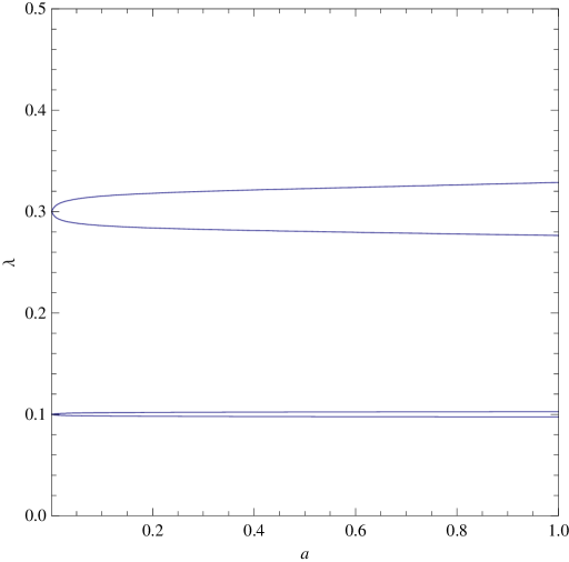
Figure 1: Plot of $\lambda$ as a function of scale factor $a$. $W$ has been choosen to be 0.05. The lower set is for $\lambda_{0}=0.1$ and the upper set is for $\lambda_{0}=0.3$. For each set the upper line is $V(\phi)=\phi^{2}$ and the lower line is for $V(\phi)=\phi^{-2}$.

Assuming that these conditions are satisfied, one can use (25) to show that $\lambda$ is approximately constant during the evolution of the scalar field for different potentials, i.e $\lambda=\lambda_{0}$ where $\lambda_{0}$ is some initial value corresponding to the inital scalar field value $\phi_{0}$. In figure 1, we have shown that this is indeed true. For a particular value of $W$, $W=0.05$, we have shown that the variation of $\lambda$ during the entire evolution is very small from its initial value $\lambda_{0}$ for two completely different potentials e.g $V(\phi)=\phi^{2}$ and $V(\phi)={\phi^{-2}}$: for $\lambda_{0}=0.1$, $\lambda$ is practically constant, while for $\lambda_{0}=0.3$, the variation is ${\Delta\lambda\over{\lambda}}\leq 2.5\%$ from $a={10^{-3}}$ till today.

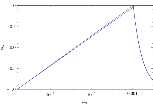
Figure 2: Plot of $\omega_{\phi}$ vs. $\Omega_{\phi}$ for $W=0.05$ and $\lambda_{0}=0.1$. Different lines are for $V(\phi)={\phi^{2}}$, $V(\phi)={\phi^{-2}}$ and our analytical expression (28).They are all practically indistinguishable.

So, we replace $\lambda$ by $\lambda_{0}$ in equation (II) and retain terms only to the lowest order in $\gamma$. Also we retain terms upto lowest order of $W$. Remember that $W$ is inversely related with the BD parameter $\omega$ which has to be large, resulting smaller value for $W$. This also ensures that the departure from the GR result is minimal. Using this, we obtain following equation:

$$\frac{d\gamma}{d{\Omega}_{\phi}} = \frac{-2\gamma}{\Omega_{\phi}(1-\Omega_{\phi})}+\frac{2}{\sqrt{3}}\frac{\lambda_{0}\sqrt{\gamma}}{\sqrt{\Omega_{\phi}}(1-\Omega_{\phi})}$$ (27)

$$+ \frac{2\sqrt{2}}{3}\frac{W\sqrt{\gamma}}{\Omega_{\phi}^{3/2}}$$

With $W=0$, one can get back to the solution $\gamma(\Omega_{\phi})$ as obtained earlier by Scherrer and Sen scherrer ; anjan . With $W$ one can also integrate the above equation to get the corresponding $\gamma(\Omega_{\phi})$. In order to do that one need to have some boundary condition to determine the integration constant arising due to integration of (27). The ideal condition should be $\gamma=0$ for $\Omega_{\phi}=0$. That is to say we start at very early time, when the dark energy contribution is zero and put the scalar field at the flat part of the potential. We can not take the limit $\Omega_{\phi}=0$ initially as term involving $W$ in the expression for $\gamma$ after integration, blows up. Instead we assume that for some very small initial value of $\Omega_{\phi}$, say $\Omega_{i}$, $\gamma_{i}=0$. We should stress that $\Omega_{i}$ can be very very small but not exactly zero. With this initial condition, one can get the equation of state:

$$1+\omega_{\phi}=[\frac{\lambda_{0}}{\sqrt{3\Omega_{\phi}}} - \left(\frac{1}{\Omega_{\phi}}-1\right)[(\frac{\lambda_{0}}{2\sqrt{3}}-\frac{\sqrt{2}W}{3})$$ (28)

$$\times \log\left(\frac{1+\sqrt{\Omega_{\phi}}}{1-\sqrt{\Omega_{\phi}}}\right)-\alpha]]^{2},$$

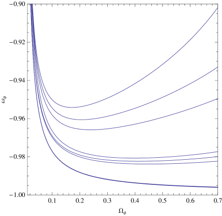
Figure 3: Plot of $\omega_{\phi}$ vs. $\Omega_{\phi}$ for $W=0.05$. The three sets are for $\lambda_{0}=0.1,0.2,0.3$ from bottom to top. For each set, top line is for $V(\phi)={\phi^{2}}$, the middle line is our analytical expression (28), and the bottom line is for $V(\phi)={\phi^{-2}}$.

where $\alpha=-\frac{\lambda_{0}}{\sqrt{3}}\frac{\sqrt{\Omega_{i}}\Omega_{i}}{1-\Omega_{i}}-\frac{2\sqrt{2}W}{3}\sqrt{\Omega_{i}}$. This is the main result we obtain in this study. This gives an analytical expression for the equation of state parameter for the dark energy as a function of its density parameter for a nonominimally coupled scalar field model (which is essentially a coupled quintessence model in Einstein frame). This generalizes the previous result obtained by Scherrer and Sen scherrer ; anjan for a corresponding minimally coupled scalar field model. The expression has an extra parameter $W$ which is related to the nonminimal coupling (or in other words related with the energy transfer between the matter and the dark energy in Einstein frame). The parameters $\lambda_{0}$ and $\Omega_{i}$ can be related with the present day value of the equation of state parameter $\omega_{\phi 0}$ of the scalar field and the corresponding value of its density parameter $\Omega_{\phi 0}$. Hence effectively the model has three parameters $W$, $\omega_{\phi 0}$ and $\Omega_{\phi 0}$.

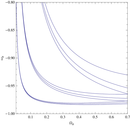
Figure 4: Plot of $\omega_{\phi}$ vs. $\Omega_{\phi}$ for $\lambda_{0}=0.3$.The three sets are for $W=0.05,0.1,0.2$ from bottom to top. For each set, top line is for $V(\phi)={\phi^{2}}$, the middle line is our analytical expression (28), and the bottom line is for $V(\phi)={\phi^{-2}}$.

Next we want to show that our analytical expression (28) for the equation of state parameter $\omega_{\phi}$ indeed represents the true behaviour for $\omega_{\phi}$ for variety of potentials $V(\phi)$ subject to the condition that all of them have a very flat part over which the scalar field rolls, i.e, $\lambda_{0}$ is small. One peculiar feature of the nonminimal coupling (or coupled quintessence) is that even though we start with a scalar field which is initially confined to the flat part of the potential leading to $\omega_{\phi i}=-1$, it starts increasing to a higher positive value initially before coming back to a negative value near $-1$. And this is not only for our approximate analytical expressions for $\omega_{\phi}$ given in (28), it is also true when we solve numerically the exact equations (23), (24), and (25). And this is solely due to the interaction between the matter and dark energy. This interaction term is related with matter energy density (see equation (13)) and as initially it is large, the interaction is also very large. This actually violates our assumption of $\gamma<<1$ initially. But we should emphasis that this does not create any problem for the viable cosmology as this peculiar behaviour happens only when $\Omega_{\phi}$ has negligible contribution to the total energy density of the universe, and does not contribute in any way to the cosmological evolution. Once $\Omega_{\phi}$, starts contributing substantially to the total energy density, the equation of state $\omega_{\phi}$ reaches value close to cosmological constant which is what we expect. In Figure 2, we have shown the behaviour of $\omega_{\phi}$ as a function of $\Omega_{\phi}$ for negligibly small values of $\Omega_{\phi}$. We have shown the behaviours for analytical expression (28) as well as the result obtained by numerically solving (23)-(25) for potentials $V(\phi)={\phi^{2}}$ and $V(\phi)={\phi^{-2}}$. The plots are shown for $W=0.05$ and $\lambda_{0}=0.1$ ($\Omega_{i}$ has been choosen so as to have $\Omega_{\phi}$ at present to be equal to 0.7). One can see the different behaviours are indistinguishable from each other, showing, (i) with small $\lambda_{0}$ different potentials have similar evolutions and (ii) our analytical expression (28) represents correctly the exact behaviour for small $\lambda_{0}$.

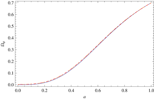
Figure 5: Plot of $\omega_{\phi}$ vs. scale factor $a(t)$ for $\lambda_{0}=0.3$, $\Omega_{\phi 0}=0.7$. The three sets are for $W=0.1$. The solid line is for (29), the dashed line for $V(\phi)={\phi^{2}}$, and the dotdashed line is for $V(\phi)={\phi^{-2}}$. As one can see all three lines are indistinguishable.

In figure 3 and figure 4, we show the same behaviour $\omega_{\phi}(\Omega_{\phi})$ for larger values of $\Omega_{\phi}$. We have plotted $\omega_{\phi}$ as a function of $\Omega_{\phi}$ for our analytical result (28) as well as by solving numerically the exact equations (23) - (25) for different potentials, using different values of $W$ and $\lambda_{0}$. In each case, $\Omega_{i}$ has been chosen in order to have $\Omega_{\phi}$ at present to be equal to 0.7. The figures show that for small $\lambda_{0}$ our analytical expressions nicely represent the exact behaviours for completely different potentials.

Next we have to find the expression for $\Omega_{\phi}(a)$, in order to express $\omega_{\phi}$ as a function of the scale factor $a$. This is essential for confronting the model with any observational result. In this regard, we can use (23) to solve $\Omega_{\phi}(a)$ to use it subsquently to determine $\omega_{\phi}(a)$. Assuming both $\gamma$ and $W$ to be small, we can neglect the terms involving those in (23), to get an approximate solution for $\Omega_{\phi}$:

$$\Omega_{\phi}=[1+(\frac{1}{\Omega_{\phi 0}}-1){a^{-3}}]^{-1}$$ (29)

where $\Omega_{\phi 0}$ is the the present day value of $\Omega_{\phi}$ and we normalize the present scale factor to $1$. This is same as what we get for a $\Lambda$CDM model which is not unexpected as we are considering scalar fields which have equation of state very close to $-1$. To show that this form for $\Omega_{\phi}$ very closely resembles with what one gets by exactly solving the (23)-(25) for small $\lambda_{0}$, we show the plots in figure 5. Here we plot our analytical expression (29) for $\Omega_{\phi}$ together with the result one obtains for $\Omega_{\phi}$ by solving numerically the exact equations (23)-(25). We have fixed $W=0.1$ and $\lambda_{0}=0.3$ for this purpose and assume $\Omega_{\phi 0}=0.7$. One can see that all three lines are just indistinguishable, confirming the fact that our analytical approximation (29) for $\Omega_{\phi}$ is indeed robust. It also shows the contribution of the scalar field to the total energy density of the universe is negligibly small till $a\sim 0.2$ and any peculiar behaviour of the equation of state $\omega_{\phi}$ before this era does not matter in any way.

So (28) together with the (29) for $\Omega_{\phi}(a)$ represents an analytical behaviour for the equation of state of a non-minimally coupled scalar field with BD type coupling. This behaviour is only valid when the scalar field rolls over a very flat part of the potential so that equations (2) and (3) are satisfied, irrespective of the form of the potential. This is main result of this study and its generalizes the similar result obtained earlier by Scherrer and Sen scherrer ; anjan for minimally coupled scalar fields.

III Observational Constraints

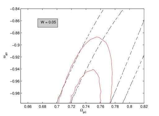
Figure 6: $1\sigma$ and $2\sigma$ confidence contours in $\omega_{\phi 0}-\Omega_{\phi 0}$ plane. The dashed lines are for SnIa data only and the solid lines are for SnIa+Bao data (explained in the text). This is for $W=0.05$.

Next we compare our result for $\omega_{\phi}(a)$ to the SnIa and Baryon Acoustic Oscillations data. The confidence contours are constructed using 60 Essence supernovae, 57 SNLS (Supernova Legacy Survey) and 45 nearby supernoave, and the data released by 30 SnIa detected by HST and classified as Gold sample by Riess et al riess . The combined data set can be found in Ref. davis . We also add the result obtained by Sloan Digital Sky Survey regarding the Baryon Acoustic Oscillation (BAO) Peak, giving a distance scale at $z_{bao}=0.35$. In Figure 6,7 and 8 we have shown the confidence contours for $W=0.05$, $W=0.1$ and $W=0.2$.

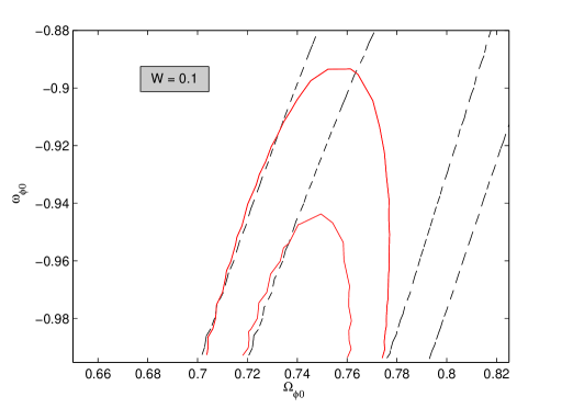
Figure 7: $1\sigma$ and $2\sigma$ confidence contours in $\omega_{\phi 0}-\Omega_{\phi 0}$ plane. The dashed lines are for SnIa data only and the solid lines are for SnIa+Bao data (explained in the text). This is for $W=0.1$.

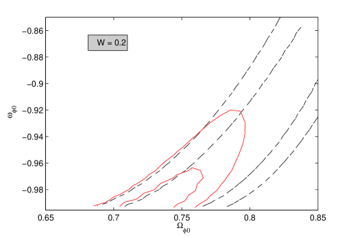
Figure 8: $1\sigma$ and $2\sigma$ confidence contours in $\omega_{\phi 0}-\Omega_{\phi 0}$ plane. The dashed lines are for SnIa data only and the solid lines are for SnIa+Bao data (explained in the text). This is for $W=0.2$.

Our result shows that cosmological constant is obviously very much consistent with the observational result. Also, unless one obtains a stringent bound on $\Omega_{m0}$ from structure formation data e.g the shape parameter for the matter power spectrum, which will result a corresponding bound on $\Omega_{\phi 0}$, one can not put a strong constraint on $\omega_{\phi 0}$, although BAO data seems to provide a strong upper bound for $\omega_{\phi}$ which is around $\omega_{\phi 0}\leq-0.92$.

IV Conclusion

We have studied dark energy models with scalar fields which are non-minimally coupled to gravity. We assume the form of the coupling is of BD type. We write the system of equations in conformally transformed Einstein frame where the scalar field becomes coupled with the matter sector although minimally coupled with the gravity sector. Our model is exactly similar to the coupled quintessence models considered previously by several authors coupled . To study such coupled quintessence models, we have assumed that the coupling parameter $W$ between the matter and dark energy (which is related with BD parameter $\omega$ in Jordan frame) is small. This ensures that our model does not deviate much from the standard Einstein gravity.

With a such a system, we consider potentials for the scalar fields which satisfy the slow-roll conditions (2), (3). In such a scenario, we show that all of them converge to a universal behaviour given by (28) and (29). This work generalizes the previous result by Scherrer and Sen obtained for minimally coupled scalar fields, to the non-minimally coupled case which can also be described as a coupled quintessence model in Einstein frame.

In this model, one has to fine tune the initial conditions in order to get desired value for the equation of state or density parameters at present which is in contrary to the so-called tracker model. But here the subsequent evolution of the universe is insensitive to the form of the potential as long as the slow-roll conditions (2), (3) are met. This is in contrast to the tracker models where one has to really fine tune the shape of the potential in order to achieve the tracker behaviour.

We have also tested our model with the observational data from SnIa and BAO peak. Although to get strong bound on the equation of state, one needs to have strong independent observational constraint on $\Omega_{\phi 0}$, still inclusion of BAO data put a strong upper bound on $\omega_{\phi 0}$ irrespective of the value of $W$, the coupling parameter.

V Acknowledgement :

AAS acknowledges the financial support provided by the University Grants Commission, Govt. Of India, through the major research project grant (Grant No: 33-28/2007(SR)). Part of the work has been done at IUCAA, Pune (India) during the visit of AAS under associateship program. SD would like to thank Relativity and Cosmology Research Centre, Jadavpur University, Kolkata where part of this work has been done.

References

- (1) A. G. Riess et al., Astron. J. 116, 1009 (1998); S. Perlmutter et al., Bull. Am. Astron. Soc. 29, 1351 (1997); S. Perlmutter et al., Astrophys. J. 517, 565 (1999); J. L. Tonry et al., Astrophys. J. 594, 1 (2003).
- (2) A. Melchiorri et al., Astrophys. J. Lett. 536, L63 (2000); A. E. Lange et al., Phys. Rev. D 63, 042001 (2001); A. H. Jaffe et al., Phys. Rev. Lett. 86, 3475 (2001); C. B. Netterfield et al., Astrophys. J. 571, 604 (2002); N. W. Halverson et al., Astrophys. J. 568, 38 (2002).
- (3) S. Bridle, O. Lahab, J. P. Ostriker and P. J. Steinhardt, Science 299, 1532 (2003); C. Bennett et al., Astrophys. J. Suppl. Ser. 148, 1 (2003); G. Hinshaw et al., Astrophys. J. Suppl. Ser. 148, 135 (2003); A. Kogut et al., Astrophys. J. Suppl. Ser. 148, 161 (2003); D. N. Spergel et al., Astrophys. J. Suppl. Ser. 148, 175 (2003).
- (4) E. J. Copeland, M. Sami and S. Tsujikawa, Int. J. Mod. Phys. D 15, 1753 (2006).
- (5) W. M. Wood-Vasey et al., Astrophys. J. 666, 694 (2007).
- (6) T. M. Davis et al., Astrophys. J. 666, 716 (2007).
- (7) R. J. Scherrer and A. A. Sen, Phys. Rev. D 77, 083515 (2008).
- (8) R. J. Scherrer and A. A. Sen, Phys. Rev. D, 78, 067303 (2008).
- (9) P. Jordan, Z. Phys.157, 112 (1959).
- (10) C. Brans and R.H. Dicke, Phys. Rev. D 124, 925 (1961).
- (11) T. Damour and G. Esposito-Farese, Class. Quant. Grav. 9, 2093 (1992); T. Damour and G. Esposito-Farese, Phys. Rev. D 53, 5541 (1996); T. Damour and G. Esposito-Farese, Phys. Rev. D 54, 1474 (1996); C. M. Will, Phys. Rev. D 50, 6058 (1994); T. Damour and G. Esposito-Farese, Phys. Rev. D 58, 042001 (1998); T.Damour and K. Nordtvedt, Phys. Rev. Lett. 70, 2217 (1993).
- (12) N.Banerjee and S. Sen, Phys. Rev. D 56, 1334 (1997).
- (13) A. Guth, Phys. Rev. Lett. 49, 1110 (1982).
- (14) D. La and P. J. Steinhardt, Phys. Rev. Lett., 62, 376 (1989).
- (15) M. Gasperini and G. Veneziano, Astropart. Phys. 1, 317 (1993).
- (16) N. Banerjee and D. Pavon, Class. Quant. Grav., 18, 593 (2001); A. A. Sen and S. Sen, Mod. Phys. Lett. A 16, 1303 (2001); S. Sen and A. A. Sen, Phys. Rev. D 63, 124006 (2001); J. P. Uzan, Phys. Rev. D 59, 123510, (1999); T. Chiba, Phys. Rev. D 60, 083508 (1999); F. Perrotta, C. Baccigalupi and S. Matarrese, astro-ph/9906066; E. Elizalde, S. Nojiri and S. Odintsov, Phys. Rev. D 70, 043539 (2004); V. K. Onemli and R. P. Woodard, Class. Quantum Grav. 19, 4607 (2002); V. K. Onemli and R. P. Woodard, Phys. Rev. D 70, 107301 (2004); T. Brunier, V. K. Onemli and R. P. Woodard, Class. Quant. Grav. 22, 59 (2005); E. Elizalde et al., Phys. Rev. D 77, 106005 (2008); N. Banerjee and S. Das, Mod. Phys. Lett. A 21, 2663 (2006).
- (17) A. R. Liddle and R. J. Scherrer, Phys. Rev. D 59, 023509 (1998).
- (18) V. Faraoni, gr-qc/0002091.
- (19) N. Bertolo and M. Piertroni, hep-th/9908521.
- (20) O. Bertolami and P. J. Martins, Phys. Rev. D 61, 064007 (2000).
- (21) R. de Ritis, A. A. Marino, C. Rubano and P. Scudellaro, Phys. Rev. D. 62, 043506 (2000).
- (22) S. Sen and T. R. Seshadri, gr-qc/0007079.
- (23) T.D. Saini, S. Raychaudhury, V. Sahni and A. A. Starobinsky, Phys. Rev. Lett. 85, 1162 (2000).
- (24) B. Boisseau, G. Esposito-Farese, D. Ploarski and A. A. Starobinski, Phys. Rev. Lett. 85, 2236 (2000).
- (25) S. Das and N. Banerjee, Gen. Relativ. Gravit. 38, 785 (2006); S Das and N. Banerjee, Phys. Rev. D 78, 043512 (2008).
- (26) L. Amendola, Phys. Rev. D. 62, 043511 (2000); G. R. Farrar and P. J. E. Peebles, Astrophys. J. 604, 1 (2004); G. R. Farrar and R. A. Rosen, Phys. Rev. Lett. 98, 17, (2007); C. Wetterirch. Astron. Astrophys., 301, 321 (1995).
- (27) A. W. Brookfield et al., Phys. Rev. D. 77, 043006 (2008); G. Mangano et al., Mod. Phys. Lett. A 18, 831, (2003); M. Quartin et al, JCAP, 0805, 007 (2008).
- (28) O. Bertolami et al., Phys. Lett. B 654, 165 (2007); S. Lee et al., Phys. Rev. D 73, 083516 (2006); Z-K. Guo et al., Phys. Rev. D. 76, 023508, (2007); R. Mainini and S. Bonometto, JCAP, 0706, 020 (2007); B. Wang, Nucl. Phys., B778, 69 (2007).
- (29) D. J. Holden and D. Wands, Phys. Rev. D 61, 043506 (2000); [gr-qc/9908026].
- (30) S. Dodelson, M. Kaplinghat and E. Stewart, Phys. Rev. Lett. 85, 5276 (2000).
- (31) A. G. Riess et al., Astrophys. J. 607, 665 (2004); A. G. Riess et al., Astrophys. J. 659, 98 (2007).