Using constraint programing to resolve the multi-source / multi-site data movement paradigm on the Grid

Abstract:

In order to achieve both fast and coordinated data transfer to collaborative sites as well as to create a distribution of data over multiple sites, efficient data movement is one of the most essential aspects in distributed environment. With such capabilities at hand, truly distributed task scheduling with minimal latencies would be reachable by internationally distributed collaborations (such as ones in HENP) seeking for scavenging or maximizing on geographically spread computational resources. But it is often not all clear (a) how to move data when available from multiple sources or (b) how to move data to multiple compute resources to achieve an optimal usage of available resources. Constraint programming (CP) is a technique from artificial intelligence and operations research allowing to find solutions in a multi-dimensional space of variables. We present a method of creating a CP model consisting of sites, links and their attributes such as bandwidth for grid network data transfer also considering user tasks as part of the objective function for an optimal solution. We will explore and explain trade-off between schedule generation time and divergence from the optimal solution and show how to improve and render viable the solution’s finding time by using search tree time limit, approximations, restrictions such as symmetry breaking or grouping similar tasks together, or generating sequence of optimal schedules by splitting the input problem. Results of data transfer simulation for each case will also include a well known Peer-2-Peer model, and time taken to generate a schedule as well as time needed for a schedule execution will be compared to a CP optimal solution. We will additionally present a possible implementation aimed to bring a distributed datasets (multiple sources) to a given site in a minimal time.

1 Introduction

1.1 Problem area

Computationally challenging experiments such as the one from the High Energy and Nuclear Physics community (HENP) have developed a distributed computing approach (a.k.a. Grid computing model) to face the massive needs of their Peta-scale experiments. The era of data intensive computing has surely opened a vast arena for computer scientists to resolve practical and exciting problems. One of such HENP experiments is the STAR (Solenoidal Tracker at Relativistic Heavy Ion Collider) experiment located at the Brookhaven National Laboratory (USA).

In addition to a typical Peta-scale challenge and large computational needs, this experiment, as a running experiment acquires a new set of valuable real data every year, introducing other dimension of safe data transfer to the problem. From the yearly data sets, the experiment may produce many physics ready derived data sets which differ in accuracy as the problem is better understood as time passes. Thus, demands for a large-scaled storage management and efficient scheme to distribute data grows as a function of time, while on the other hand, end-users may need to access data sets from previous years and consequently at any point in time. Coordination is needed to avoid random access destroying efficiency.

The user’s task is typically embarrassingly parallel; that is, a single program can run $N$ times on fraction of the whole data set split into $N$ sub-parts without any impact on science reliability, accuracy, or reproducibility. For a computer scientist, the issue then becomes how to split the embarrassingly parallel task into N jobs in the most efficient manner while knowing the data set is spread over the world and/or how to spread ’a’ dataset and best place the data for maximal efficiency and fastest processing of the task.

The purpose of this work is to design and develop an automated system that would efficiently use all available computational and storage resources. It will relieve end users of making decisions among possible ways of their task execution (which includes locating and transferring data to desired sites that appear optimal to user) while preserving fairness. Users’ knowledge of the whole system and data transfer tools will be reduced just to the communication with the future planner that will guarantee its decision to spread the task and data sets over chosen sites was, under current circumstances, the most efficient and optimal.

1.2 Milestones

Rather than trying to solve the problem directly from a task scheduling perspective within a grid environment, we split the problem into several stages. By isolating data transfer/placement and computational challenges from each other we get an opportunity to study the behavior of both sets of constraints separately.

Individual tasks depend on a datasets which size has to be considered as well, since the time required for its staging and transfers is also significant. Therefore, the first milestone is to design and develop the data transfer planner/scheduler. For a given dataset needed at some site, its aim is to create a plan with an objective to prepare files from the dataset at a given site within the shortest time. The next requirement is to define and achieve fair share transfers within a multiuser environment. This means that if one user asked for a huge amount of data at some site, then another user who asked just for one file shouldn’t wait until the first user’s plan is finished.

The next milestone generalizes data transfer planning between sites. The goal for this stage is not to transfer files to one particular site, but do the transfer to several destinations. More precisely, the planner’s goal is to achieve presence of each file (from user’s input task) at one out of all possible destinations, while still having the objective in mind, to minimize the finish time of the last file transfer the user waits for.

The second milestone is highly corellated with the final milestone - scheduling the data transfers together with particular tasks (jobs) on a grid. The subtask is not finished after a file is transfered at some destination site, but when the user’s job executed at the same site (and dependent on this file) is finished. Thus, the planner still has the freedom of choosing a destination site for each file, but it has to consider that each site has a specific characteristic of its computational performance. These attributes include, for example, the number of available CPUs at current site or the actual load, so it can be more effective to transfer some files over the slower link to the computationally high performance site (or vice versa). The final objective is to minimize the finish time of the last user’s job. In this article we focus on the first milestone.

2 Problem formalization

In the following part we will present a formal description of the problem and an approach based on Constraint Programming technique, used in artificial intelligence and operations research, where we search for assignment of given variables from their domains, in such a way that all constraints are satisfied and value of an objective function is optimal [3].

We will introduce the transfer network consisting of sites holding information which files are available at the site. For each file we will search for a path leading to the destination and time slots for each link on transfer path, when a particular file transfer should occur.

The network consists of a set of nodes $\mathbf{N}$ and a set of directed edges $\mathbf{E}$. The set $\mathbf{OUT}(n)$ consists of all edges leaving node $n$, the set $\mathbf{IN}(n)$ of all edges leading to node $n$. Input received from a user is a set of file names needed at a destination site $\mathbf{dest}$. We will refer to this set of file names as to demands, represented by $\mathbf{D}$. For every demand $d$ we have a set of sources ($\mathbf{orig}(d)$), sites where the file ($d$) is already available. We will use one decision variable for every demand and link of the network (edge in graph). The $\{0,1\}$ variable $X_{de}$ denotes whether demand $d$ is routed over edge $e$ of the network. The second variable $start_{de}$ denotes start time of transfer corresponding to the demand $d$ over edge $e$. More approaches can be found in [5].

$$\min_{X_{de},start_{de}}\max_{e\in\mathbf{E}}\underbrace{\left(start_{de}+\frac{size(d)}{speed(e)}\right)}_{end_{de}}\cdot X_{de}$$ (1)

$$\forall d\in\mathbf{D}:\sum_{e\in\cup\mathbf{OUT}(n|n\in\mathbf{orig}(d))}X_{de}=1,\,\sum_{e\in\cup\mathbf{IN}(n|n\in\mathbf{orig}(d))}X_{de}=0$$ (2)

$$\forall d\in\mathbf{D}:\sum_{e\in\mathbf{OUT}(dest(d))}X_{de}=0,\;\sum_{e\in\mathbf{IN}(dest(d))}X_{de}=1$$ (3)

$$\begin{split}&\forall d\in\mathbf{D},\forall n\notin\{orig(d)\cup dest(d)\}:\\ \sum_{e\in\mathbf{OUT}(n)}X_{de}\leq 1,&\;\sum_{e\in\mathbf{IN}(n)}X_{de}\leq 1,\;\sum_{e\in\mathbf{OUT}(n)}X_{de}=\sum_{e\in\mathbf{IN}(n)}X_{de}\end{split}$$ (4)

$$\forall e\in\mathbf{E},\forall d\in\mathbf{D}:X_{de}=1:\bigcap[start_{de},\underbrace{start_{de}+\frac{size(d)}{speed(e)}}_{end_{de}}]=\emptyset$$ (5)

$$\forall n\in{\mathbf{N}},\forall d\in\mathbf{D}:\sum_{e\in\mathbf{IN}(n)}\underbrace{\left(start_{de}+\frac{size(d)}{speed(e)}\right)}_{end_{de}}\cdot X_{de}\leq\sum_{e\in{\mathbf{OUT}}(n)}start_{de}\cdot X_{de}$$ (6)

$$\begin{array}[]{c}X_{de}\in\{0,1\}\\ start_{de}\in{\cal N^{+}}\end{array}$$

The path constraints (2, 3, 4) state that there is a single path for each demand (path starting right in one of origin sites, leading to the destination). Equation (5) ensures there is only one active file transfer over every edge in time. The last equation states that a transfer of the file at any site can start only if the file is already available at the site (Eq. 6)(i.e., a transfer of the file to this site has finished). The objective (Eq. 1) is to minimize the latest finish time of transfer over the whole files.

2.1 Constraint model

For implementation of the solver we use Choco , a Java based library for constraint satisfaction problems (CSP), constraint programming (CP). Among $70$ available constraints Choco provides also a set for scheduling and resource allocation, we require most. Closer illustration of several Choco uses can be found in [1], [2], and [6]. In addition, Java based platform allows us an easier scheduler integration with currently used tools in the STAR environment.

Constraints introduced in the previous section were used directly via appropriate Choco structures, except the equation 5, that ensures at most single file transfer in any time on any link. For this, we used the cumulative scheduling constraint and notation of tasks and resources. Tasks are represented by their duration, by ranges for starting and ending times, and by resource consumption respectively. They are allocated to the resource(s) in such a way that in any time resource capacity can not be exceeded.

In our case, each link acts as a separate resource with capacity $1$ (unary resource) and each file demand creates a single task on every resource, which duration depends on the current link speed (resource characteristic) and consumption of the resource corresponds to the value of variable $X$, i.e. no consumption if the transfer path for demand does not include current link (resource), or consumption 1 otherwise. In the Figure (1) is shown one possible schedule for transferring one file ($F$) with an origin at $Site_{1}$ and $Site_{2}$ to a destination $Dest$. Values of the $X$ variables define the path, while the resource profile for each link is on the right side.

Figure 1: Example of a schedule solution with file $F$ and its origin at $Site_{1}$ and $Site_{2}$.

The search strategy, following Choco notation, is split into two goals. First one is to find assignment for $X$ variables, i.e. paths for each transfer, while the second is to allocate time slot, assign $start$ variables, for each transfer at chosen links. For both goals the default ‘minimum domain‘ variable selection and ‘increasing value‘ value selection heuristic were used.

3 Direct connections

In order to closely analyze the problem, its scale, and behavior of used techniques, we started with several restrictions that simplify the case. We started to explore the network, where only direct connections for data movement are allowed. In other words, file can not be transferred from its origin to the destination by a path longer than one.

One can think that such a restriction shrinks the search space enormously, but closer look reveals that the number of possible combinations is still large:

Let’s suppose that we have a network of $5$ sites, all connected to the destination and $100$ files available at each site ($|orig(f)|=5$). The number of decision variables $X$ is therefore $500$ ($=|D|*|E|$). Even if an upper bound for all possible combinations ($2^{500}$) is reduced by a propagation to $5^{100}$ (solver has a freedom of 5 choices of an origin for each file), brute-force methods can run ’forever’.

With an intend to stay close to a reality, we fixed the number of sites to $5$, which approximately represents the number of sites currently available in the STAR experiment. For each link we introduced a slowdown factor that influences the transfer time needed to move the data over this link. Slowdown factor $1$ means that file of size $1$ unit can be transferred in $1$ unit of time, but with a slowdown factor $4$ only in $4$ units of time, etc.

Considering the second part of the input, the file demands, we studied the following cases: a) every file is available only at one particular site [distinct]; b) file is available at sites given by a probability function, that represents the reality [weighted]; c) file is available at all sites [shared]. For all cases we fixed the file size to a $1$ unit, i.e. all files have the same size.

3.1 Shared links

So far we have assumed that all links incoming or outgoing from any site have their own bandwidth (slowdown factor) that is not affected by other ones. Nevertheless, in reality this is not always feasible, since several links leading to a site usually share the same router and/or physical fiber which bandwidth (capacity) is less than the sum of their own values. Hence, simultaneously one can’t use all links at their maximum bandwidths. We express this constraint by adding an additional resource per each group of shared links. Capacity of the resource will be the bandwidth of a shared link or a router, while tasks correspond to the scheduled transfers using any link belonging to this group with consumptions equal to its slowdown factor.

3.2 Reducing a search time

We studied also several techniques for reducing the time spent during a search.

3.2.1 Symmetry breaking

One of the common techniques for reducing the search tree is detecting and breaking variable symmetries. This is usually done by adding variable symmetry breaking constraints that can be expressed easily and propagated efficiently using lexicographic ordering. One idea that can be applied in the studied case (direct connections and fixed file size) is following: if two files have the same origin sets, links selected for the first one and for the second one respectively must be ordered. The reason behind is that both files must be transferred to the destination and their size is equal, it is not necessary to check also ’swapped’ case, since the transfer time can not be shorter.

3.2.2 Decomposition and search limits

Another approach is based on the idea, where instead of searching for a global optimal solution that can be very computing time consuming, we try to find an optimal solution for smaller parts of the input, where sum of the time spent will be just a portion of time needed otherwise. This principle is even more suitable for our needs, since network link speeds vary in time, some sites can be down after the schedule is produced, generally, transferring all data files takes significant amount of time and during this time a lot of factors can be different to the ones the scheduler considered at the beginning. Thus the computed optimal schedule for the full input doesn’t have to be valid anymore.

One of the approximations is splitting the input files into chunks and producing an optimal schedule for each chunk separately, while propagating the results from the previous ones. More precisely, result of the scheduler for a given chunk of files is information of computed starting/ending times for each file at particular links. In other words, current solver receives times for each link, by which the link will be busy, thus further scheduling for current chunk cannot place file transfer in these time-slots. We achieve this by allocating a fake task, with fixed starting and ending times, that were propagated from previous schedules (Figure: 2).

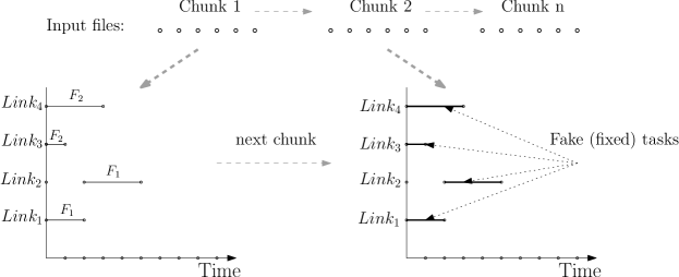
Figure 2: Allocating fake tasks according to the previous schedule.

Also limits can be imposed on the search algorithm to avoid spending too much time in the exploration. One of them is fixing the time limit on a search tree. When the execution time is equal to the time limit, the search stops whether an optimal solution is found or not. One of the algorithms we studied was based on this, with a time-limit linearly dependent on the number of files in a request.

4 Directed (simple) paths

Considering the model, no changes are necessary to perform in order to allow solver search for transfer paths longer than one. However, since data set transit takes some storage space, one must be sure that during file transfer from site A to C, using site B, there is enough space at intermediate site B.

4.1 Storage capacity

In order to respect storage restrictions we introduce the next attribute for each site, the available (free) space, or the storage capacity. All the time during the execution of a schedule, the storage capacity constraint for each site must be respected.

For each site we consider all possible ways (pairs of $inLink$ and $outLink$ how a file can be transferred trough it. Whether or not a pair is really used for the demand $d$ is expressed by $channelingVariable$, using which we define also consumption of the task (Figure: 3).

Figure 3: Storage resource and representation of the consumption of a free space at site during transferring a file through it.

If the pair is not used, the consumption is set to zero and storage resource is invariable to this task, otherwise the consumption is set to the file size.

5 Comparative studies

In this section we present the performance comparison of several methods of the CSP solver introduced in previous sections as well as of the Peer-2-Peer simulator. We will also show an effect of one constraint (storage based) for a simple paths case and an example of the optimal schedule produced by the solver.

5.1 Peer-2-Peer simulator

To provide a base comparison with the results of our CSP based solver we chose to implement a Peer-2-Peer (P2P) model as well. This model is well known and successfully used in similar fields like file sharing, telecommunication, or media streaming. We implemented a P2P simulator by creating the following work-flow: a) put an observer for each link leading to the destination; b) if an observer detects the link is free, it picks up the file at his site (link starting node), initiate the transfer, and waits until the transfer is done. We introduced a heuristic for picking up a file as typically done for P2P. Link observer picks up a file with a smallest cardinality in the sense of its $|origin|$, i.e. the file that is available at the smallest number of sites and if there are more files available with the same cardinality, it randomly picks any of them. After each transfer, the file record is removed from the list of possibilities over all sites. This process is typically resolved using distributed hash table (DHT) [4], however in our simulator only simple structures were used. Finally an algorithm finishes when all files reach the destination, thus no observer has any more work to do.

5.2 Results

In Figure 4, we show a comparison of times needed to produce the schedules and divergence of the results (makespan) to the optimal solution between several algorithms. We present results only for weighted case with direct connections and will only describe the qualitative features for the other cases. Weights (probabilities) that were used for sites considering file’s origins were $1.0,0.6,0.01,$ and $0.01$.

The X axes denote the number of files in a request while Y is the time (in units) needed to generate the schedule and percentage loss on optimal solution. We can see that time to find an optimal schedule without any additions grows exponentially and is usable only for a limited number of files, $50$ in the weighted case and $20$ in the shared case. This difference is induced by a higher number of possible configurations as long as any site can be selected as an origin. By introducing symmetry breaking, the solving time is improved, but still not usable for more than $200$ files. Using the time-limit on the other hand we are moving apart from an optimal solution with increasing files in request, which is even more visible in shared case. Thus setting the time-limit as a linear function to the number of files, while using a default search strategy based on minimal domains, is not sufficient.

In contrast, splitting the input into chunks is giving the best performance results both in the running time and also in the quality of the makespan. Even scheduling by chunk of size $1$, i.e. file by file, doesn’t produce worse result than using larger chunks due to previous conditions propagation. We note as well the efficacious performance of a simple P2P algorithm, but it is worth to mention that this model is usable only in a direct connection case, while our intent is to study more complex networks with much more restrictions.

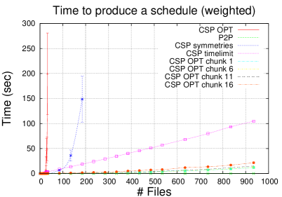
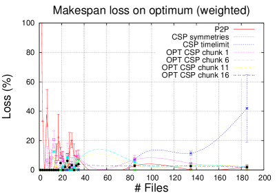
Figure 4: Approximation of the runtime (left) and makespan loss on optimal schedule (right) for weighted case.

To see the real effect of the storage constraint, in Gantt charts (Figure 5) are shown two schedules (without and with enabled constraint) for the same dataset, considering the funnel network displayed in the upper part of the figure with a limited available space at $Site_{3}$ only for one file size unit. This extreme example permits only a single transfer via site $Site_{3}$, that fills available space until a file is fully transfered to the destination $Site_{4}$. After that, the space at $Site_{3}$ is again released and another file can go trough.

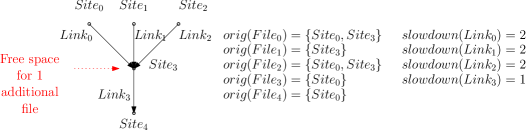
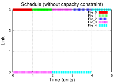
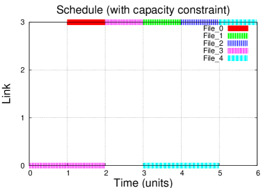
Figure 5: Gantt chart of a schedule without storage constraints (left) and a schedule with storage constraints (right) generated on the funnel network with limited storage capacity (up).

6 Conclusion

We presented an approach using a Constraint Programming model to tackle the efficient data transfers/placements and job allocations problem within a distributed environment. Usage of constraints and declarative type of programming offers straightforward way of representing many real life restrictions which is also less vulnarable to dragging bugs in an expanding code. On the other hand, since a search space is usually extensive, methods like symmetry breaking or approximations and understanding the scale of the problem are fundamental. We showed that using the scheduling of data transfers by sequence of smaller chunks gives results close to the optimal solution and provides very acceptable running time performance. We have implemented also several constraints for dealing with shared network links or limited storage capacities at sites and actual results indicate that it is worth to continue research with this technique.

References

- [1] David Benavides, Sergio Segura, Pablo Trinidad Martín-Arroyo, and Antonio Ruiz Cortés. Using java CSP solvers in the automated analyses of feature models. In Ralf Lämmel, João Saraiva, and Joost Visser, editors, GTTSE, volume 4143 of Lecture Notes in Computer Science, pages 399–408. Springer, 2006.
- [2] Alexander Lazovik, Marco Aiello, and Rosella Gennari. Choreographies: using constraints to satisfy service requests. In AICT/ICIW, page 150. IEEE Computer Society, 2006.
- [3] K. Marriott and P. Stuckey. Programming with Constraints. MIT Press, Cambridge, Massachusetts, 1998.
- [4] Naor and Wieder. A simple fault tolerant distributed hash table. In International Workshop on Peer-to-Peer Systems (IPTPS), LNCS, volume 2, 2003.
- [5] Helmut Simonis. Challenges for constraint programming in networking. In Mark Wallace, editor, CP, volume 3258 of Lecture Notes in Computer Science, pages 13–16. Springer, 2004.
- [6] Jules White, Douglas C. Schmidt, Krzysztof Czarnecki, Christoph Wienands, Gunther Lenz, Egon Wuchner, and Ludger Fiege. Automated model-based configuration of enterprise java applications. In EDOC, pages 301–312. IEEE Computer Society, 2007.