Time-Varying Networks: Recovering Temporally Rewiring Genetic Networks During the Life Cycle of
Drosophila melanogaster

Abstract

Due to the dynamic nature of biological systems, biological networks underlying temporal process such as the development of Drosophila melanogaster can exhibit significant topological changes to facilitate dynamic regulatory functions. Thus it is essential to develop methodologies that capture the temporal evolution of networks, which make it possible to study the driving forces underlying dynamic rewiring of gene regulation circuity, and to predict future network structures. Using a new machine learning method called Tesla, which builds on a novel temporal logistic regression technique, we report the first successful genome-wide reverse-engineering of the latent sequence of temporally rewiring gene networks over more than 4000 genes during the life cycle of Drosophila melanogaster, given longitudinal gene expression measurements and even when a single snapshot of such measurement resulted from each (time-specific) network is available. Our methods offer the first glimpse of time-specific snapshots and temporal evolution patterns of gene networks in a living organism during its full developmental course. The recovered networks with this unprecedented resolution chart the onset and duration of many gene interactions which are missed by typical static network analysis, and are suggestive of a wide array of other temporal behaviors of the gene network over time not noticed before.

Introduction

A major challenge in systems biology is to understand and model, quantitatively, the topological, functional, and dynamical properties of cellular networks, such as transcriptional regulatory circuitry and signal transaction pathways, that control the behaviors of the cell.

Empirical studies showed that many biological networks bear remarkable similarities to various other networks in nature, such as social networks, in terms of global topological characteristics such as the scale-free and small-world properties, albeit with different characteristic coefficients (Barabasi & Albert, 1999). Furthermore, it was observed that the average clustering factor of real biological networks is significantly larger than that of a random network of equivalent size and degree distribution (Barabasi & Oltvai, 2004); and biological networks are characterized by their intrinsic modularities (Vászquez et al., 2004), which reflect presence of physically and/or functionally linked molecules that work synergistically to achieve a relatively autonomous functionality. These studies have led to numerous advances towards uncovering the organizational principles and functional properties of biological networks, and even identification of new regulatory events (Basso et al., 2005); however, most of such results are based on analyses of static networks, that is, networks with invariant topology over a given set of molecules, such as a protein-protein interaction (PPI) network over all proteins of an organism regardless of the conditions under which individual interactions may take place, or a single gene network inferred from microarray data even though the samples may be collected over a time course or multiple conditions.

Over the course of a cellular process, such as a cell cycle or an immune response, there may exist multiple underlying ”themes” that determine the functionalities of each molecule and their relationships to each other, and such themes are dynamical and stochastic. As a result, the molecular networks at each time point are context-dependent and can undergo systematic rewiring, rather than being invariant over time, as assumed in most current biological network studies. Indeed, in a seminal study by Luscombe & et al. (2004), it was shown that the ”active regulatory paths” in a gene expression correlation network of Saccharomyces cerevisiae exhibit dramatic topological changes and hub transience during a temporal cellular process, or in response to diverse stimuli. However, the exact mechanisms underlying this phenomena remain poorly understood.

What prevents us from an in-depth investigation of the mechanisms that drive the temporal rewiring of biological networks during various cellular and physiological processes? A key technical hurdle we face is the unavailability of serial snapshots of the rewiring network during a biological process. Under a realistic dynamic biological system, usually it is technologically impossible to experimentally determine time-specific network topologies for a series of time points based on techniques such as two-hybrid or ChIP-chip systems; resorting to computational inference methods such as structural learning algorithms for Bayesian networks is also difficult because we can only obtain a single snapshot of the gene expressions at each time point – how can one derive a network structure specific to a point of time based on only one measurement of node-states at that time? If we follow the naive assumption that each snapshot is from a different network, this task would be statistically impossible because our estimator (from only one sample) would suffer from extremely high variance. Extant methods would instead pool samples from all time points together and infer a single ”average” network (Friedman et al., 2000; Ong, 2002; Basso et al., 2005), which means they choose to ignore network rewiring and simply assume that the network snapshots are independently and identically distributed. Or one could perhaps divide the time series into overlapping sliding windows and infer static networks for each window separately. These approach, however, only utilizes a limited number of samples in each window and ignores the smoothly evolving nature of the networks. Therefore, the resulting networks are limited in term of their temporal resolution and statistical power. To our knowledge, no method is currently available for genome-wide reverse engineering of time-varying networks underlying biological processes with temporal resolution up to every single time point where gene expressions are measured.

Here, we present the first successful reverse engineering of a series of 23 time-varying networks of Drosophila melanogaster over its entire developmental course, and a detailed topological analysis of the temporal evolution patterns in this series of networks. Our study is based on a new machine learning algorithm called TEmporally Smoothed $L_{1}$-regularized LOgistic Regression, or Tesla (stemmed from TESLLOR, the acronym of our algorithm). Tesla is based on a key assumption that temporally adjacent networks are likely not to be dramatically different from each other in topology, and therefore are more likely to share common edges than temporally distal networks. Building on the powerful and highly scalable iterative $L_{1}$-regularized logistic regression algorithm for estimating single sparse networks (Wainwright et al., 2006), we develop a novel regression regularization scheme that connects multiple time-specific network inference functions via a first-order edge smoothness function that encourages edge retention in networks immediately across time points. An important property of this novel idea is that it fully integrates all available samples of the entire time series in a single inference procedure that recovers the wiring patterns between genes over a time series of arbitrary resolution — from a network for every single time point, to one network for every $K$ time points where $K$ is very small. Besides, our method can also benefit from the smoothly evolving nature of the underlying networks and the prior knowledge on gene ontology groups. These additional pieces of information increase the chance to recover biologically plausible networks while at the same time reduce the computational complexity of the inference algorithms. Importantly, Tesla can be casted as a convex optimization problem for which a globally optimal solution exists and can be efficiently computed for networks with thousands of nodes.

To our knowledge, Tesla represents the first successful attempt on genome-wide reverse engineering of time-varying networks underlying biological processes with arbitrary temporal resolution. Earlier algorithmic approaches, such as the structure learning algorithms for dynamic Bayesian network (Ong, 2002), learns a time-homogeneous dynamic system with fixed node dependencies, which is entirely different from our goal, which aims at snapshots of rewiring network. The Trace-back algorithm (Luscombe & et al., 2004) that enables the revelation of network changes over time in yeast is based on tracing active paths or subnetwork in static summary network estimated a priori from all samples from a time series, which is significantly different from our method, because edges that are transient over a short period of time may be missed by the summary network in the first place. The DREM program (Ernst et al., 2007) that reconstructs dynamic regulatory maps tracks bifurcation points of a regulatory cascade according to the ChIP-chip data over short time course, which is also different from our method, because Tesla aims at recover the entire time-varying networks, not only the interactions due to protein-DNA binding, from long time series with arbitrary temporal resolution.

A recent genome-wide microarray profiling of the life cycle of Drosophila melanogaster revealed the evolving nature of the gene expression patterns during the time course of its development (Arbeitman et al., 2002). In this study, 4028 genes were examined at 66 distinct time points spanning the embryonic, larval, pupal and adulthood period of the organism. It was found that most genes ($86\%$) were differentially expressed over time, and the time courses of many genes followed a wave structure with one to three peaks. Furthermore, clustering genes according their expression profiles helped identify functional coherent groups specific to tissue and organ development. Using Tesla, we successfully reverse-engineered a sequence of 23 epoch-specific networks from this data set. Detailed analysis of these networks reveals a rich set of information and findings regarding how crucial network statistics change over time, the dynamic behavior of key genes at the hubs of the networks, how genes forms dynamic clusters and how their inter-connectivity rewires overtime, and improved prediction of the activation patterns of already known gene interactions and link them to functional behaviors and developmental stages.

Results and Discussion

Time-Varying Gene Networks in Drosophila melanogaster

Tesla can reconstruct time-varying dynamic gene networks at a temporal resolution from one network per every time point to one network per epoch of arbitrary number of contiguous time points. From the 64-step long Drosophila melanogaster life cycle microarray time course, we reconstructed 23 dynamic gene networks, one per 3 time points, spanning the embryonic (time point 1–11), larval (time point 12–14), pupal (time point 15–20) and adulthood stage (time point 21–23) during the life cycle of Drosophila melanogaster (Fig. 1) . The dynamic networks appear to rewire over time in response to the developmental requirement of the organism. For instance, in middle of embryonic stage (time point 4), most genes selectively interact with other genes which results in a sparse network consisting mainly of paths. In contrast, at late adulthood stage (time point 23), genes are more active and each gene interacts with many other genes which leads to visible clusters of gene interactions. The global patterns of the evolution of the gene interactions in this network series are summarized in Fig 2. The network statistics include a summary of the degree distribution, network size in term of the number of edges, and the clustering coefficient of the networks, which are computed for each snapshot of the temporally rewiring networks. The degree distribution provides information on the average number and the extent that one gene interacts with other genes; the network size characterizes the total number of active gene interactions in each time point; and the clustering coefficient quantifies the degree of coherence inside potential functional modules. The change of these three indices reflects the temporally rewiring nature of the underlying gene networks.

All three indices display a wave pattern over time with these indices peaking at the start of the embryonic stage and near the end of adulthood stage. However, between these two stages, the evolutions of these indices can be different. More specifically, the degree distribution follows a similar path of evolution to that of the network size: there are three large network changes in the middle of embryonic stage (near time point 5), at the beginning of the larval stage (time point 11) and at the beginning of the adulthood stage (time point 20). In contrast, clustering coefficients evolve in a different pattern: in the middle of the life cycle there is only one peak which occurs near the end of the embryonic stage. This asynchronous evolution of the clustering coefficient from the degree distribution and network size suggests that increased gene activity is not necessarily related to functional coherence inside gene modules.

To provide a summary of the 23-epoch dynamic networks, gene interactions recovered at different time points are combined into a single network (Fig. 3(a)). The resulting summary network consists of 4509 distinctive interactions. Overall the summary network reveals a center of two giant clusters of tightly interacting genes, with several small loose clusters remotely connected to the center. The two giant clusters are each built around genes with high degree centrality. These two clusters and other small clusters are integrated as a single network via a set of genes with high betweenness centrality.

The top giant cluster is centered around two high degree nodes, protein coding gene eIF4AIII and CG9746. Both genes are related to molecular functions such as ATP binding. The selective interaction of these genes with other molecules modulates the biological functions of these molecules. In the bottom giant cluster, high degree nodes are more abundant compared to the top cluster. These high degree nodes usually have more than one functions. For instance, gene dsf and dsx are involved in DNA binding and modulate their transcription, which in turn regulates the sex related biological processes. Gene noc, CG14438, mkg-p are involved in both ion binding and intracellular component, while gene zfh1 and shn play important roles in the developmental process of the organism.

The connections between the clusters are very often channeled through a set of genes with high betweenness centrality. Note these genes do not necessarily have a high degree. They are important because they provide the relays for many biological pathways. For instance, gene fab1 is involved in various molecular functions such as ATP, protein and ion binding, while at the same time it is also involved in biological processes such as intracellular signaling cascade. Gene dlg1 participate in various functions such as protein binding, cell polarity determination and cellular component. Another gene tko participates in functions related to ribosome from both molecular, biological and cellular component point of views.

For comparison, a single static network of comparable size ($\sim$4500 gene interactions) is inferred by treating all measurements as independent and identically distributed samples (Fig 3(e)). The static network shares some common features with the summary graph of the dynamic networks. For instance, both networks reveal two giant clusters of interacting genes. However, the static network provides no temporal information on the onset and duration of each gene interaction. Furthermore, the static network and the summary graph of the dynamic networks follow very different degree distributions. The degree distribution of the summary graph of the dynamic networks has a much heavier tail than that of the static network (Fig 3(f)). In other words, the distribution for the dynamic networks resembles more to a scale free network while that for the static network resembles more to a random graph.

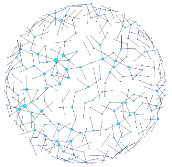
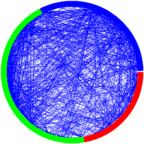
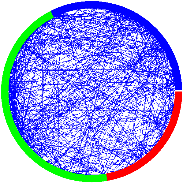
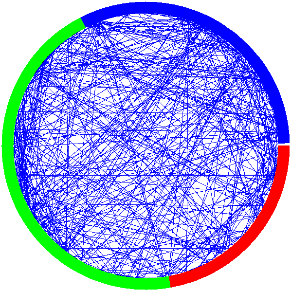
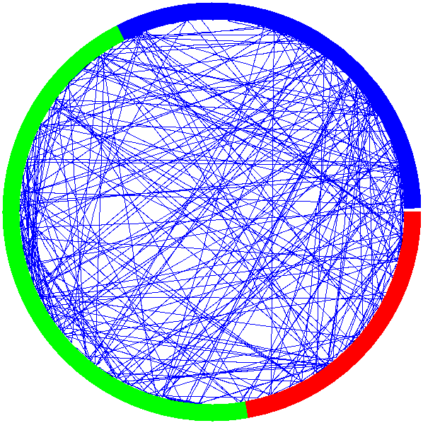
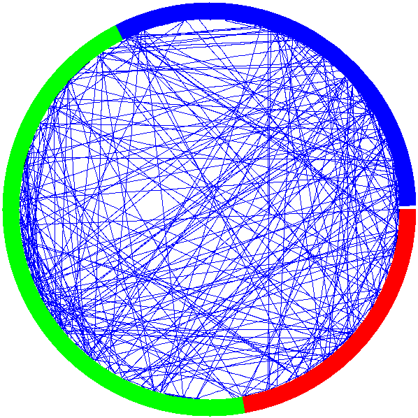
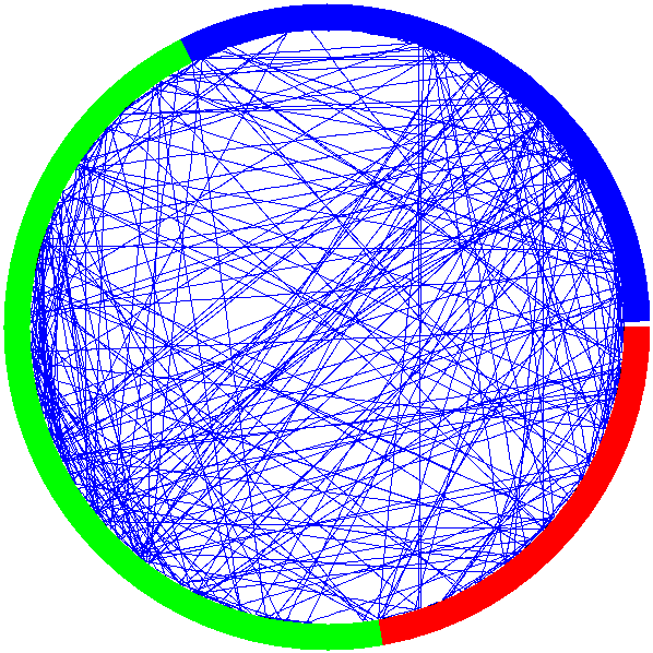
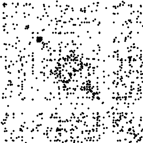
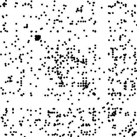
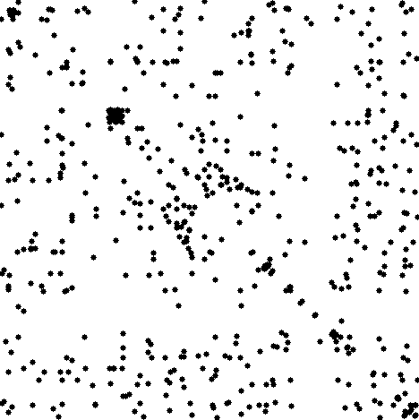
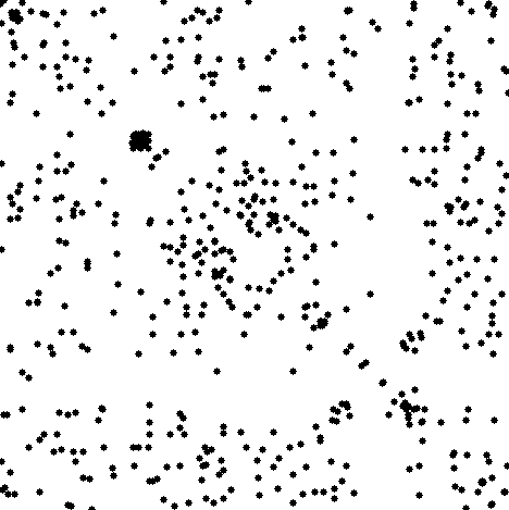
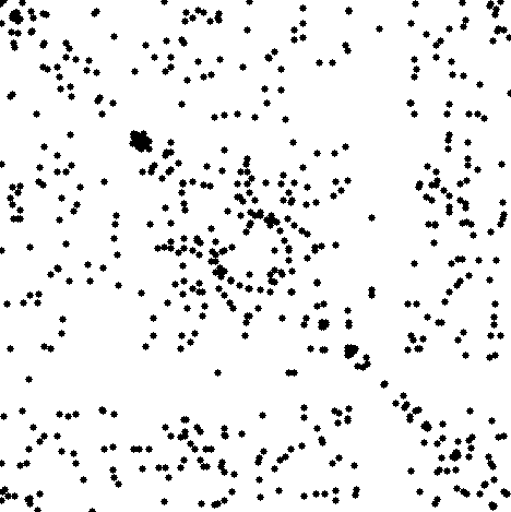
1	2	3	4	5	6
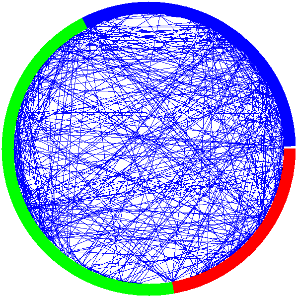
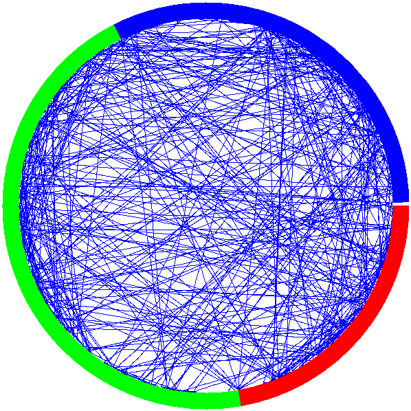
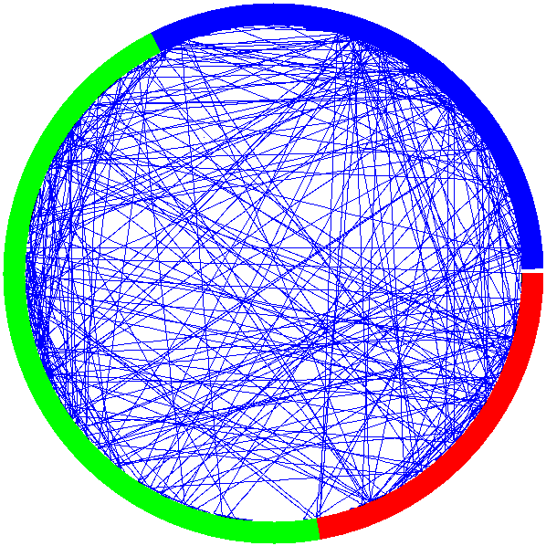
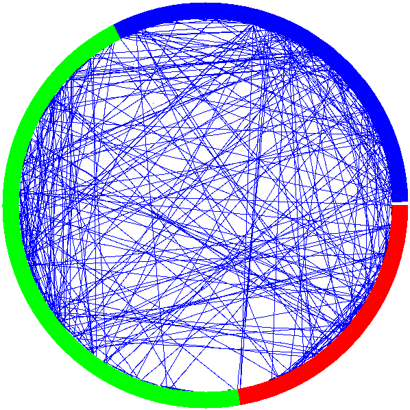
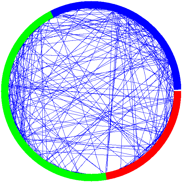
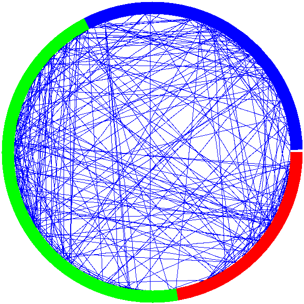
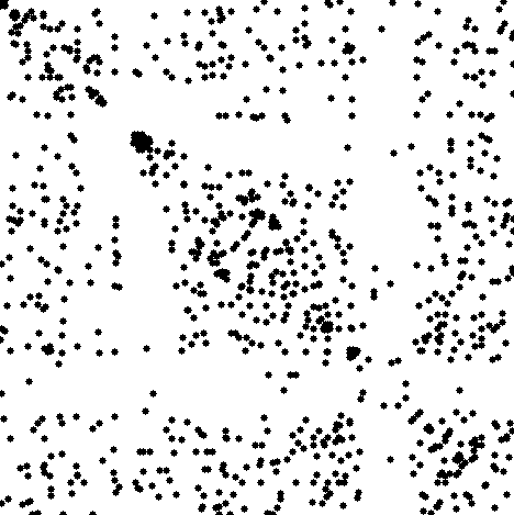
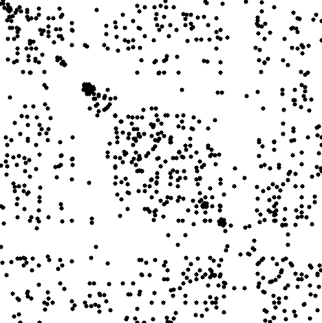
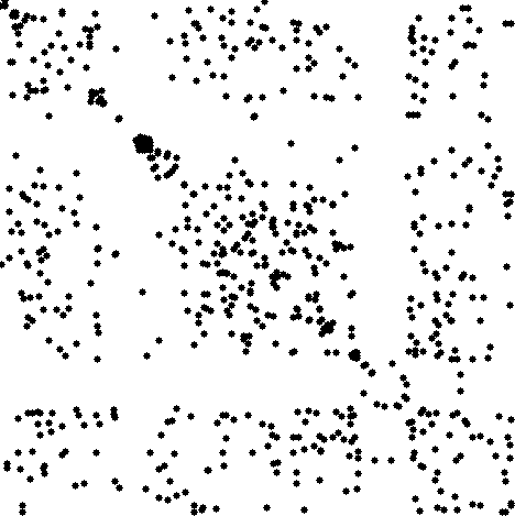
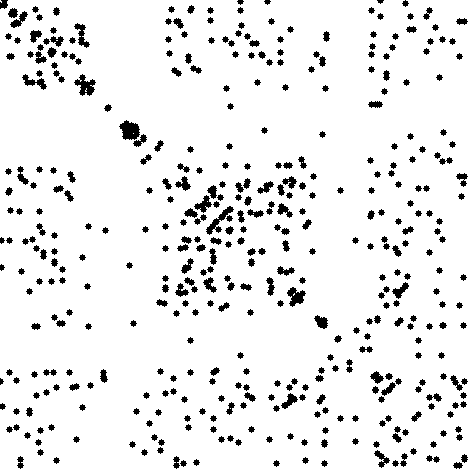
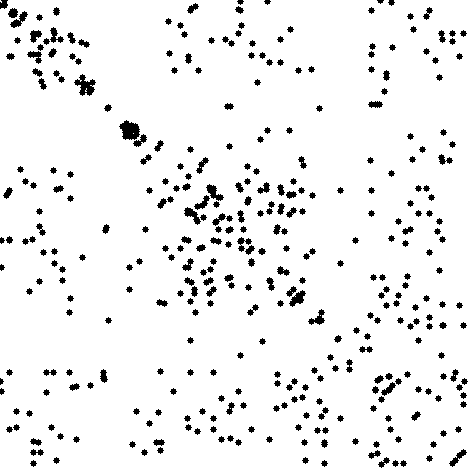
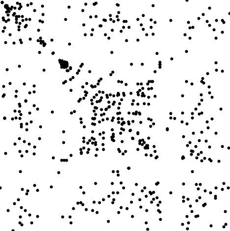
7	8	9	10	11	12	Visualization for the network at time point 4
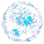
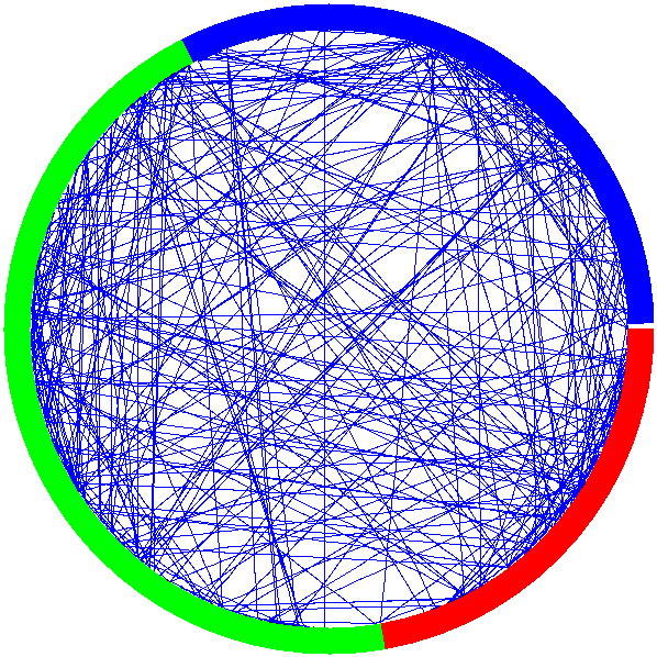
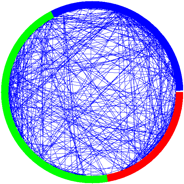
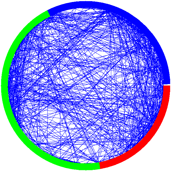
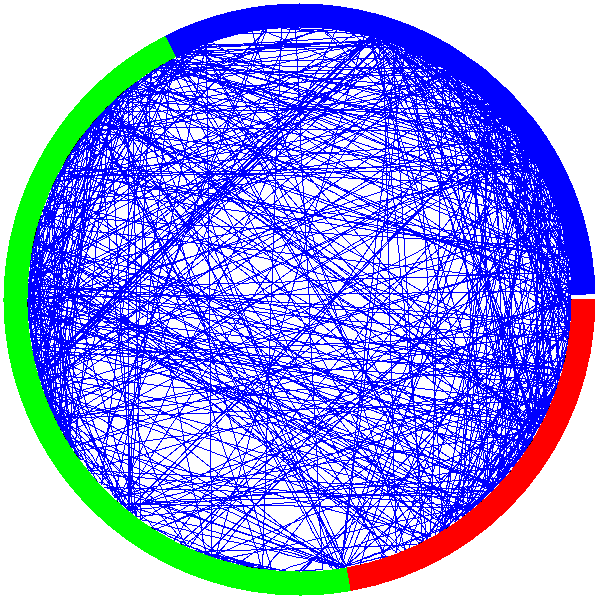
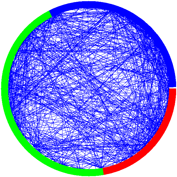
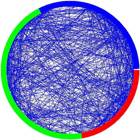
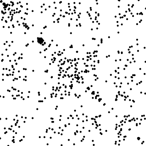
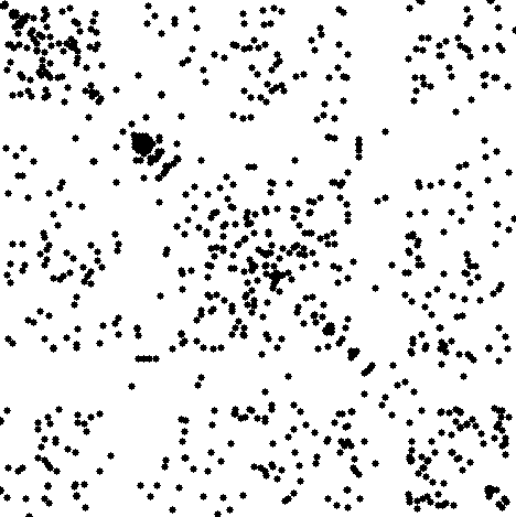
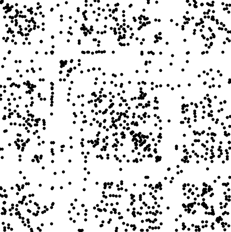
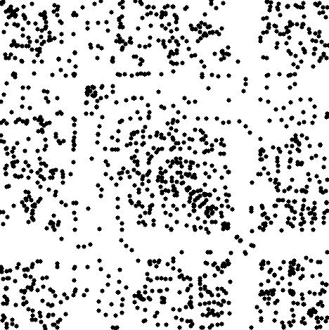
13	14	15	16	17	18
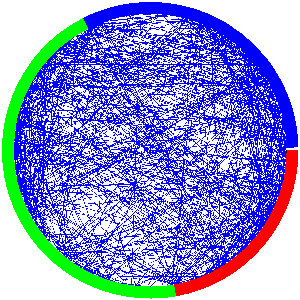
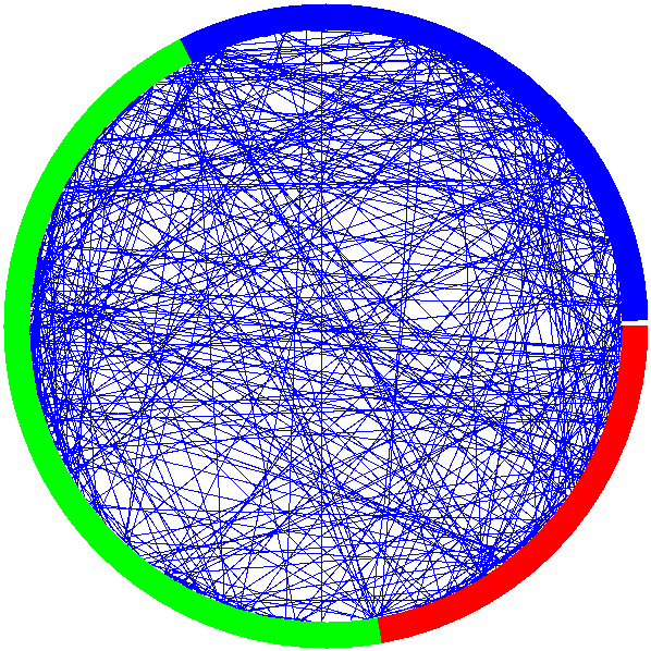
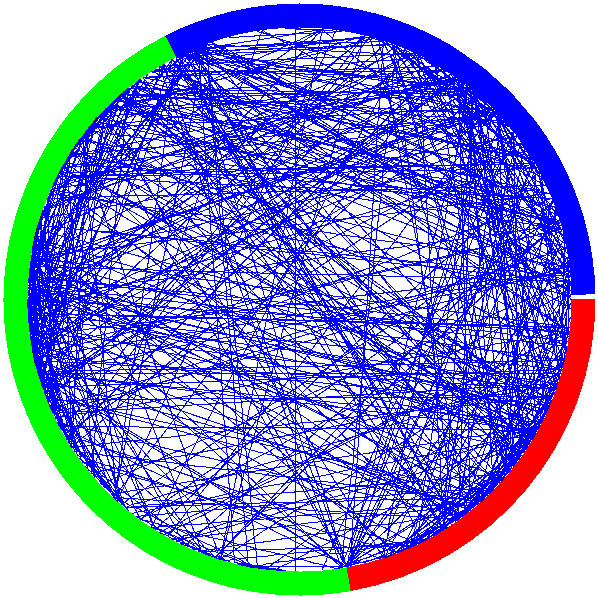
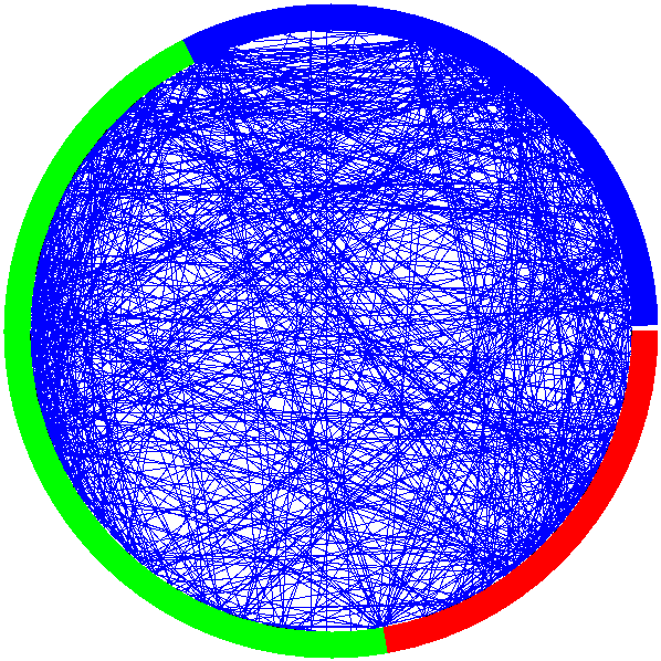
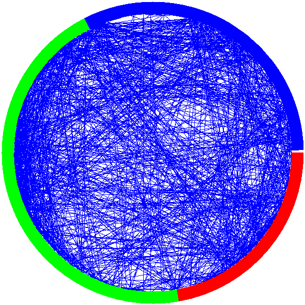
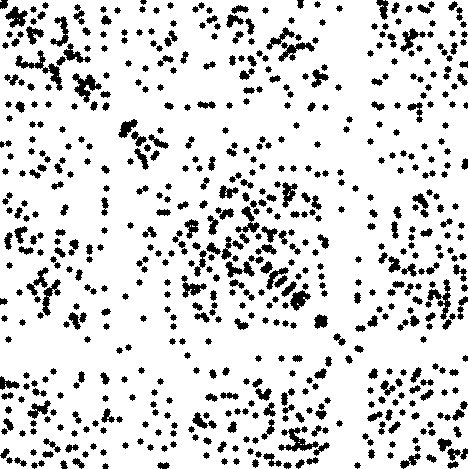
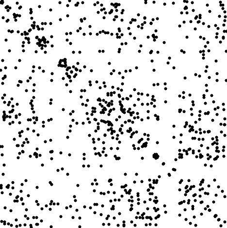
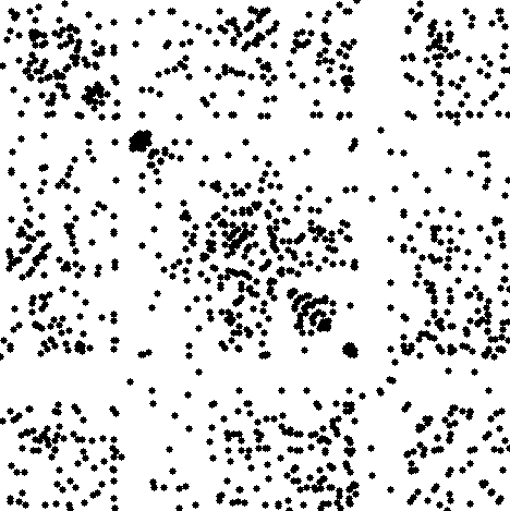
19	20	21	22	23		Visualization for the network at time point 23

Figure 1: The 23 snapshots of the dynamic networks are visualized using a circular layout and a scatter plot of the network adjacency matrix. For both layouts, genes are ordered according to their top level functions (either related to cellular component, molecular function or biological process). Furthermore, two snapshots are further visualized using a spring layout algorithm and displayed in the last column of the figure.

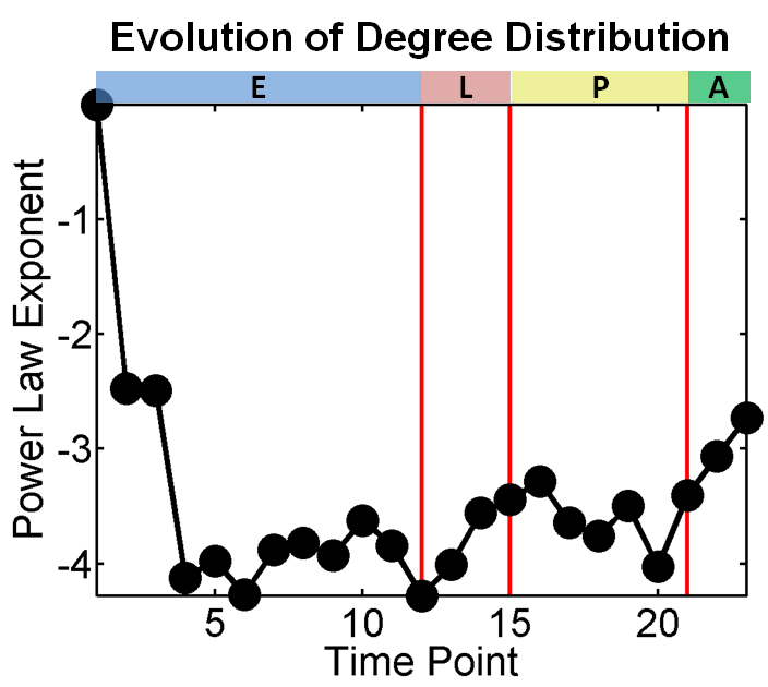
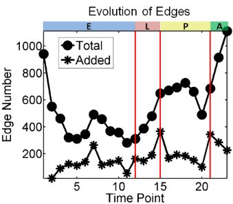
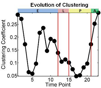
(a) (b) (c)

Figure 2: The evolution of the distribution on the node degree is summarized using its power law exponent in (a). The evolution of the number of edge is plotted in (b). The networks change in size over time with new edges appearing and old ones disappearing. The number of newly added edges in each time point is also plotted in (b). Plotted in (c) are the clustering coefficients for each snapshot of the temporal networks.

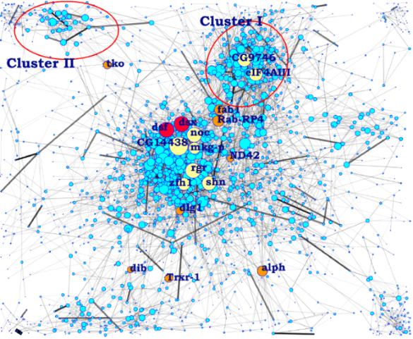
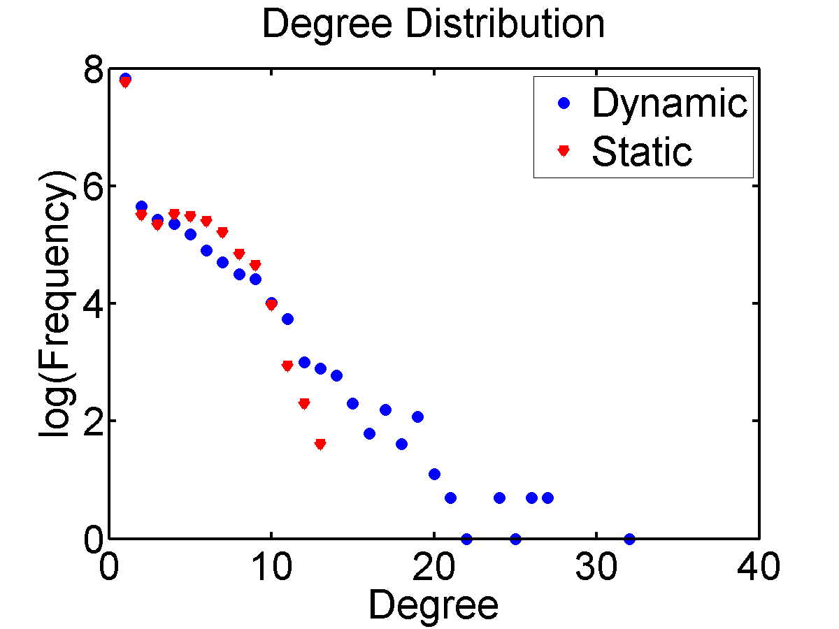
(a)
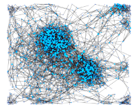
(b) (c)

Figure 3: The summary visualization in (a) is created by adding the 23-epoch dynamic networks together; the width of an edge is proportional to the number of times it occurs, and the size of a node is proportional to its degree. (b) A static network inferred by treating all microarray data as independently and identically distributed samples. (c) The degree distribution of the static network is different from that of the summary graph of the dynamic networks.

Hub Genes in the Dynamic Networks

The hub genes correspond to the high degree nodes in summary network. They represent the most influential elements of a network and tend to be essential for the developmental process of the organism. The top 50 hubs are identified from the summary graph of the dynamic networks in Fig. 3. These hubs are tracked over time in terms of their degrees and this evolution are visualized as colormap in Fig. 4(a).

To further understand the role played by these hubs, histogram analysis are performed on these 50 hubs in term of 43 ontological functions. The functional decomposition of these hubs are shown in Fig. 4(c). The majority of these hubs are related to functions such as binding and transcriptional regulation activity. This is in fact an expected outcome as transcription factors (TF) are thought to target a large number of genes and modulate their expression.

To further understand the functional spectrum of the genes targeted by the high degree transcriptional factors, the top 20 transcriptional factor hubs are also tracked over time in terms of their degrees and the evolution is illustrated in Fig. 4(b). The degrees of the transcriptional factors peak at different stages which means they differentially trigger target genes based on the biological requirements of developmental process. In Fig. 4(d)(e)(f), functional decomposition is performed on the target genes regulated by three example transcriptional factor hubs. For instance, peb, the protein ejaculatory bulb, interacts with extracellular region genes and genes involved in structural molecular activity. Another example is spt4 which triggers many binding genes. This is consistent with its functional role in chromatin binding and zinc ion binding.

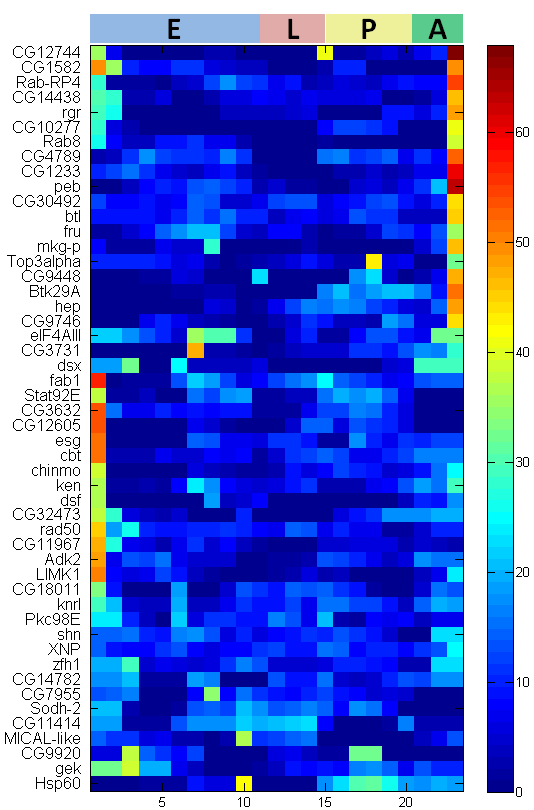
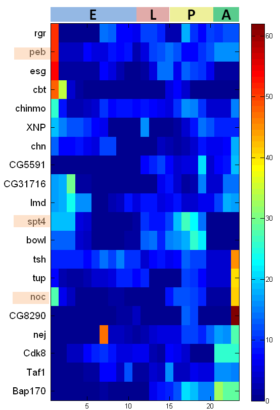
(a)	(b)
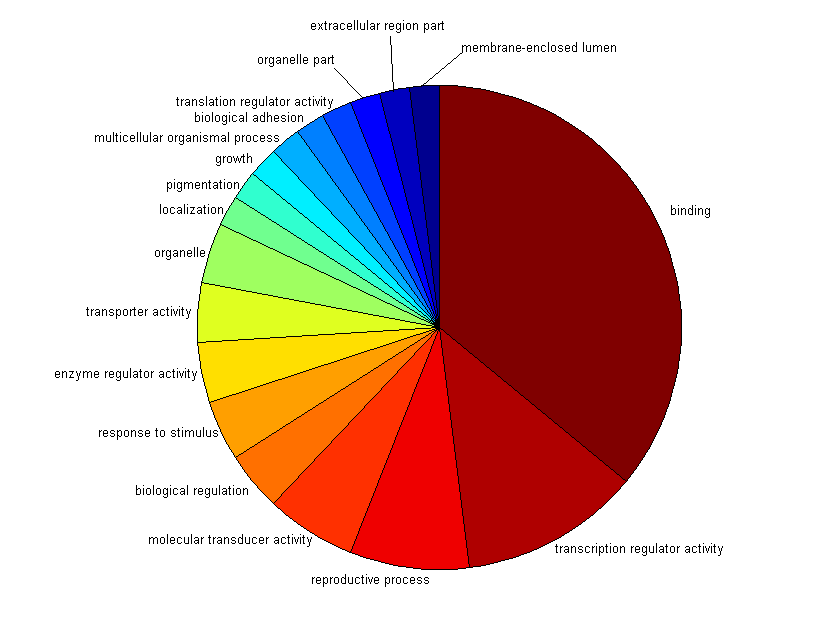
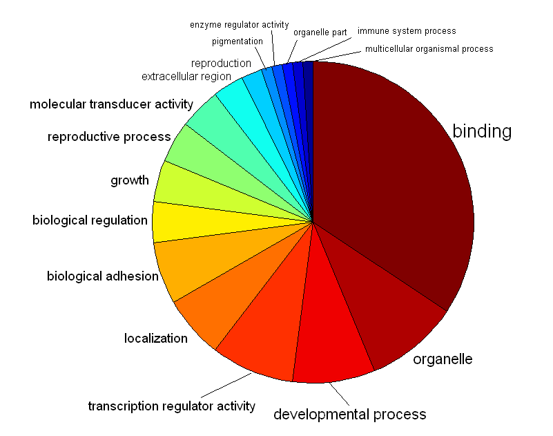
		(c)	(d)
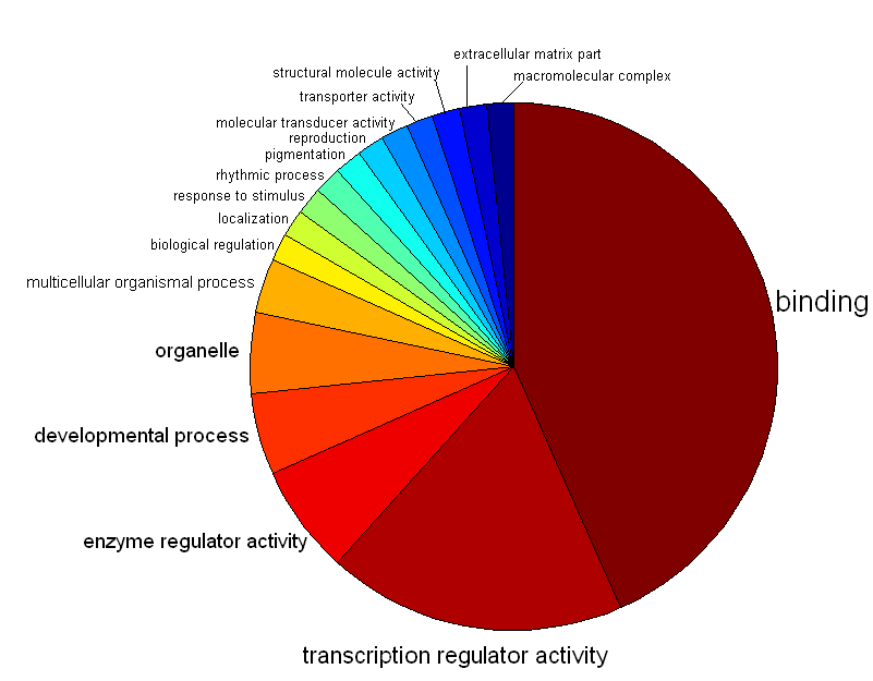
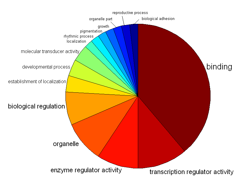
		(e)	(f)

Figure 4: (a) The top 50 hubs in the summary graph of the dynamic networks are tracked over time in terms of their degrees. Each row represents one hub and each column represents a time point with the color code corresponds to the degree of the hub. (b) shows the same information as (a) but only for the top 20 transcriptional factors with largest degree. (c) shows the functional decomposition of the top 50 hubs. (d)(e)(f) show examples of functional decomposition of the genes regulated by the transcriptional factor hub. These examples correspond to the highlighted gene in (b) and their gene names are peb, spt4 and noc respectively.

Dynamic Clustering of Genes

Most gene interactions occur only at certain time during the life cycle of Drosophila melanogaster. Indeed, on average there are only one eighth of the total gene interactions present in each temporal snapshot of the dynamic networks. The clusters in the summary graph are the result of temporal accumulation of the dynamic networks. To illustrate this, two clusters of genes are singled out from Fig 3(a) for further study. Cluster I consists of 167 genes and there are five major gene ontology groups, ie. binding activity (34.7%), organelle (9%), transporter activity (6.6%), transducer activity (6.6%) and motor activity (5.4%); cluster II consists of 90 genes and there are three major gene ontology groups, ie. structural molecule activity (61.1%), organelle (8.9%) and transporter activity (6.7%).

To obtain a finer functional decomposition of the genes in the interaction networks, the largest connected component of the summary graph is further grouped into 20 clusters. Although this connected component consists only of about 40% (1674) of all genes , it contains more than 97% (4401) of the interactions in the summary graph. This 20 clusters vary in size, with the smallest cluster having only 11 genes and the largest cluster having 384 genes. The evolution of these cluster of genes is illustrated in Fig. 5. It can be seen that the connections within a cluster dissolve and reappear over time, and different clusters wax and wane according to different schedule.

Furthermore, the functional composition of these 20 clusters are compared against the background functional composition of the set of all 4028 genes. For this purpose, gene ontology terms are used as the bins for the histogram, and the number of genes belonging to each ontology group are counted into the corresponding bins. The functional composition of 9 out of the 20 clusters are statistically significantly different from the background (two sample Kolmogorov-Smirnov test at significance level 0.05). The top 5 functional components of these significant clusters are summarized in Table 1.

Table 1: Top 5 functional components of the 9 clusters whose functional compositions are statistically significantly different from the back functional composition. The second column of the table displays the number of genes in each cluster respectively. The functional composition of each cluster is displayed as the percentage of genes with that particular function. The last column of the table shows that $p$-value of the statistical test.

#	Genes #	Top 5 Function Components	$p$-value
1	138	transcription regulator activity (15.9%), developmental process (8.7%),	$<10^{-6}$
		organelle (13.8%), reproduction (8.0%), localization (5.8%)
2	384	binding (37.8%), organelle (12.5%), transcription regulator activity (7.8%),	$<10^{-6}$
		enzyme regulator activity (7.6%), biological regulation (3.6%)
3	146	binding (29.5%), transporter activity (11.0%), organelle (8.9%),	$0.05$
		motor activity (6.2%), molecular transducer activity (5.5%)
4	120	structural molecule activity (45.0%), translation regulator activity (10.8%),	$<10^{-6}$
		organelle (6.7%), binding (5.8%), macromolecular complex (4.2%)
5	89	organelle (14.6%), binding (13.5%), multicellular organismal process (11.2%),	$10^{-3}$
		developmental process (7.9%), biological regulation (7.9%)
6	25	catalytic activity (16.0%), translation regulator activity (16.0%), organelle (8.0%),	0.04
		antioxidant activity (8.0%), cellular process (8.0%)
7	39	extracellular region (28.2%), biological adhesion (12.8%), binding (7.7%),	0.007
		reproduction (7.7%), transporter activity (5.1%)
8	119	multi-organism process (16.0%), reproduction (9.2%), developmental process (9.2%),	$<10^{-6}$
		molecular transducer activity (7.6%), organelle (5.9%)
9	151	binding (28.5%), envelope (14.6%), organelle (9.9%),	$<10^{-6}$
		organelle part (9.9%), transporter activity (5.3%)

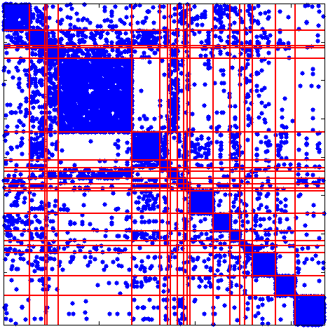
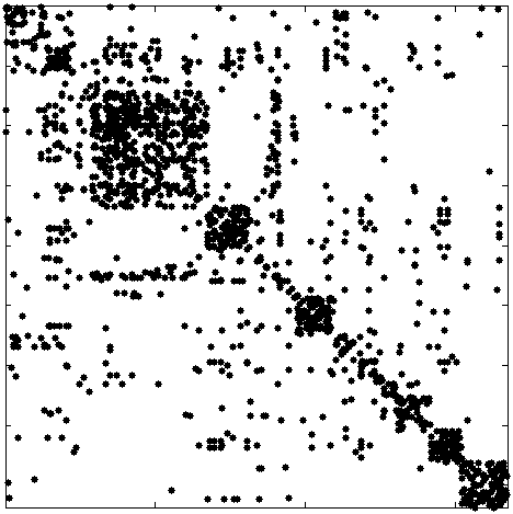
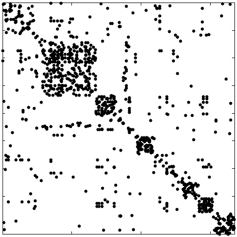
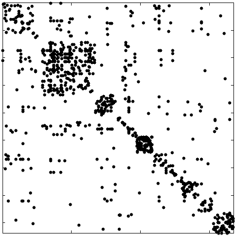
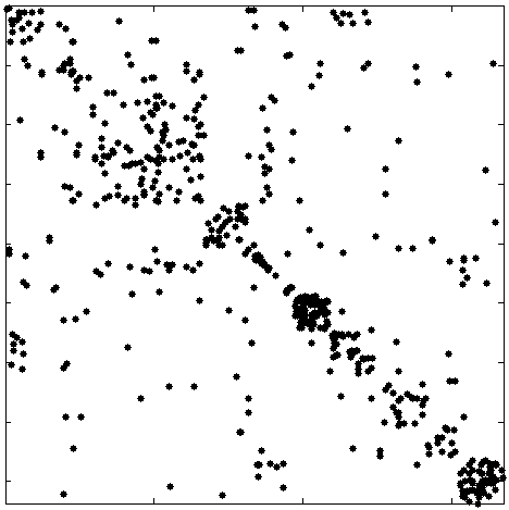
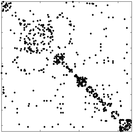
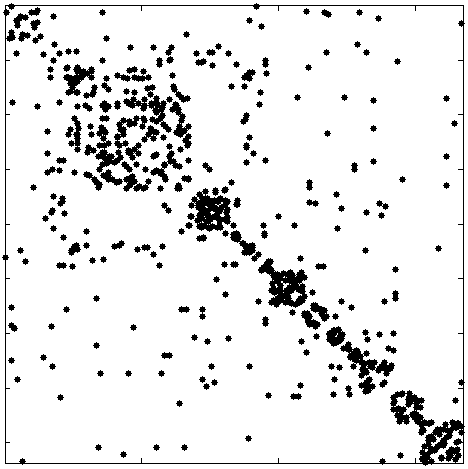
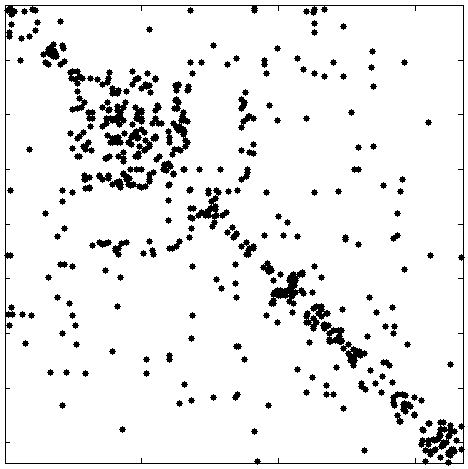
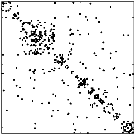
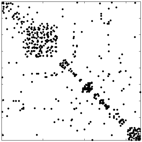
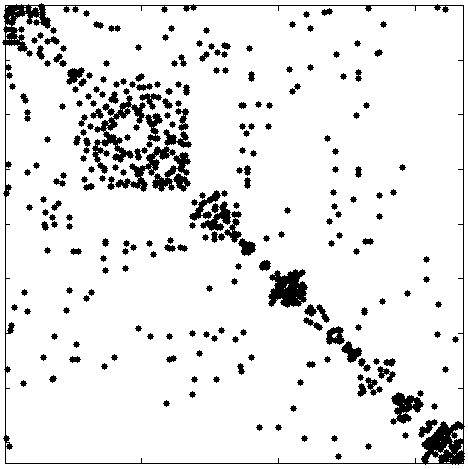
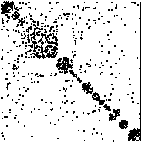
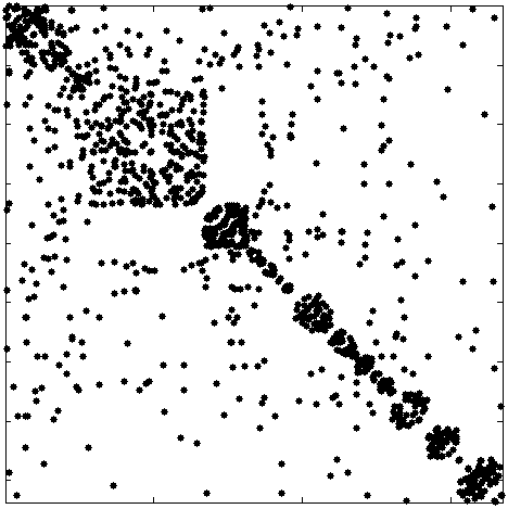
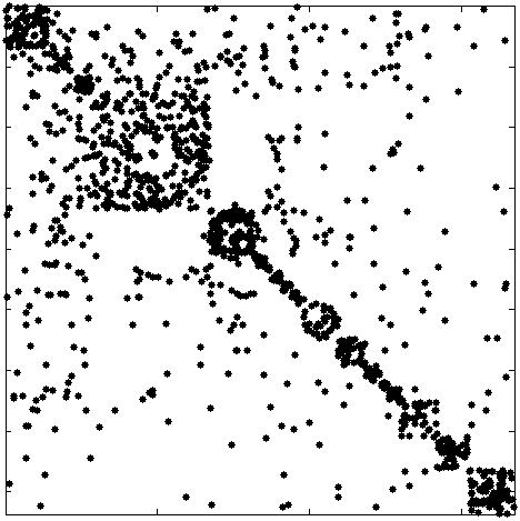
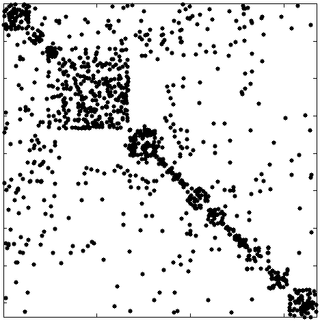
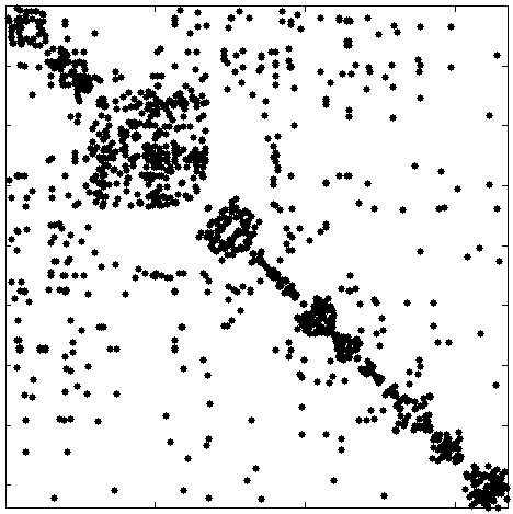
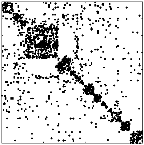
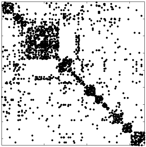
	1 2 3 4
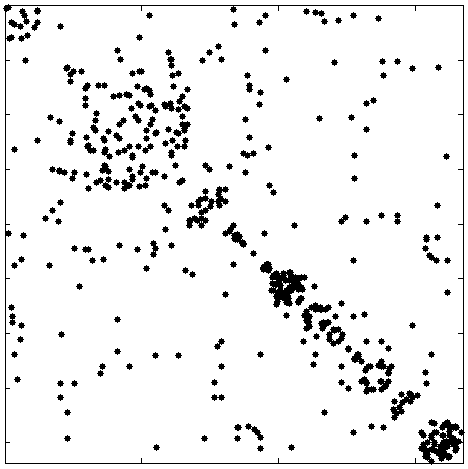
	5 6 7 8
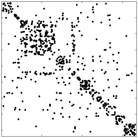
	9 10 11 12
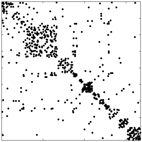
	13 14 15 16
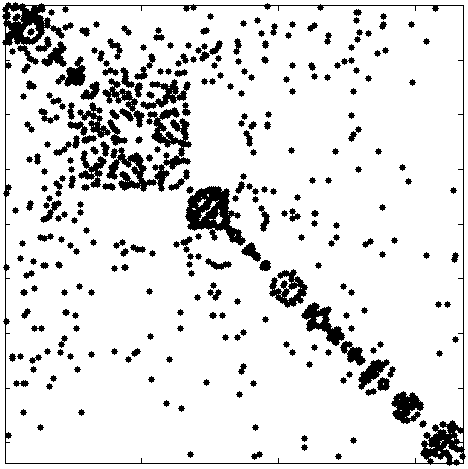
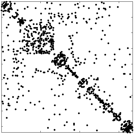
17 18 19	20 21 22 23

Figure 5: The adjacency matrix of the 20 clusters of genes derived from the largest connected components of Fig. 3 are plotted over time. Showed on the upper left corner is an enlarged picture of the adjacency matrix of the summary graph. The red lines show the boundaries between the clusters.

During the life cycle of Drosophila melanogaster, the developmental program of the organism may require genes related to one function be more active in certain stage than others. To investigate this, genes are grouped according to their ontological functions. It is expected that the interactions between gene ontology groups, as quantified by the number of wirings from genes in one group to those in another group, also exhibit temporal pattern of rewiring.

For this purpose, the 4028 genes are classified into 3 top level gene ontology (GO) groups related to cellular component, molecular function and biological process of Drosophila melanogaster according to Flybase. Then they are further divided into 43 gene ontology groups which are the direct children of the 3 top level GO groups. The interaction between these ontology groups evolving over time is shown in Fig. 6.

Through all stage of developmental process, genes belonging to three ontology groups are most active, and they are related to binding function, transcription regulator activity and organelle function respectively. Particularly, the group of genes involved in binding function play the central role as the hub of the networks of interactions between ontology groups. Genes related to transcriptional regulatory activity and organelles function show persistent interaction with the group of genes related to binding function. Other groups of genes that often interact with the binding genes are those related to functions such as developmental process, response to stimulus and biological regulation.

Large topological changes can also be observed from the temporal rewiring patterns between these gene ontology groups. The most diverse interactions between gene ontology groups occur at the beginning of embryonic stage and near the end of adulthood stage. In contrast, near the end of embryonic stage (time point 10), the interactions between genes are largely restricted to those from 4 gene ontology groups: transcriptional regulator activity, enzyme regulator activity, binding and organelle.

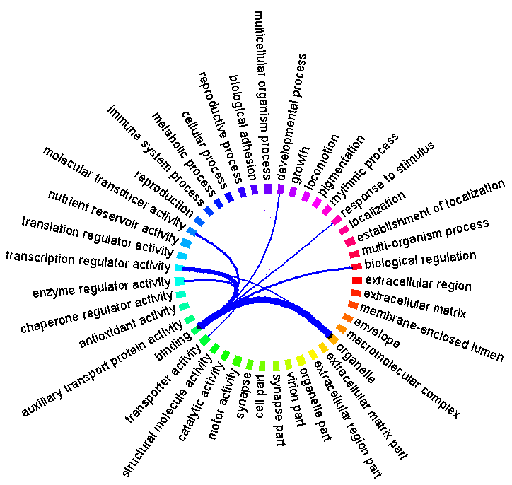
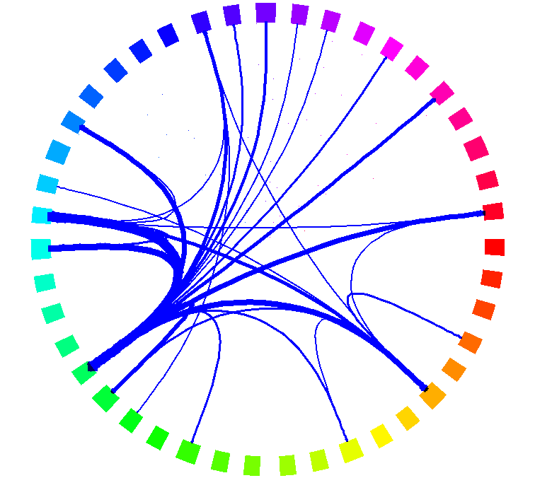
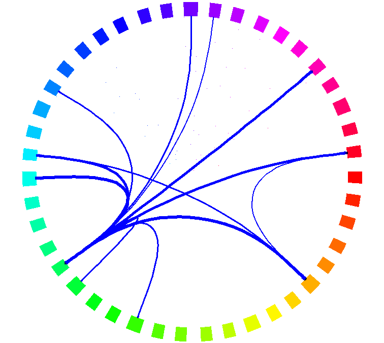
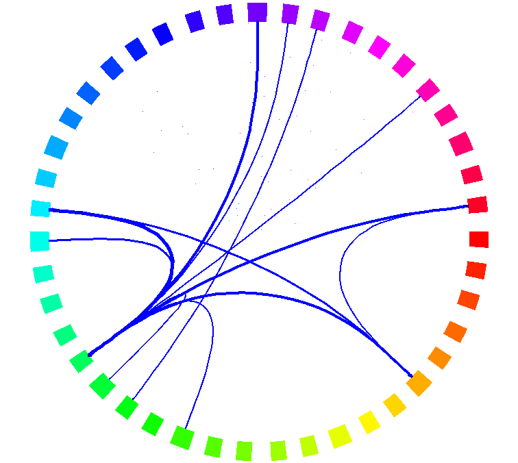
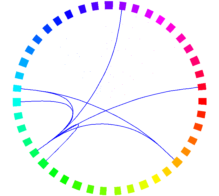
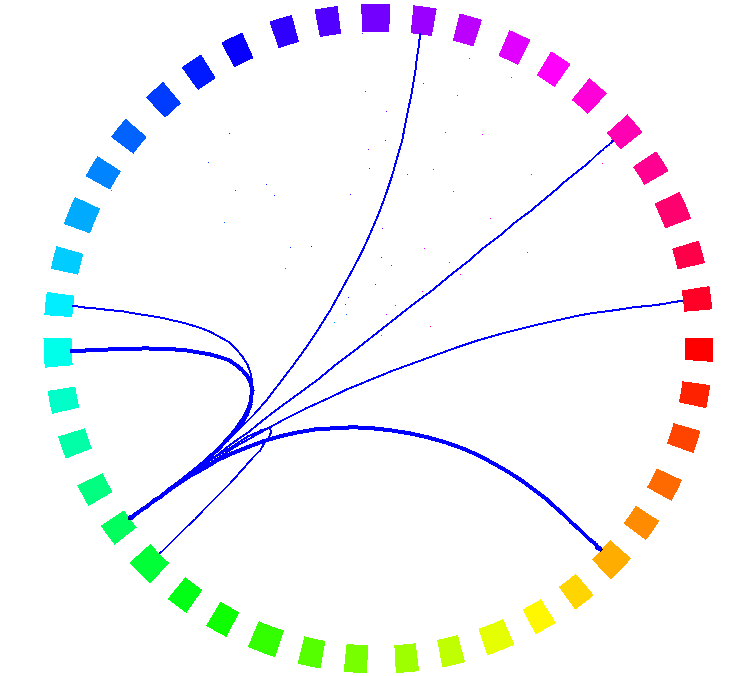
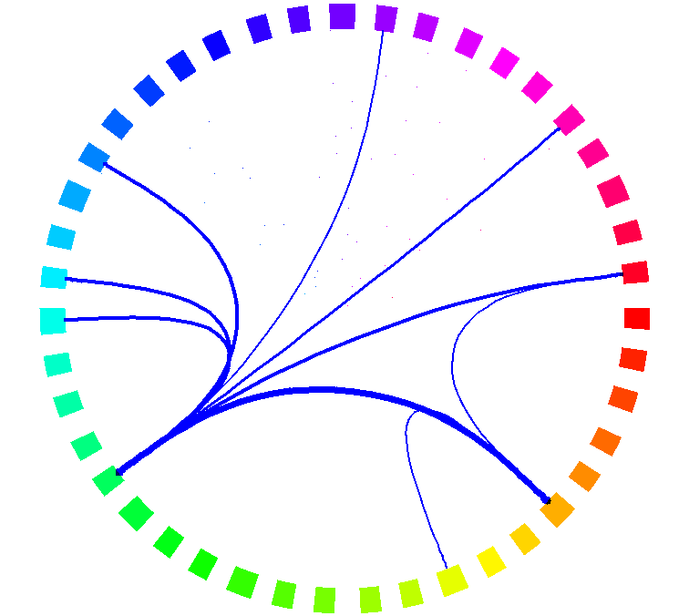
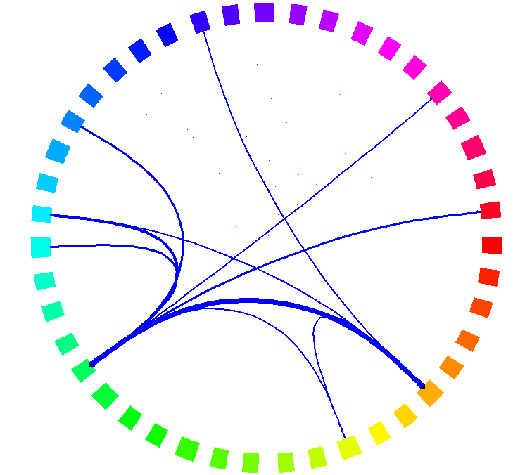
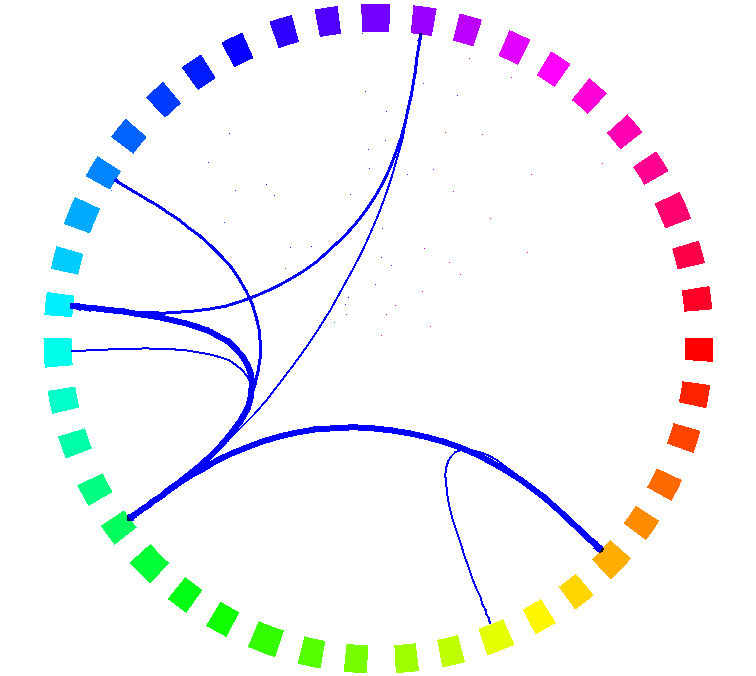
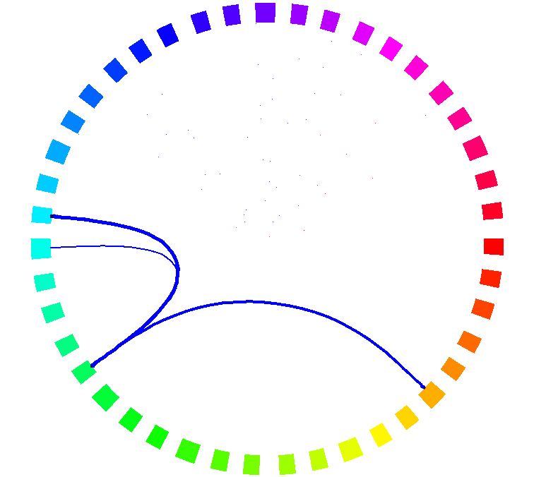
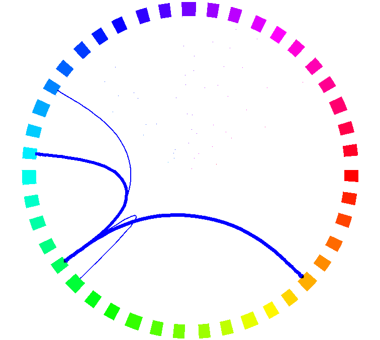
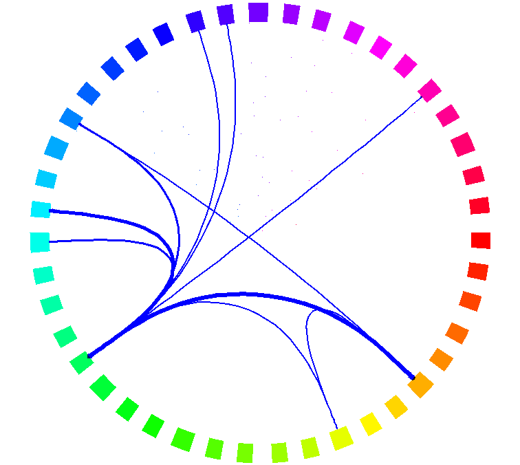
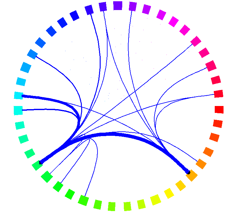
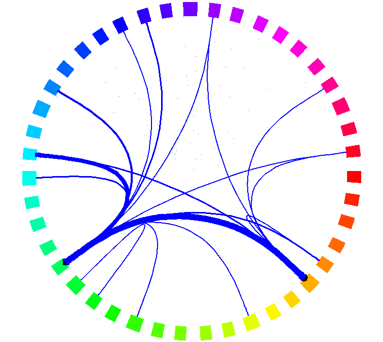
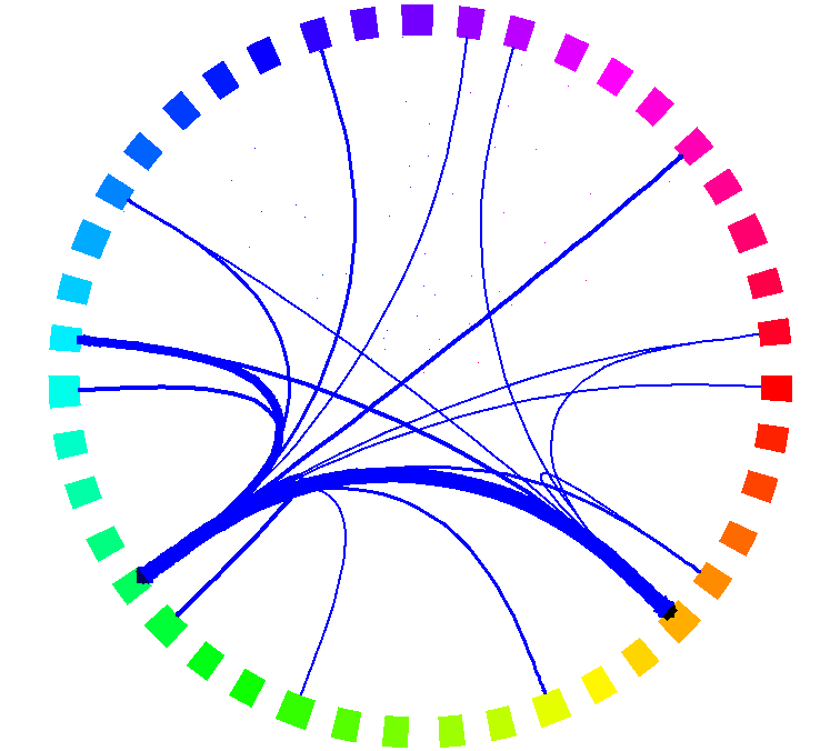
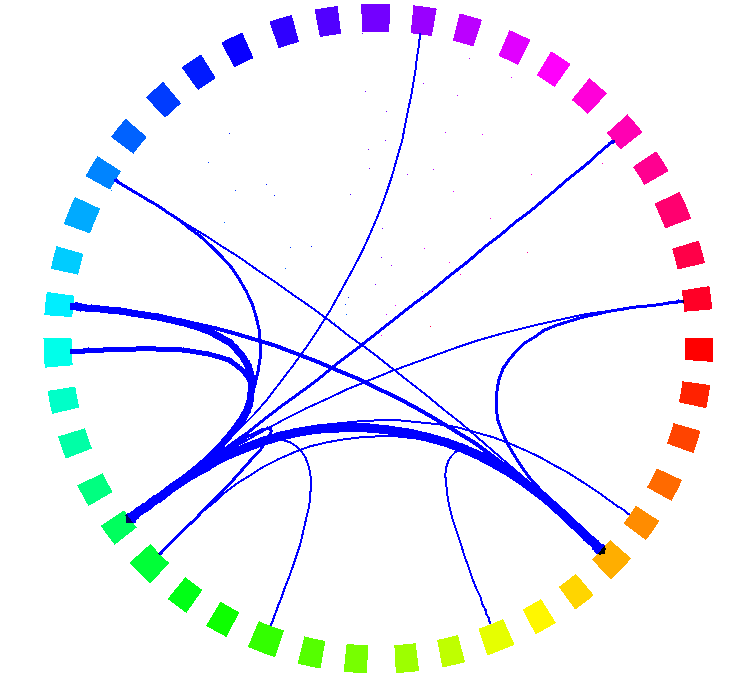
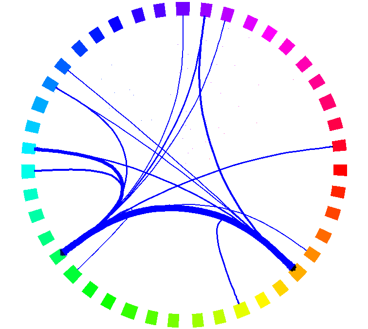
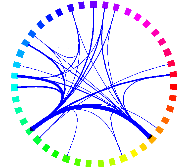
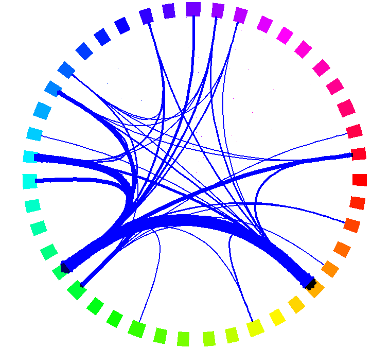
	1 2 3 4
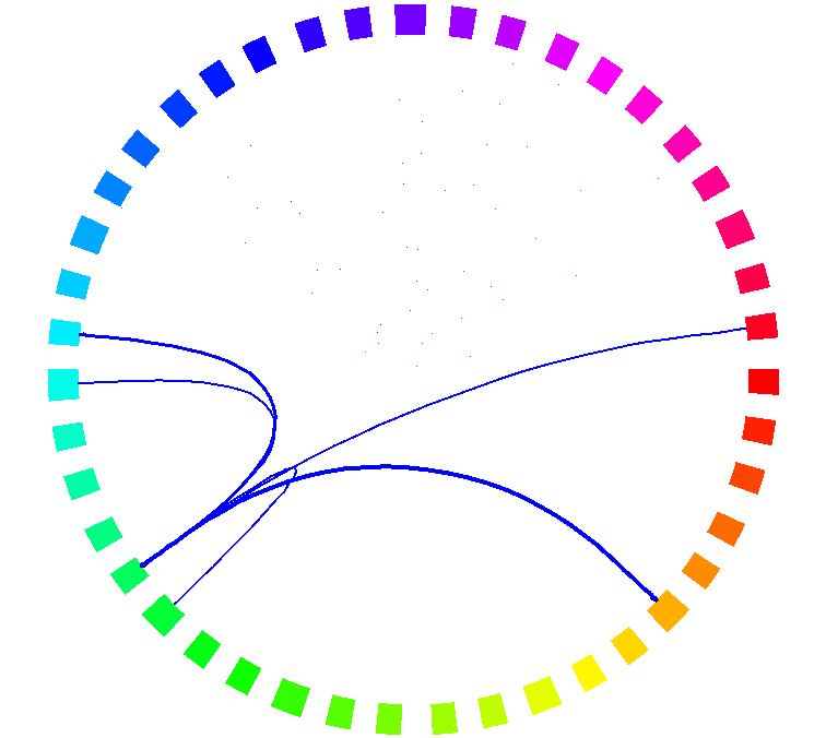
	5 6 7 8
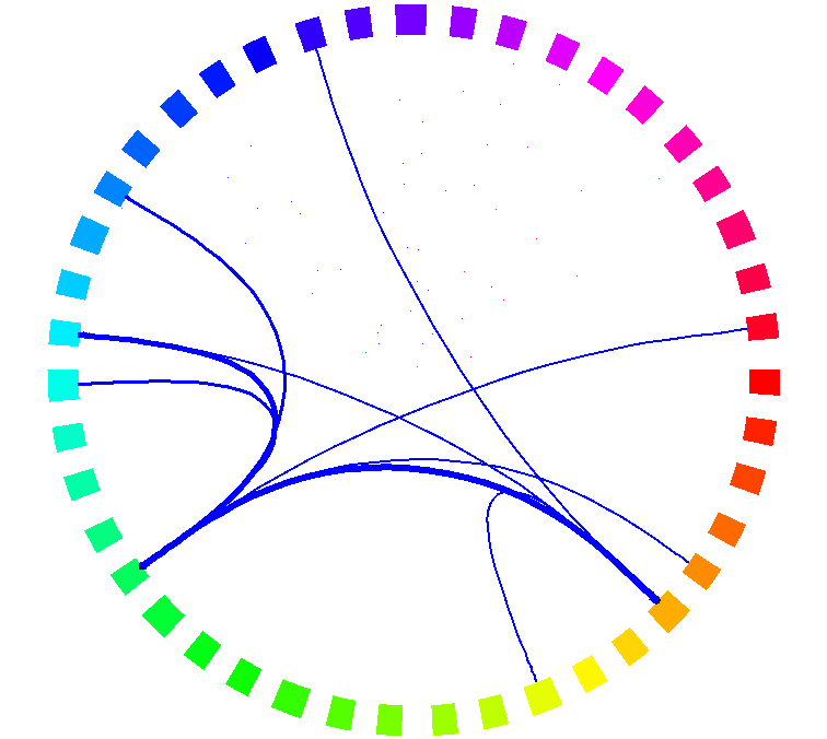
	9 10 11 12
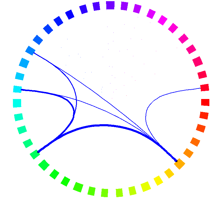
	13 14 15 16
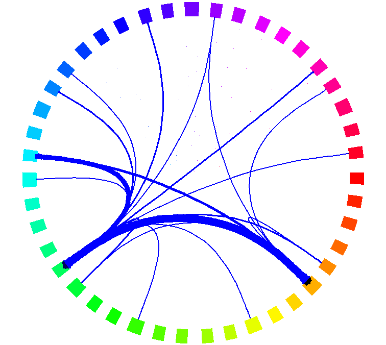
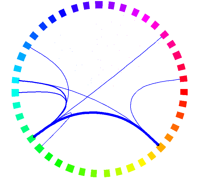
17 18 19	20 21 22 23

Figure 6: Temporally rewiring patterns of 43 gene ontology groups related to the cellular component, molecular function and biological process of Drosophila melanogaster. The 4028 measured genes are grouped according to the 43 ontology group; The weight of an edge between two ontology groups counts the number of connections between genes across these two groups. The width of an edge in the visualization is proportional to its weight. For clarity, only edges with weights greater than 5 are displayed. Each ontology group is coded in clockwise order with a color shown in the legend on the upper left corner.

Transient Coherent Subgraphs

During the development of Drosophila melanogaster, there may be sets of genes within which the interactions exhibit correlated appearance and disappearance. These sets of genes and their tight interactions form coherent subgraphs. Note that coherent subgraphs can be different from the clusters in the summary graph. While the former emphasizes the synchronous activation and deactivation of edges over time, the later only concerns the cumulative effect of the degree of interactions between genes.

To identify these coherent subgraphs, CODENSE (Hu et al., 2005) is applied to the inferred dynamic networks and 8 coherent subgraphs are discovered (Table 2). These coherent subgraphs vary in size, with the smallest subgraph containing 27 genes and the largest subgraph containing 87 genes. The degree of activity of these functional modules as measured by the clustering coefficients of the subgraphs follows a stage-specific temporal program. For instance, subgraph 3 and 4 are most active during the adulthood stage, while subgraph 4 and 7 are most active during embryonic and pupal stage respectively.

It is natural to ask whether the genes in a coherent subgraph are enriched with certain functions. To show this, the functional composition of these 6 subgraphs are also compared to the background functional composition of the set of all 4028 genes. Statistical test (two sample Kolmogorov-Smirnov test with significance level 0.05) shows that 6 out of the 8 subgraphs are significantly different from the background in term of their functions. For instance, subgraph 6 is enriched with genes related to binding (20.3%), envelope (18.6%), organelle part (16.9%), organelle (15.3%) and antioxidant activity (5.1%) ($p$-value $<10^{-6}$). Furthermore, these genes reveal increased activity near the end of the first 3 developmental stages. Another example is subgraph 7 which is enrich with genes related to transporter activity (11.1%), reproductive process (11.1%), multicellular organismal process (11.1%), organelle (7.4%) and transcription regulator activity (7.4%). These genes peak in their activity near the end of the pupal stage. These results suggest that different gene functional modules follow very different temporal programs.

Table 2: CODENSE is used to discover coherent subgraphs across the 23 temporally rewiring networks. Six such subgraphs are discovered. The number of genes within each subgraph are 69, 58, 29, 87, 64, 59, 27 and 63 respectively. In each cell of the table the evolution of the clustering coefficient for each subgraph is plotted, and the corresponding configurations of the subgraph at different time points are also illustrated.

1	2	3	4
5	6	7	8

Dynamics of Known Gene Interactions

Different gene interactions may following distinctive temporal programs of activation, appearing and disappearing at different time point during the life cycle of Drosophila melanogaster. In turn the transient nature of the interactions implies that the evidence supporting the presence of an interaction between two genes may not be present in all microarray experiments conducted during different developmental stages of the organism. Therefore, pooling all microarray measurements and inferring a single static network can undermine the inference process rather than helping it. This problem can be overcome by learning dynamic networks which recover transient interactions that are supported by correct subsets of experiments.

To show the advantage of dynamic networks over a static network, the recovered interaction by these two types of networks are compared against a list of 1143 known undirected gene interactions hosted in Flybase. The dynamic networks recover 96 of these known gene interactions while the static network only recovers 64. That is dynamic networks recover 50% more known gene interactions than the static network. Furthermore, the static network provides no information on when a gene interaction starts or ends. In contrast, the dynamic networks pinpoint the temporal on-and-off sequence for each recovered gene interaction.

To investigate whether the gene interactions with different activation pattern are related to their functional difference, hierarchical clustering is performed on these set of recovered gene interactions based on their activation patterns (Fig. 7). It can be seen that all these interactions are transient and very specific to certain stage of the life cycle of Drosophila melanogaster. Furthermore, gene interactions with similar activation pattern tends to recruit genes with similar functions. To demonstrate this, histogram analysis is performed base on the gene ontology groups of the genes involved in interactions. In Fig 7, five clusters in different level of the cluster hierarchy are highlighted and their histograms show that functionally different gene interactions tend to activation in very different temporal sequence. For instance, gene interactions in cluster I activates near the boundary of embryonic and larval stage, and in these interactions, no genes are related to the cellular component function of the organism; cluster II activates near the end of pupal stage and is enriched by genes related to the cellular component function.

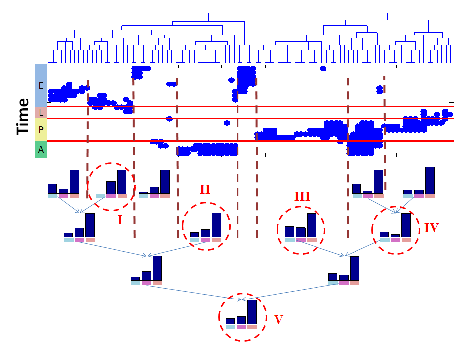
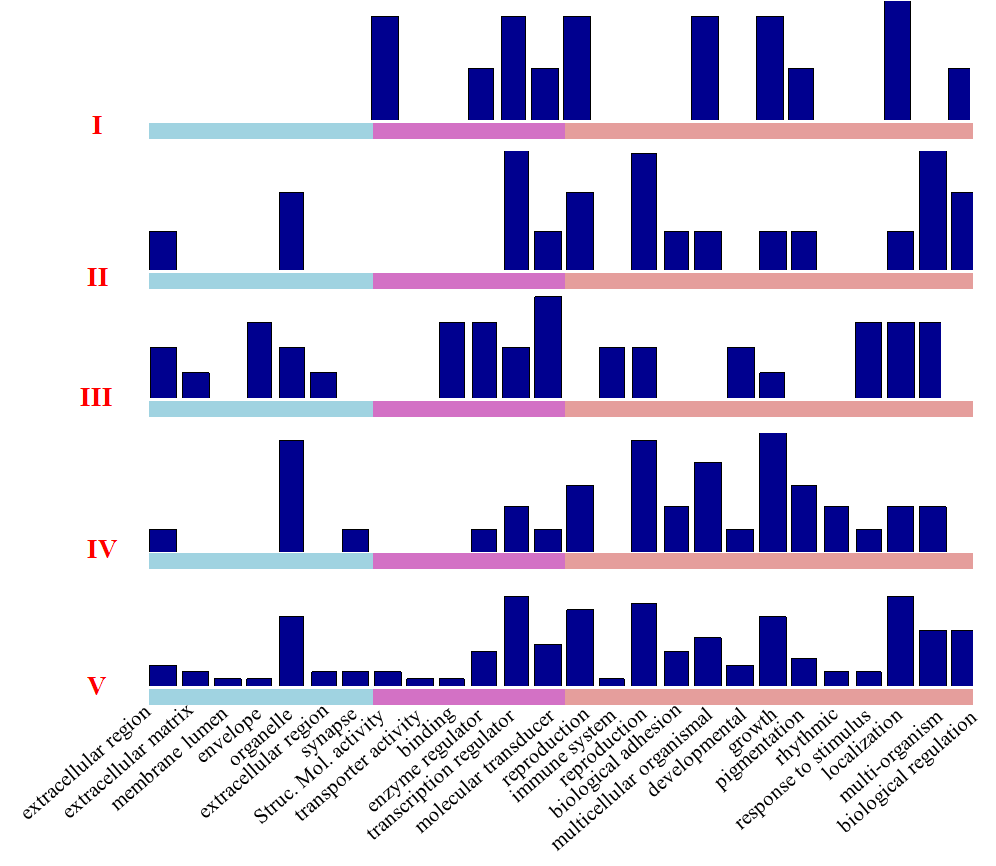
(a) (b)

Figure 7: Ninety six known gene interactions are recovered by the inferred dynamic networks. The onset and duration of these interactions follow different temporal patterns. The activation of each gene interaction over time is represented as one column in the upper part of (a); within each column, if a gene interaction is active a blue dot is drawn otherwise the space is left blank. These temporal sequences of activation can also be viewed as a sequence of zeros and ones where zero means not active and one means active. Based on these sequences of zeros and ones, hierarchical clustering is performed on the gene interactions. The clustering results are displayed on the top of the activation patterns. Note that the gene interactions have also been ordered according to the hierarchical clustering results. Therefore block of gene interactions with similar activation patterns can be seen. To investigate how the activation patterns of gene interactions are related to their biological function, several clusters of gene interactions are highlighted as cluster I, II, III IV and V. The 43 gene ontology terms are used as the bins to build histograms to investigate the functional composition of each cluster. The histograms are enlarged and shown in (b). The histogram bins are ordered according to the gene ontology groups shown in the horizontal axis. The colors of the axis indicate the top 3 level of the gene ontology group related to cellular component (cyan), molecular function (purple) and biological process (pink).

Conclusion

Numerous algorithms have been developed for inferring biological networks from high throughput experimental data, such as microarray profiles  (Segal et al., 2003; Dobra et al., 2004; Ong, 2002), ChIP-chip genome localization data (Lee et al., 2002; Bar-Joseph et al., 2003; Harbison et al., 2004), and protein-protein interaction (PPI) data (Uetz et al., 2000; Giot et al., 2003; Kelley et al., 2004; Causier, 2004), based on formalisms such as graph mining (Tanay et al., 2004), Bayesian networks (Cowell et al., 1999), and dynamic Bayesian networks (Kanazawa et al., 1995). However, most of this vast literature focused on modeling a static network or time-invariant networks  (Friedman et al., 2000), and much less has been done towards modeling the dynamic processes underlying networks that are topologically rewiring and semantically evolving over time, and on developing inference and learning techniques for recovering unobserved network topologies from observed attributes of entities (e.g., genes and proteins) constituting the network. The Tesla program presented here represents the first successful and practical tool for genome-wide reverse engineering the network dynamics based on the gene expression and ontology data. This method allows us to recover the wiring pattern of the genetic networks over a time series of arbitrary resolution. The recovered networks with this unprecedented resolution chart the onset and duration of many gene interactions which are missed by typical static network analysis. We expect collections of complex, high-dimensional, and feature- rich data from complex dynamic biological processes such as cancer progression, immune response, and developmental processes to continue to grow, given the rapid expansion of categorization and characterization of biological samples, and the improved data collection technologies. Thus we believe our new method is a timely contribution that can narrow the gap between imminent methodological needs and the available data, and offer deeper understanding of the mechanisms and processes underlying biological networks.

Material and Methods

Microarray Data

We used the microarray data collected by Arbeitman et al. (2002) in their study of the gene expression patterns during the life cycle of Drosophila melanogaster. Approximately 9,700 Drosophila cDNA elements representing 5,081 different genes were used to construct the 2-color spotted cDNA microarrays. The genes analyzed in this paper consists of a subset of 4,028 sequence-verified, unique genes. Experimental samples were measured at 66 different time points spanning the embryonic, larval, pupal and adulthood period. Each hybridization is a comparison of one sample to a common reference sample made from pooled mRNA representing all stages of the life cycle. Normalization is performed so that the dye dependent intenstive response is removed and the average ratio of signals from the experimental and reference sample equals one. The final expression value is the log ratio of signals.

Missing Value Imputation

Missing values are imputed in the same manner as Zhao et al. (2006). This is based on the assumption that gene expression values change smoothly over time. If there is a missing value, a simple linear interpolation using values from adjacent time points is used, i.e. the value of the missed time point is set to the mean of its two neighbors. When the missing point is a start or a end point, it is simply filled with the value of its nearest neighbor.

Expression Value Binarization

The expression values are quantized into binary numbers using thresholds specific to each gene in the same manner as Zhao et al. (2006). For each gene, the expression values are first sorted; then the top two extreme values in either end of the sorted list are discarded; last the median of the remaining values are used as the threshold above which the value is binarized as 1 and 0 otherwise. Here 1 means the expression of a gene is up-regulated, and 0 means down-regulated.

Network Inference model

In this paper, we used a new approach for recovering time-evolving networks on fixed set of genes from time series of gene expression measurements using temporally smoothed $L_{1}$-regularized logistic regression, or in short, TLR (for temporal LR). This TLR can be formulated and solved using existing efficient convex optimization techniques which makes it readily scalable to learning evolving graphs on a genome scale over few thousands of genes.

For each time epoch we assumed that we observe binary gene activation patterns, which we obtained from the continuous micro-array measurements as described above. At each epoch we represent the regulatory network using a Markov random field define as follows:

Let $G^{t}=(V,E^{t})$ be the graph structure at time epoch $t$ with vertex set $V$ of size $|V|$ = p and edge set $E^{t}$. Let $\{X^{t}_{1:N_{t}}\}$ be a set of i.i.d binary random variables associated with the vertices of the graph. Let the joint probability of the random variables be given by the Ising model as follows:

$$P(\mathbf{x^{t}_{d}}|\Theta^{t}) = {\rm{exp}}\Bigg{(}\sum_{i\in V}{\theta^{t}_{ii}x_{d,i}^{t}}+\sum_{(i,j)\in E^{t}}{\theta^{t}_{ij}x^{t}_{d,i}x^{t}_{d,j}-A(\Theta^{t})}\Bigg{)},$$ (1)

where the parameters $\{\theta^{t}_{ij}\}_{(i,j)\in E^{t}}$ capture the correlation (regulation strength) between genes $X^{t}_{i}$, and $X^{t}_{j}$. $A(\Theta^{t})$ is the log normalizing constant of the distribution. Given a set of $\{X^{t}_{1:N_{t}}\}$ i.i.d samples drawn from $P(X^{t}_{d}|\Theta^{t})$ at each time step, the goal is to estimate the structure of the graph, i.e. to estimate $\{\hat{E^{t}}\}_{t=1}^{T}$. We cast this problem as a regularized estimation problem of the time-varying parameters of the graph as follows:

$$\hat{\Theta^{1}},\ldots,\hat{\Theta^{T}} = \arg\min_{\Theta^{1},\ldots,\Theta^{T}}\,\,\,\sum_{t=1}^{T}{nLL(\Theta^{t})}\,\,+\,\,R(\Theta^{1}\ldots\Theta^{T},\lambda),$$ (2)

where, $nLL(\cdot)$ is the exact (or approximate surrogate) of the negative Log Likelihood $R(\cdot)$ is a regularization term, and $\lambda$ is the regularization parameter(s). We assume that the graph is sparse and evolves smoothly over time, and we would like to pick a regularization function $R(\cdot)$ that results in a sparse and smooth graphs. The structure of the graphs can then be recovered from the non-zero parameters which are isomorphic to the edge set of the graphs.

When $T=1$, the problem in Eq. (2) degenerates to the static case:

$$\hat{\Theta} = \arg\min_{\Theta}\,nLL(\Theta)+R(\Theta,\lambda),$$ (3)

and thus one needs only to use a regularization function, $R(\cdot)$, that enforces sparsity. Several approaches were proposed in the literature (Wainwright et al., 2006; Lee et al., 2006; Guo et al., 2007). this problem has been addressed by choosing $R=L_{1}$-penalty, however, they differ in the way they approximate the first term in Eq. (3) which is intractable in general due to the existence of the log partition function, $A(\Theta)$ (Wainwright et al., 2006; Lee et al., 2006; Guo et al., 2007). In Wainwright et al. (2006) a pseudo-likelihood approach was used. The pseudo-likelihood, $\hat{P}(X_{d}|\Theta)=\prod_{i=1}^{P}{P\big{(}x_{d,i}|\mathbf{x_{d,N(i)}}\big{)}}$, where $N(i)$ is the Markov blanket of node $i$, i.e., the neighboring nodes of node $i$. In the binary pairwise-MRF, this local likelihood has a logistic-regression form. Thus the learning problem in (3) degenerates to solving $P$ $l_{1}$-regularized logistic regression problems resulting from regressing each individual variable on all the other variables in the graph. More specifically, the learning problem for node $i$ is given by:

$$\hat{\mathbf{\theta}_{i}} = \arg\min_{\theta_{i}}\frac{1}{N}\sum^{N}_{d=1}{\log\,P\big{(}x_{d,i}|\mathbf{x_{d,-i}},\theta_{i}\big{)}}+\lambda_{1}\parallel\theta_{-i}\parallel_{1}$$ (4)

$$= \arg\min_{\mathbf{\theta_{i}}}\frac{1}{N}\sum^{N}_{d=1}{\big{[}\mathrm{log}(1+\mathrm{exp}(\mathbf{\theta_{i}}\mathbf{x_{d,-i})})-x_{d,i}\mathbf{\theta_{i}}\mathbf{x_{d,-i}}\big{]}}+\lambda_{1}\parallel\mathbf{\theta_{-i}}\parallel_{1},$$

where, $\mathbf{\theta_{i}}=(\theta_{i1},\ldots,\theta_{iP})$ are the parameters of the $L_{1}$-logistic regression, $\mathbf{x_{d,-i}}$ denotes the set of all variables with $x_{d,i}$ replaced by 1, and $\theta_{-i}$ denotes the vector $\theta_{i}$ with the component $\theta_{ii}$ removed (i.e. the intercept is not penalized). The estimated set of neighbors is given by: $\hat{N}(i)=\{j:\theta_{ij}\neq 0\}$. The set of edges $E$ is then defined as either a union or an intersection of neighborhood sets $\{N(i)\}_{i\in V}$ of all the vertices. Wainwright et al. (2006) showed that both definitions would converge to the true structure asymptotically.

To extend the above approach to the dynamic setting, we return to the original learning problem in Eq. (2) and approach it using the techniques presented above. We use the negative pseudo-loglikelihood as a surrogate for the intractable $nLL(\cdot)$ at each time epoch. To constrain the multiple time-specific regression problems each of which takes the form of Eq. (4) so that graphs are evolving in a smooth fashion, that is, not dramatically rewiring over time, we penalize the difference between the regression coefficient vectors corresponding to the same node, say $i$, at the two adjacent time steps. This can be done by introducing a regularization term $\parallel\theta_{i}^{t}-\theta_{i}^{t-1}\parallel_{1}^{1}$ for each node at each time. Then, to also enforce sparsity over the graphs learnt at each epoch, in addition to the smoothness between their evolution across epochs, we use the standard $L_{1}$ penalty over each $\theta_{i}^{t}$. These choices will decouple the learning problem in (2) into a set of $P$ separate smoothed $L_{1}$-regularized logistic regression problems, one for each variable. Putting everything together, for each node $i$ in the graph, we solve the following problem for :

$$\hat{\theta}_{i}^{1},\ldots,\hat{\theta}_{i}^{T} = \arg\min_{\theta_{i}^{1},\ldots,\theta_{i}^{T}}\sum^{T}_{t=1}{l_{avg}(\theta_{i}^{t})}+\lambda_{1}\sum^{T}_{t=1}{\parallel\theta_{-i}^{t}\parallel_{1}}+\lambda_{2}\sum^{T}_{t=2}{\parallel\theta_{i}^{t}-\theta_{i}^{t-1}\parallel_{1}^{1}},\,\,\,$$ (5)

where

$$\,\,l_{avg}(\mathbf{\theta_{i}^{t}}) = \frac{1}{N^{t}}\sum^{N^{t}}_{d=1}{\log\,P\big{(}x^{t}_{d,i}|\mathbf{x^{t}_{d,-i}},\mathbf{\theta^{t}_{i}}\big{)}}$$ (6)

$$= \frac{1}{N^{t}}\sum^{N^{t}}_{d=1}{\big{[}\mathrm{log}(1+\mathrm{exp}(\mathbf{\theta^{t}_{i}}\mathbf{x^{t}_{d,-i}}))-x^{t}_{d,i}\mathbf{\theta^{t}_{i}}\mathbf{x^{t}_{d,-i}}\big{]}}.$$

The problem in Eq. (5) is a convex optimization problem with a non-smooth $L_{1}$ functions. Therefore, we solve the following equivalent problem instead by introducing new auxiliary variables, $\mathbf{u^{t}_{i}}$ and $\mathbf{v^{t}_{i}}$ (the case for $q=2$ is handled similarly):

$$\min_{\theta_{i}^{1},\ldots,\theta_{i}^{T},u_{i}^{1},\ldots,u_{i}^{T},v_{i}^{2},\ldots,v_{i}^{T}}\sum^{T}_{t=1}{l_{avg}(\theta_{i}^{t})}+\lambda_{1}\sum^{T}_{t=1}\mathbf{1}^{T}{\mathbf{u^{t}_{i}}}+\lambda_{2}\sum^{T}_{t=2}{\mathbf{1}^{T}\mathbf{v^{t}_{i}}}$$ (7)

$$\mathrm{subject\,to}\quad-u^{t}_{i,j}\leq\theta^{t}_{i,j}\leq u^{t}_{i,j},\,\,t=1,\ldots,T,j=1,\ldots,i-1,i+1,\ldots,P,$$

$$\mathrm{subject\,to}\quad-v^{t}_{i,j}\leq\theta^{t}_{i,j}-\theta^{t-1}_{i,j}\leq v^{t}_{i,j},\,\,t=2,\ldots,T,j=1,\ldots,P,$$

where $\mathbf{1}$ denotes a vector with all components set to 1, so $\mathbf{1}^{T}\mathbf{u^{t}_{i}}$ is the sum of the components of $\mathbf{u^{t}_{i}}$. To see the equivalence of the problem in Eq. (7) with the one in Eq. (5, we note that at the optimal point of Eq. (7), we must have $u^{t}_{i,j}=|\theta^{t}_{i,j}|$, and similarly $v^{t}_{i,j}=|\theta^{t}_{i,j}-\theta^{t-1}_{i,j}|$, in which case the objectives in Eq. (7) and Eq. (5) are the same (a similar solution has been applied to solving $L_{1}$-regularized logistic regression in Koh et al. (2007)). The problem in Eq. (7) is a convex optimization problem, with now a smooth objective, and linear constraint functions, so it can be solved by standard convex optimization methods, such as interior point methods, and high quality solvers can directly handle the problem in Eq. (7) efficiently for medium to large scale (up to few thousands of nodes). In this paper, we used the CVX optimization package.

Gene Ontology

Gene ontology (GO) data is obtained from Flybase. There are altogether 25,072 GO terms with 3 name spaces: molecular function, biological process and cellular component. The GO terms are organized into a hierarchical structure, and 16,189 GO terms are leaf nodes of the hierarchy. The 4,028 genes are assigned to one or more leaf nodes. When we estimate the networks for a target gene, we restrict the network inference to those genes that share common GO terms with the target gene. This operation restricts the network inference to a biologically plausible set of genes and it also drastically reduces the computation time.

Mining Frequent Coherent Subgraphs

CODENSE is an algorithm for efficiently mining frequent coherent dense subgraphs across a large number of massive graphs (Hu et al., 2005). In the context of dynamic networks, it is adapted to discover functionally coherent gene modules across the temporal snapshots of the networks. In such a module, the interactions between component genes follow a similar pattern of onset and duration.

CODENSE takes as inputs a summary graph and a support vector for each edge. A node in the summary graph represents a gene; an edge represents a gene interaction and its weight is the number of times that this interaction occurs over time. The summary graph is used to guide the search for dense subgraphs in CODENSE. A support vector records the exact temporal sequence of on-and-off of a gene interaction. Using the support vectors, CODENSE finds a set of genes whose interactions follow a similar path of evolution.

References

- Arbeitman et al. (2002) Arbeitman, M., Furlong, E., Imam, F., Johnson, E., Null, B., Baker, B., Krasnow, M., Scott, M., Davis, R., & White, K. (2002). Gene expression during the life cycle of Drosophila melanogaster. Science, 297, 2270–2275.
- Bar-Joseph et al. (2003) Bar-Joseph, Z., Gerber, G., Lee, T., Rinaldi, N., Yoo, J., Robert, F., Gordon, D., Fraenkel, E., Jaakkola, T., Young, R., & Gifford, D. (2003). Computational discovery of gene module and regulatory networks. Nature Biotechnology, 21(11), 1337 42.
- Barabasi & Albert (1999) Barabasi, A. L., & Albert, R. (1999). Emergence of scaling in random networks. Science, 286, 509–512.
- Barabasi & Oltvai (2004) Barabasi, A. L., & Oltvai, Z. N. (2004). Network biology: Understanding the cell’s functional organization. Nature Reviews Genetics, 5(2), 101–113.
- Basso et al. (2005) Basso, K., Margolin, A., Stolovitzky, G., Klein, U., Dalla-Favera, R., & Califano, A. (2005). Reverse engineering of regulatory networks in human b cells. Nat Genet, 1061–4036.
- Causier (2004) Causier, B. (2004). Studying the interactome with the yeast two-hybrid system and mass spectrometry. Mass Spectrom Rev, 23(5), 350 367.
- Cowell et al. (1999) Cowell, R. G., Dawid, A. P., Lauritzen, S. L., & Spiegelhalter, D. J. (1999). Probabilistic Networks and Expert Systems. Springer.
- Dobra et al. (2004) Dobra, A., Hans, C., Jones, B., Nevins, J., Yao, G., & M.West (2004). Sparse graphical models for exploring gene expression data. J. Mult. Analysis, 90(1), 196 212.
- Ernst et al. (2007) Ernst, J., Vainas, O., Harbison, C. T., Simon, I., & Bar-Joseph, Z. (2007). Reconstructing dynamic regulatory maps. Mol Syst Biol, 3, 1744–4292.
- Friedman et al. (2000) Friedman, N., Linial, M., Nachman, I., & Peter, D. (2000). Using bayesian networks to analyze expression data. Journal of Computational Biology, 7, 601–620.
- Giot et al. (2003) Giot, L., Bader, J. S., Brouwer, C., Chaudhuri, A., Kuang, B., Li, Y., Hao, Y. L., Ooi, C. E., Godwin, B., Vitols, E., Vijayadamodar, G., Pochart, P., Machineni, H., Welsh, M., Kong, Y., Zerhusen, B., Malcolm, R., Varrone, Z., Collis, A., Minto, M., Burgess, S., McDaniel, L., Stimpson, E., Spriggs, F., J.Williams, Neurath, K., Ioime, N., Agee, M., Voss, E., Furtak, K., Renzulli, R., Aanensen, N., Carrolla, S., Bickelhaupt, E., Lazovatsky, Y., DaSilva, A., Zhong, J., Stanyon, C. A., Jr, R. L. F., & Rothberg, J. M. (2003). A protein interaction map of drosophila melanogaster. Science, 302(5651), 1727 1736.
- Guo et al. (2007) Guo, F., Hanneke, S., Fu, W., & Xing, E. P. (2007). Recovering temporally rewiring networks: A model-based approach. ICML.
- Harbison et al. (2004) Harbison, C. T., Gordon, D. B., Lee, T. I., Rinaldi, N. J., Macisaac, K. D., Danford, T. W., Hannett, N. M., Tagne, J., Reynolds, D. B., Yoo, J., Jennings, E. G., Zeitlinger, J., Pokholok, D. K., Kellis, M., Rolfe, P. A., Takusagawa, K. T., Lander, E. S., Gifford, D. K., Fraenkel, E., & Young, R. A. (2004). Transcriptional regulatory code of a eukaryotic genome. Nature, 431(7004), 99 104.
- Hu et al. (2005) Hu, H., Yan, X., Huang, Y., Han, J., & Zhou, X. (2005). Mining coherent dense subgraphs across massive biological networks for functional discovery. Bioinformatics, 21(1), i213–i221.
- Kanazawa et al. (1995) Kanazawa, K., Koller, D., & Russell, S. (1995). Stochastic simulation algorithms for dynamic probabilistic networks. Proceedings of the 11th Annual Conference on Uncertainty in AI.
- Kelley et al. (2004) Kelley, B. P., Yuan, B., Lewitter, F., Sharan, R., Stockwell, B. R., & Ideker, T. (2004). Pathblast: a tool for alignment of protein interaction networks. Nucleic Acids Res, 23, 83–88.
- Koh et al. (2007) Koh, K., Kim, S., & Boyd, S. (2007). An interior-point method for large-scale l1-regularized logistic regression. Journal of Machine learning research.
- Lee et al. (2006) Lee, S.-I., Ganapathi, V., & Koller, D. (2006). Efficient structure learning of markov networks using l1-regularization. NIPS.
- Lee et al. (2002) Lee, T. I., Rinaldi, N. J., Robert, F., Odom, D. T., Bar-Joseph, Z., Gerber, G. K., Hannett, N. M., Harbison, C. T., Thompson, C., Simon, I., Zeitlinger, J., Jennings, E. G., L.Murray, H., Gordon, D. B., Ren, B., Wyrick, J. J., Tagne, J., Volkert, T. L., Fraenkel, E., Gifford, D. K., & Young, R. A. (2002). Transcriptional regulatory networks in saccharomyces cerevisiae. Science, 298(5594), 799 804.
- Luscombe & et al. (2004) Luscombe, N., & et al. (2004). Genomic analysis of regulatory network dynamics reveals large topological changes. Nature, 431, 308–312.
- Ong (2002) Ong, I. M. (2002). Modelling regulatory pathways in e.coli from time series expression profiles. Bioinformatics, 18, 241–248.
- Segal et al. (2003) Segal, E., Shapira, M., A. Regev, D. P., Botstein, D., Koller, D., & Friedman, N. (2003). Module networks: identifying regulatory modules and their condition-specific regulators from gene expression data. Nature Genetics, 43(2), 166 76.
- Tanay et al. (2004) Tanay, A., Sharan, R., Kupiec, M., & Shamir, R. (2004). Revealing modularity and organization in the yeast molecular network by integrated analysis of highly heterogeneous genomewide data. Proc. Natl. Acad. Sci., 101(9), 2981–6.
- Uetz et al. (2000) Uetz, P., Giot, L., Cagney, G., Mansfield, T., & et. al (2000). A comprehensive analysis of protein-protein interactions in saccharomyces cerevisiae. Nature, 403(6670), 601–603.
- Vászquez et al. (2004) Vászquez, A., Dobrin, R., Sergi, D., Eckmann, J.-P., Oltvai, Z. N., & Barabási, A.-L. (2004). The topological relationship between the large-scale attributes and local interaction patterns of complex networks. Proceedings of the National Academy of Sciences, 101, 17940—17945.
- Wainwright et al. (2006) Wainwright, M., Ravikumar, P., & Lafferty, J. (2006). High dimensional graphical model selection using l1-regularized logistic regression. In Neural Information Processing Systems.
- Zhao et al. (2006) Zhao, W., Serpedin, E., & Dougherty, E. (2006). Inferring gene regulatory networks from time series data using the minimum description length principle. Bioinformatics, 22(17), 2129 –2135.