A Novel Clustering Algorithm Based Upon Games on Evolving Network

Abstract

This paper introduces a model based upon games on an evolving network, and develops three clustering algorithms according to it. In the clustering algorithms, data points for clustering are regarded as players who can make decisions in games. On the network describing relationships among data points, an edge-removing-and-rewiring (ERR) function is employed to explore in a neighborhood of a data point, which removes edges connecting to neighbors with small payoffs, and creates new edges to neighbors with larger payoffs. As such, the connections among data points vary over time. During the evolution of network, some strategies are spread in the network. As a consequence, clusters are formed automatically, in which data points with the same evolutionarily stable strategy are collected as a cluster, so the number of evolutionarily stable strategies indicates the number of clusters. Moreover, the experimental results have demonstrated that data points in datasets are clustered reasonably and efficiently, and the comparison with other algorithms also provides an indication of the effectiveness of the proposed algorithms.

Keywords: Unsupervised learning, data clustering, evolutionary game theory, evolutionarily stable strategy

1 Introduction

Cluster analysis is an important branch of Pattern Recognition, which is widely used in many fields such as pattern analysis, data mining, information retrieval and image segmentation. For the past thirty years, many excellent clustering algorithms have been presented, say, K-means [1], C4.5 [2], support vector clustering (SVC) [3], spectral clustering [4], etc., in which the data points for clustering are fixed, and various functions are designed to find separating hyperplanes. In recent years, however, a significant change has been made. Some researchers thought about that why not those data points could move by themselves, just like agents or something, and collect together automatically. Therefore, following their ideas, they created a few exciting algorithms [5, 6, 7, 8, 9], in which data points move in space according to certain simple local rules preset in advance.

Game theory came into being with the book named ”Theory of Games and Economic Behavior” by John von Neumann and Oskar Morgenstern [10] in 1940. In this period, Cooperative Game was widely studied. Till 1950’s, John Nash published two well-known papers to present the theory of non-cooperative game, in which he proposed the concept of Nash equilibrium, and proved the existence of equilibrium in a finite non-cooperative game [11, 12]. Although non-cooperative game was established on the rigorous mathematics, it required that players in a game must be perfect rational or even hyper-rational. If this assumption could not hold, the Nash equilibrium might not be reached sometimes. On the other hand, evolutionary game theory [13] stems from the researches in biology which are to analyze the conflict and cooperation between animals or plants. It differs from classical game theory by focusing on the dynamics of strategy change more than the properties of strategy equilibria, and does not require perfect rational players. Besides, an important concept, evolutionarily stable strategy [13, 14], in evolutionary game theory was defined and introduced by John Maynard Smith and George R. Price in 1973, which was often used to explain the evolution of social behavior in animals.

To the best of our knowledge, the problem of data clustering has not been investigated based on evolutionary game theory. So, if data points in a dataset are considered as players in games, could clusters be formed automatically by playing games among them? This is the question that we attempt to answer. In our clustering algorithm, each player hopes to maximize his own payoff, so he constantly adjusts his strategies by observing neighbors’ payoffs. In the course of strategies evolving, some strategies are spread in the network of players. Finally, some parts will be formed automatically in each of which the same strategy is used. According to different strategies played, data points in the dataset can be naturally collected as several different clusters. The remainder of this paper is organized as follows: Section 2 introduces some basic concepts and methods about the evolutionary game theory and evolutionary game on graph. In Section 3, the model based upon games on evolving network is proposed and described specifically. Section 4 gives three algorithms based on this model, and the algorithms are elaborated and analyzed in detail. Section 5 introduces those datasets used in the experiments briefly, and then demonstrates experimental results of the algorithms. Further, the relationship between the number of clusters and the number of nearest neighbors is discussed, and three edge-removing-and-rewiring (ERR) functions employed in the clustering algorithms are compared. The conclusion is given in Section 6.

2 Related work

Cooperation is commonly observed in genomes, cells, multi-cellular organisms, social insects, and human society, but Darwin’s Theory of Evolution implies fierce competition for existence among selfish and unrelated individuals. In past decades, many efforts have been devoted to understanding the mechanisms behind the emergence and maintenance of cooperation in the context of evolutionary game theory.

Evolutionary game theory, which combines the traditional game theory with the idea of evolution, is based on the assumption of bounded rationality. On the contrary, in classical game theory players are supposed to be perfectly rational or hyper-rational, and always choose optimal strategies in complex environments. Finite information and cognitive limitations, however, often make rational decisions inaccessible. Besides, perfect rationality may cause the so-called backward induction paradox [15] in finitely repeated games. On the other hand, as the relaxation of perfect rationality in classical game theory, bounded rationality means people in games need only part rationality [16], which explains why in many cases people respond or play instinctively according to heuristic rules and social norms rather than adopting the strategies indicated by rational game theory [17]. So, various dynamic rules can be defined to characterize the boundedly rational behavior of players in evolutionary game theory.

Evolutionary stability is a central concept in evolutionary game theory. In biological situations the evolutionary stability provides a robust criterion for strategies against natural selection. Furthermore, it also means that any small group of individuals who tries some alternative strategies gets lower payoffs than those who stick to the original strategy [18]. Suppose that individuals in an infinite and homogenous population who play symmetric games with equal probability are randomly matched and all employ the same strategy $A$. Nevertheless, if a small group of mutants with population share $\epsilon\in(0,1)$ who plays some other strategy appear in the whole group of individuals, they will receive lower payoffs. Therefore, the strategy $A$ is said to be evolutionary stable for any mutant strategy $B$, if and only if the inequality, $E(A,(1-\epsilon)A+\epsilon B)>E(B,(1-\epsilon)A+\epsilon B)$, holds, where the function $E(\cdot,\cdot)$ denotes the payoff for playing strategy $A$ against strategy $B$ [19].

In addition, the cooperation mechanism and spatial-temporal dynamics related to it have long been investigated within the framework of evolutionary game theory based on the prisoner’s dilemma (PD) game or snowdrift game which models interactions between a pair of players. In early days, the iterated PD game was widely studied, in which a player interacted with all other players. By round robin interactions among players, strategies in the population began to evolve according to their payoffs. As a result, the strategy of unconditional defection was always evolutionary stable [20] while pure cooperators could not survive. Nevertheless, the Tit-for-Tat strategy is evolutionary stable as well, which promotes cooperation based on reciprocity [21].

Recently, evolutionary dynamics in structured populations has attracted much attention, where the structured population denotes an infinite and well-mixed population which simplifies the analytical description of the evolution process. In real populations, individuals are more likely affected by their neighbors than those who are far away, but the spatial structure of population is omitted in the iterated PD game. To study the spatial effects upon strategy frequencies in the population, Nowak and May [22] have introduced the spatial PD game, in which players are located on the vertices of a two-dimensional lattice, whose edges represent connections among the corresponding players. Instead of playing with all other contestants, each player only interacts with his neighbors. Without any strategic complexity the stable coexistence of cooperators and defectors can be achieved. However, the model presented in [22] assumes a noise free environment. To characterize the effect of noise, Szabó and Toke [23] have presented a stochastic update rule that permits irrational choice. Besides, Perc and Szolnoki [24] account for social diversity by stochastic variables that determine the mapping of game payoffs to individual fitness. Furthermore, many other works centered on the lattice structure have also been done. For example, Vukov and Szabó [25] have presented a hierarchical lattice and shown that for different hierarchical levels the highest frequency of cooperators may occur at the top or middle layer. For more details about evolutionary games on graphs, see [17, 26, 27] and references therein.

Yet, as imitations of real social networks, the evolutionary game on lattices assumes that there is a fixed neighborhood for each player. Nevertheless, this assumption does not always hold for most of real social networks. Unlike models mentioned above, the relationships among players (data points) in our model are represented by a weighted and directed network, which means that players are not located on a regular lattice any more. And the network will evolve over time because each player is allowed to apply an edges-removing-and-rewiring (ERR) function to change his connections between him and his neighbors. Furthermore, the payoff matrix of any two players in the proposed model is also time-varying instead of a constant payoff matrix, for instance, the payoff matrix in PD game. As a consequence, when the evolutionarily stable strategies emerge in the network, it will be observed that only a few players (data points) receive considerable connections, while most of them have only one connection. Naturally, players (data points) are divided into several parts (clusters) according to their evolutionarily stable strategies.

3 Proposed model

Assume a set X with $N$ players, $\textbf{{X}}=\{\textbf{{X}}_{1},\textbf{{X}}_{2},\cdots,\textbf{{X}}_{N}\}$, which are distributed in a m-dimensional metric space. In this metric space, there is a distance function $d:\textbf{{X}}\times\textbf{{X}}\longrightarrow\mathbb{R}$, which satisfies the condition that the closer any two players are, the smaller the output is. Based on the distance function a distance matrix is computed whose entries are distances between any two players. Next, a weighted and directed k-nearest neighbor (knn) network, $G_{0}(\textbf{{X}},E_{0},d)$, is formed by adding k edges directed toward its k nearest neighbors for each player, which represents the initial relationships among all players.

Definition 1

If there is a set X with $N$ players, $\textbf{{X}}=\{\textbf{{X}}_{1},\textbf{{X}}_{2},\cdots,\textbf{{X}}_{N}\}$, the initial weighted and directed knn network, $G_{0}(\textbf{{X}},E_{0},d)$, is created as below.

$$\left\{\begin{array}[]{ll}\textbf{{X}}=\big{\{}\textbf{{X}}_{i},i=1,2,\cdots,N\big{\}}\vspace{4pt}\\ E_{0}=\bigcup^{N}_{i=1}E_{0}(i)\vspace{4pt}\\ E_{0}(i)=\Big{\{}e_{0}\big{(}\textbf{{X}}_{i},\textbf{{X}}_{j}\big{)}\mid j\in\Gamma_{0}(i)\Big{\}}\vspace{4pt}\\ \Gamma_{0}(i)=\bigg{\{}j\Big{|}j=\underset{\textbf{{X}}_{h}\in\textbf{{X}}}{argmink}\bigg{(}\Big{\{}d(\textbf{{X}}_{i},\textbf{{X}}_{h}),\textbf{{X}}_{h}\in\textbf{{X}}\Big{\}}\bigg{)}\bigg{\}}\end{array}\right.$$ (1)

Here, players in the set X correspond to vertexes in the network $G_{0}(\textbf{{X}},E_{0},d)$; directed edges in the network represent certain relationships established among players and the distances denote the weights over edges; the function, $argmink(\cdot)$, is to find k nearest neighbors of a player, which construct a neighbor set, $\Gamma_{0}(i)$.

It is worth noting that the distance between a player $\textbf{{X}}_{i}$ and himself, $d(\textbf{{X}}_{i},\textbf{{X}}_{i})$, is zero according to the defined distance function, which means that at the beginning he is one of his k nearest neighbors. So there is an edge between the player $\textbf{{X}}_{i}$ and himself, namely a self-loop. In practice, the distance is set by $d(\textbf{{X}}_{i},\textbf{{X}}_{i})=1$.

When the initial network $G_{0}$ is established, we can define a evolutionary game, $\Omega=\{\textbf{{X}},G_{0},S_{0},U_{0}\}$, on it further.

Definition 2

An evolutionary game $\Omega=\{\textbf{{X}},G_{0},S_{0},U_{0}\}$ on a network $G_{0}$ is a 4-tuple: X is a set of players; $G_{0}$ represents the initial relationships among players; $S_{0}=\{s_{0}(i),i=1,2,\cdots,N\}$ represents a set of players’ strategies; $U_{0}=\{u_{0}(i),i=1,2,\cdots,N\}$ represents a set of players’ payoffs. In each round, players choose theirs strategies simultaneously, and each player can only observe its neighbors’ payoffs, but does not know the strategy profile of anyone of all other players in X. Finally, all players update their strategy profiles synchronously.

In the proposed model, assume each player in X sets up a group, and hopes to maximize the payoff of his own group in order to attract more players to join. At the same time, he also joins k groups set up by other players, so the initial strategy set $s_{0}(i)\in S_{0}$ of a player $\textbf{{X}}_{i}$ is defined as his neighbor set, $s_{0}(i)=\Gamma_{0}(i)$. However, it is worth noting that his preference to join each group is changeable, whose initial value is given below,

$$\begin{array}[]{ll}P_{0}(i)=\Big{\{}p_{0}(i,j),j\in\Gamma_{0}(i)\Big{\}}\vspace{4pt}\\ p_{0}(i,j)=1/\big{|}\Gamma_{0}(i)\big{|}=1/k\end{array}$$ (2)

where $P_{0}(i)$ is the preference set, and the symbol $|\cdot|$ denotes the cardinality of a set. Thus, a player’s payoff may be defined as follows.

Definition 3

After a player $\textbf{{X}}_{i}$ chooses his strategies and corresponding preferences, he receives a payoff $u_{0}(i)$,

$$\begin{array}[]{ll}u_{0}(i)=\sum_{j\in\Gamma_{0}(i)}R(i,j)\vspace{4pt}\\ R(i,j)=p_{0}(i,j)\times Deg_{0}(j)/d(\textbf{{X}}_{i},\textbf{{X}}_{j})\end{array}$$ (3)

where $Deg_{0}(j)$ represents the degree of a player $\textbf{{X}}_{j}$ in the neighbor set, and the degree is a sum of the indegree and outdegree.

When all players have received their payoffs, each one will check his neighbors’ payoffs, and apply an ERR function $B_{i}(\cdot)$ to change his connections and update his neighbor set.

Definition 4

The ERR function $B_{i}(\cdot)$ is a function of payoffs, whose output is a set with k elements, i.e., an updated neighbor set $\Gamma_{1}(i)$ of a player $\textbf{{X}}_{i}$.

$$\begin{array}[]{lll}\Gamma_{1}(i)=B_{i}\big{(}\widehat{u}_{0}(i)\big{)}=\underset{j\in\Gamma_{0}(i)\bigcup\Upsilon_{0}(i)}{argmaxk}\Big{(}\big{\{}u_{0}(j),j\in\Gamma_{0}(i)\bigcup\Upsilon_{0}(i)\big{\}}\Big{)}\vspace{4pt}\\ \widehat{u}_{0}(i)=\Big{\{}u_{0}(j),j\in\Gamma_{0}(i)\bigcup\Upsilon_{0}(i)\Big{\}},\Upsilon_{0}(i)=\bigcup_{j\in\Gamma^{+}_{0}(i)}\Gamma_{0}(j)\vspace{4pt}\\ \Gamma^{+}_{0}(i)=\Big{\{}j|u_{0}(j)\geq\theta_{0}(i),j\in\Gamma_{0}(i)\Big{\}},\Gamma^{-}_{0}(i)=\Gamma_{0}(i)\backslash\Gamma^{+}_{0}(i)\end{array}$$ (4)

where $\theta_{0}(i)$ is a payoff threshold, $\Upsilon_{0}(i)$ is called an extended neighbor set, and the function $argmaxk(\cdot)$ is to find k neighbors with the first to the k-th largest payoffs in the union $\Gamma_{0}(i)\bigcup\Upsilon_{0}(i)$.

The ERR function $B_{i}(\cdot)$ expands the view of a player $\textbf{{X}}_{i}$, and makes him able to observe payoffs of players in the extended neighbor set, which provides a chance to find players with higher payoffs around him. If no players with higher payoffs are found in the extended neighbor set, i.e., $min(\{u_{0}(j),j\in\Gamma_{0}(i)\})\geq max(\{u_{0}(h),h\in\Upsilon_{0}(i)\})$, then the output of the ERR function is $\Gamma_{1}(i)=B_{i}(\widehat{u}_{0}(i))=\Gamma_{0}(i)$. Otherwise, a neighbor with the minimal payoff will be removed together with the corresponding edge from the neighbor set and the edge set, and replaced by a found player with larger payoff. This process is repeated till the payoffs of unconnected players in the extended neighbor set are no larger than those of connected neighbors. Since the connections among players, namely the edge set $E_{0}$ in the network $G_{0}(\textbf{{X}},E_{0},d)$, are changed by the ERR function, the network $G_{t}(\textbf{{X}},E_{t},d)$ will begin to evolve over time, when $t\geq 1$. As such, after the ERR function is applied, the new preference set $P_{t}(i)$ of a player $\textbf{{X}}_{i}$ needs to be adjusted.

Definition 5

The new preference set of a player $\textbf{{X}}_{i}\in\textbf{{X}}$ is formed by means of the below formulation.

$$\begin{array}[]{lll}P_{t}(i)=\Big{\{}p_{t}(i,j),j\in\Gamma_{t}(i)\Big{\}}\vspace{4pt}\\ p_{t}(i,j)=\left\{\begin{array}[]{ll}\frac{\sum_{h\in(\Gamma_{t-1}(i)\backslash\Delta)}p_{t-1}(i,h)}{\big{|}\Gamma_{t}(i)\backslash\Delta\big{|}}&\textrm{ if $j\in\Gamma_{t}(i)\backslash\Delta$}\vspace{4pt}\\ p_{t-1}(i,j)&\textrm{ otherwise}\end{array}\right.\\ \Delta=\big{\{}\Gamma_{t-1}(i)\bigcap\Gamma_{t}(i)\big{\}}\end{array}$$ (5)

Then, the player adjusts his preference set $P_{t}(i)$ as follows. First, he identifies the neighbor $\textbf{{X}}_{m}$ with maximal payoff in his neighbor set,

$$m=\underset{j\in\Gamma_{t}(i)}{argmax}\Big{(}\big{\{}u_{t-1}(j),j\in\Gamma_{t}(i)\big{\}}\Big{)}$$ (6)

Next, each element in the preference set is taken its square root and the preference $p_{t}(i,m)$ of joining the group built by the neighbor $\textbf{{X}}_{m}$ becomes negative,

$$\left\{\begin{array}[]{ll}P_{t}(i)=\big{\{}\sqrt{p_{t}(i,j)},j\in\Gamma_{t}(i)\big{\}}\vspace{4pt}\\ \sqrt{p_{t}(i,m)}=-\sqrt{p_{t}(i,m)},m\in\Gamma_{t}(i)\end{array}\right.$$ (7)

Further, let $Ave_{t}(i)=(\sum_{j\in\Gamma_{t}(i)}\sqrt{p_{t}(i,j)})/|\Gamma_{t}(i)|$, thus, the updated preference set is,

$$\begin{array}[]{ll}P_{t}(i)=\big{\{}p_{t}(i,j),j\in\Gamma_{t}(i)\big{\}}\vspace{4pt}\\ p_{t}(i,j)=\Big{(}2\times Ave_{t}(i)-\sqrt{p_{t}(i,j)}\Big{)}^{2}\end{array}$$ (8)

After the preference set of each player has been adjusted, an iteration of the model is completed. In conclusion, when $t\geq 1$, the network representing relationships among players begins to evolve over time, which also makes a player’s strategy set and payoff set become time-varying. Therefore, the game on evolving network $G_{t}(\textbf{{X}},E_{t},d)$ is rewritten as $\Omega=\{\textbf{{X}},G_{t},S_{t},U_{t}\}$.

$$\begin{array}[]{lll}G_{t}(\textbf{{X}},E_{t},d)=\left\{\begin{array}[]{ll}\textbf{{X}}(t)=\Big{\{}\textbf{{X}}_{i}(t),i=1,2,\cdots,N\Big{\}}\vspace{4pt}\\ \Gamma_{t}(i)=B_{i}(\widehat{u}_{t-1}(i))\vspace{4pt}\\ E_{t}=\bigcup^{N}_{i=1}E_{t}(i)\vspace{4pt}\\ E_{t}(i)=\Big{\{}e_{t}\big{(}\textbf{{X}}_{i},\textbf{{X}}_{j}\big{)}\mid j\in\Gamma_{t}(i)\Big{\}}\end{array}\right.\vspace{4pt}\\ S_{t}=\Big{\{}s_{t}(i)\big{|}s_{t}(i)=\Gamma_{t}(i),i=1,2,\cdots,N\Big{\}}\vspace{4pt}\\ U_{t}=\Big{\{}u_{t}(i)\big{|}u_{t}(i)=\sum_{j\in\Gamma_{t}(i)}p_{t}(i,j)\times Deg_{t}(j)/d(\textbf{{X}}_{i},\textbf{{X}}_{j}),i=1,2,\cdots,N\Big{\}}\end{array}$$ (9)

As the model is iterated, some strategies are spread in the evolving network, which are played by a great number of players. In other words, a certain strategy or several strategies in the strategy set $s_{t}(i)\in S_{t}$ will be always played by the player $\textbf{{X}}_{i}$ with the maximal preference.

Definition 6

If a player $\textbf{{X}}_{i}\in\textbf{{X}}$ always or periodically chooses a strategy $\widehat{s}_{t}(i,j)\in s_{t}(i)$ with the maximal preference $max(\{p_{t}(i,j),j\in\Gamma_{t}(i)\})$,

$$\left\{\begin{array}[]{ll}\widehat{s}_{t}(i,j)=\underset{j\in\Gamma_{t}(i)}{argmax}\big{\{}p_{t}(i,j),j\in\Gamma_{t}(i)\big{\}}\vspace{4pt}\\ \widehat{s}_{t}(i,j)=\widehat{s}_{t-1}(i,j)\vspace{4pt}\\ \widehat{s}_{t}(i,j)=\widehat{s}_{t-nT}(i,j)\end{array}\right.$$ (10)

then the strategy $\widehat{s}_{t}(i,j)\in s_{t}(i)$ is called the evolutionarily stable strategy (ESS) of the player $\textbf{{X}}_{i}\in\textbf{{X}}$. Here, the variable $T$ is a constant period.

As a consequence, each player in the network will choose one of evolutionarily stable strategies as his strategy and he is not willing to change his strategy unilaterally during the iterations.

4 Algorithm and analysis

In this section, at first three different ERR functions ($B^{1}_{i}(\cdot),B^{2}_{i}(\cdot),B^{3}_{i}(\cdot)$) are designed, and then three clustering algorithms (EG1, EG2, EG3) based on them are established. Finally, the clustering algorithm is elaborated and analyzed in detail.

4.1 Clustering algorithms

Assume an unlabeled dataset $\textbf{{X}}=\{\textbf{{X}}_{1},\textbf{{X}}_{2},\cdots,\textbf{{X}}_{N}\}$, in which each instance consists of $m$ features. In the clustering algorithms, the relationships among all data points are represented by a weighted and directed network $G_{t}(\textbf{{X}},E_{t},d)$, and each data point in the dataset is considered as a player in the proposed model, who adjusts his strategy profile in order to maximize his own payoff by observing other players’ payoffs in the union $\Gamma_{t}(i)\cup\Upsilon_{t}(i)$.

According to the proposed model, after a distance function $d:\textbf{{X}}\times\textbf{{X}}\longrightarrow\mathbb{R}$ is selected, the initial connections of data points, $G_{0}(\textbf{{X}},E_{0},d)$, are constructed by means of Definition 1. Then, the initial payoff set $U_{0}$ of data points is computed step by step. Finally, an ERR function is applied to explore in a neighborhood of each data point, which changes neighbors in the neighbor set of the data point. Thus, a network $G_{t}(\textbf{{X}},E_{t},d)$ will be evolving when $t\geq 1$.

However, different ERR functions provide different exploring capacities for data points, i.e., the observable areas of data points depend on an ERR function. As such, there is no doubt that the obtained results vary when different ERR functions are employed. Here, three ERR functions ($B^{1}_{i}(\cdot),B^{2}_{i}(\cdot),B^{3}_{i}(\cdot)$) are designed, and three clustering algorithms based on them are constructed respectively.

Algorithm EG1:

In Algorithm EG1, an ERR function $B^{1}_{i}(\cdot)$ that is realized most easily is used. This function always observes an extended neighbor set formed by $\lceil\eta\times|\Gamma_{t-1}(i)|\rceil$ neighbors of a data point $\textbf{{X}}_{i}$, where the symbol $\lceil\cdot\rceil$ is to take an integer part of a number satisfying the integer part is no larger than the number, and the variable $\eta$ is called a ratio of exploration, $\eta\in[0,1]$. According to Definition 4, a payoff threshold $\theta_{t-1}^{1}(i)$ is set by $\theta_{t-1}^{1}(i)=find^{\alpha}(\{u_{t-1}(j),j\in\Gamma_{t-1}(i)\}),\alpha=\lceil(1-\eta)\times|\Gamma_{t-1}(i)|\rceil$ firstly, where the function $find^{\alpha}(\cdot)$ is to find the $\alpha$-th largest payoff in the neighbor set $\Gamma_{t-1}(i)$. As such, the set $\Gamma_{t-1}(i)$ is divided into two sets naturally:

$$\Gamma^{+}_{t-1}(i)=\Big{\{}j\big{|}u_{t-1}(j)\geq\theta_{t-1}^{1}(i),j\in\Gamma_{t-1}(i)\Big{\}},\Gamma^{-}_{t-1}(i)=\Gamma_{t-1}(i)\backslash\Gamma^{+}_{t-1}(i)$$ (11)

Then, based on the set $\Gamma^{+}_{t-1}(i)$, the extended neighbor set is built, $\Upsilon_{t-1}(i)=\bigcup_{j\in\Gamma^{+}_{t-1}(i)}\Gamma_{t-1}(j)$. Further, the observable payoff set of the data point is written as,

$$\widehat{u}_{t-1}(i)=\Big{\{}u_{t-1}(j),j\in\Gamma_{t-1}(i)\cup\Upsilon_{t-1}(i)\Big{\}}$$ (12)

At last, the ERR function $B^{1}_{i}(\cdot)$ is applied, which means that the edges connecting to the neighbors with small payoffs are removed and new edges are created between the data point and found players with larger payoffs. Hence, his new neighbor set is

$$\Gamma_{t}(i)=B^{1}_{i}(\widehat{u}_{t-1}(i))=\underset{j\in\Gamma_{t-1}(i)\cup\Upsilon_{t-1}(i)}{argmaxk}\Big{(}\big{\{}u_{t-1}(j),j\in\Gamma_{t-1}(i)\cup\Upsilon_{t-1}(i)\big{\}}\Big{)}$$ (13)

Algorithm EG2:

Unlike Algorithm EG1, the ERR function $B^{2}_{i}(\cdot)$ in Algorithm EG2 adjusts the number of neighbors dynamically to form an extended neighbor set instead of the constant number of neighbors in Algorithm EG1. Furthermore, the payoff threshold $\theta_{t-1}^{2}(i)$ is set by the average of neighbors’ payoffs, $\theta_{t-1}^{2}(i)=\sum_{j\in\Gamma_{t-1}(i)}u_{t-1}(j)/|\Gamma_{t-1}(i)|$. Next, the set $\Gamma^{+}_{t-1}(i)$ is formed, $\Gamma^{+}_{t-1}(i)=\{j|u_{t-1}(j)\geq\theta_{t-1}^{2}(i),j\in\Gamma_{t-1}(i)\}$, and then the new neighbor set is achieved by means of the ERR function $B^{2}_{i}(\cdot)$. In the case, when the payoffs of all neighbors are equal to the payoff threshold $\theta_{t-1}^{2}(i)$, the output of the ERR function is $\Gamma_{t}(i)=B^{2}_{i}(\widehat{u}_{t-1}(i))=\Gamma_{t-1}(i)$. This may be viewed as self-protective behavior for avoiding a payoff loss due to no enough information acquired.

Algorithm EG3:

The ERR function $B^{3}_{i}(\cdot)$ used in Algorithm EG3 provides more strongly exploring capacities for the data points with small payoffs than that for those with larger payoffs. Generally speaking, for maximizing their payoffs, players with small payoffs often seems radical and show stronger desire for exploration, because this is the only way to improve their payoffs. On the other hand, those players with large payoffs look conservative for protecting their payoff gotten.

Formally, the ratio of exploration $\gamma(i)$ of a data point $\textbf{{X}}_{i}\in\textbf{{X}}$ is given as below:

$$\gamma(i)=\frac{(\underset{j\in\textbf{{X}}}{max}(u_{t-1}(j))+\underset{j\in\textbf{{X}}}{min}(u_{t-1}(j)))-u_{t-1}(i)}{\underset{j\in\textbf{{X}}}{max}\big{(}u_{t-1}(j)\big{)}}$$ (14)

Thus, the data point $\textbf{{X}}_{i}\in\textbf{{X}}$ can observe an extended neighbor set that is formed by $\lceil\gamma(i)\times|\Gamma_{t-1}(i)|\rceil$ neighbors. Further, the payoff threshold is set by $\theta_{t-1}^{3}(i)=find^{\beta(i)}(\{u_{t-1}(j),j\in\Gamma_{t-1}(i)\}),\beta(i)=\lceil(1-\gamma(i))\times|\Gamma_{t-1}(i)|\rceil$ and then the new neighbor set $\Gamma_{t}(i)$ is built according to the ERR function $B^{3}_{i}(\cdot)$.

The ERR function brings about changes of the connections among data points, so that the preferences need to be adjusted in terms of Definition 5. When the evolutionarily stable strategies appear in the network, the clustering algorithm exits. In the end, the data points using the same evolutionarily stable strategy are gathered together as a cluster, and the number of evolutionarily stable strategies indicates the number of clusters.

4.2 Analysis of algorithm

The process of data clustering in the proposed algorithm can be viewed an explanation about the group formation in society. Initially, each data point (a player) in the dataset establishes a group which corresponds to an initial cluster at the same time that he joins other groups built by k other players. As such, the preference $p(i,j)$ may be explained as the level of participation; $Deg(i)$ represents the total number of players in a group; $1/d(\textbf{{X}}_{i},\textbf{{X}}_{j})$ denotes the position that the player occupies in a group in order to identify a player is a president or an average member, and a player $\textbf{{X}}_{i}$ usually occupies the highest position in his own group; the total payoff $u(i)$ of a player $\textbf{{X}}_{i}$ is viewed as the attraction of a group. According to Definition 3, the reward of a player $\textbf{{X}}_{i}$ is associated directly with the preference, the total number of players and his position in a group. If a player $\textbf{{X}}_{i}$ who occupies an important position joins a group with maximal preference, and the number of players in the group is considerable, then the reward $R(i,j)$ that the player receives is also large. On the other hand, for a player $\textbf{{X}}_{h}$ who is an average member in the same group, i.e., $1/d(\textbf{{X}}_{i},\textbf{{X}}_{j})>1/d(\textbf{{X}}_{h},\textbf{{X}}_{j})$, although his preference to join this group is as same as that of the player $\textbf{{X}}_{i}$, $p(i,j)=p(h,j)$, his reward acquired from this group is smaller than that of the player $\textbf{{X}}_{i}$ by means of Eq. 3. This seems unfair, but it is consistent with the phenomena observed in society. In addition, the total payoff $u_{t}(i)$ of the player $\textbf{{X}}_{i}$ is the sum of his all rewards, $u_{t}(i)=\sum_{j\in\Gamma_{t}(i)}R(i,j)$.

Certainly, each player is willing to join a group with large attraction, and quit a group with little attraction, as is done by an ERR function. Next, the player finds the group with the largest attraction and increases the level of participation, namely the preference $p_{t}(i,j)$ at the same time that other preferences are decreased. To adjust the preference set $P_{t}(i)$ of a player $\textbf{{X}}_{i}$, the Grover iteration $G$ in the quantum search algorithm [28], a well-known algorithm in quantum computation[29], is employed, which is a way to adjust the probability amplitude of each term in a superposition state. By adjustment, the probability amplitude of the wanted is increased, while the others are reduced. This whole process may be regarded as the inversion about average operation [28]. For our case, each element in the preference set needs to be taken its square root first, and then the average $Ave_{t}(i)$ of all square roots is obtained. Finally, all values are inverted about the average. There are three main reasons that we select the modified Grover iteration as the updating method of preferences: (a) the sum of preferences updated retains one, $\sum_{j\in\Gamma_{t}(i)}p_{t}(i,j)=1$, (b) a certain preference updated in a player’s preference set is much larger than the others, $p_{t}(i,j)\gg p_{t}(i,h),h\in\Gamma_{t}(i)\backslash j$, and (c) it helps players’ payoffs to be a power law distribution, in which only a few players’ payoffs are far larger than others’ after iterations. Moreover, this is consistent with our observations in society, i.e., a player will change the level of participation obviously after he takes part in activities held by neighbors’ groups. In other words, for the group with large attraction he shows higher level of participation, whereas he hardly joins those groups with little attraction.

After the model is iterated several times, a player $\textbf{{X}}_{i}\in\textbf{{X}}$ will find the most attractive group for him, and join this group with the largest preference, $max(\{p_{t}(i,j),j\in\Gamma_{t}(i)\})$. Hence, only a few groups are so attractive that almost all players join them. On the other hand, most of groups are closed due to a lack of players. Those lucky survivals not only attract many players but also those players in the groups show the highest level of participation. Furthermore, these surviving groups are the clusters formed by players (data points) automatically, where the players (data points) in a cluster play the same evolutionarily stable strategies, and the number of surviving groups is also the number of clusters.

5 Experiments and Discussions

To evaluate these three clustering algorithms, five datasets are selected from UCI repository [30], which are Soybean, Iris, Wine, Ionosphere and Breast cancer Wisconsin datasets, and experiments are performed on them.

5.1 Experiments

In this subsection, firstly these datasets are introduced briefly, and then the experimental results are demonstrated. The original data points in above datasets all are scattered in high dimensional spaces spanned by their features, where the description of all datasets is summarized in Table 1. As for Breast dataset, some lost features are replaced by random numbers, and the Wine dataset is standardized. Finally, this algorithm is coded in Matlab 6.5.

Table 1: Description of datasets.

Dataset	Instances	Features	classes
Soybean	047	021	4
Iris	0150	04	3
Wine	0178	013	3
Ionosphere	0351	032	2
Breast	0699	09	2

Throughout all experiments, data points in a dataset are considered as players in games whose initial positions are taken from the dataset. Next, the network representing initial relationships among data points are created according to Definition 1, after a distance function is selected. This distance function only needs to satisfy the condition that the more similar data points are, the smaller the output of the function is. In the experiments, the distance function applied is as following:

$$d\big{(}\textbf{{X}}_{i},\textbf{{X}}_{j}\big{)}=exp\Big{(}\|\textbf{{X}}_{i}-\textbf{{X}}_{j}\|/2\sigma^{2}\Big{)},i,j=1,2,\cdots,N$$ (15)

where the symbol $\|\cdot\|$ represents $L2$-norm. The advantage of this function is that it not only satisfies above requirements, but also overcomes the drawbacks of Euclidean distance. For instance, when two points are very close, the output of Euclidean distance function approaches zero, as may make the computation of payoff fail due to the payoff approaching infinite. Nevertheless, when Eq.(15) is selected as the distance function, it is more convenient to compute the players’ payoffs, since its minimum is one and the reciprocals of its output are between zero and one, $1/d(\textbf{{X}}_{i},\textbf{{X}}_{j})\in[0,1]$. In addition, the parameter $\sigma$ in Eq.(15) takes one and the distance between a data point and itself is set by $d(\textbf{{X}}_{i},\textbf{{X}}_{i})=1$. As is analyzed in 4.2, a data point $\textbf{{X}}_{i}$ occupies the highest position in the group established by himself.

Three clustering algorithms are applied on the five datasets respectively. Because the capacity of exploration of an ERR function depends in part on the number k of nearest neighbors, the algorithms are run on every dataset at different numbers of nearest neighbors. Those clustering results obtained by three algorithms are compared in Fig. 1, in which each point represents a clustering accuracy. The clustering accuracy is defined as below:

Definition 7

$cst_{i}$ is the label which is assigned to a data point $\textbf{{X}}_{i}$ in a dataset by the algorithm, and $c_{i}$ is the actual label of the data point $\textbf{{X}}_{i}$ in the dataset. So the clustering accuracy is [31]:

$$\begin{array}[]{ll}accuracy=\sum^{n}_{i=1}\lambda(map(cst_{i}),c_{i})/n\vspace{6pt}\\ \lambda(map(cst_{i}),c_{i})=\left\{\begin{array}[]{lll}1&\textrm{ if $map(cst_{i})=c_{i}$}\vspace{4pt}\\ 0&\textrm{ otherwise}\end{array}\right.\end{array}$$ (16)

where the mapping function $map(\cdot)$ maps the label got by the algorithm to the actual label.

As is shown in Fig. 1, the clustering results obtained by Algorithm EG1 and EG2 are similar at different numbers of nearest neighbors. As a whole, the results of Algorithm EG1 are a bit better than that of Algorithm EG2 owing to the stronger capacity of exploration. However, for the same dataset the best result is achieved by Algorithm EG3, which shows the strongest capacity of exploration. As analyzed above, both the strongest capacity of exploration and the stable results cannot be achieved at the same time, so a trade-off is needed between them.

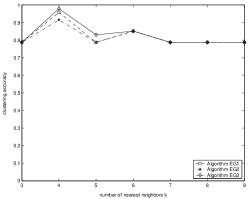
(a) Soybean dataset

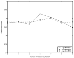
(b) Iris dataset

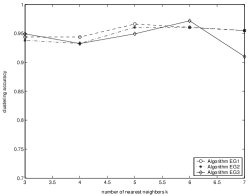
(c) Wine dataset

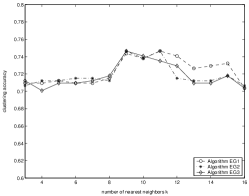
(d) Ionosphere dataset

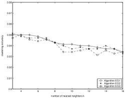
(e) Breast dataset

Figure 1: Comparison of clustering accuracies in Algorithm EG1, EG2, and EG3.

We compare our results to those results obtained by other clustering algorithms, Kmeans [32], PCA-Kmeans [32], LDA-Km [32], on the same dataset. The comparison is summarized in Table 2.

Table 2: Comparison of clustering accuracies of algorithm.

Algorithm	Soybean	Iris	Wine	Ionosphere	Breast
EG1	095.75%	090%	096.63%	074.64%	094.99%
EG2	091.49%	090.67%	096.07%	074.64%	095.14%
EG3	097.87%	090.67%	097.19%	074.64%	094.99%
Kmeans	068.1%	089.3%	070.2%	071%	0–
PCA-Kmeans	072.3%	088.7%	070.2%	071%	0–
LDA-Km	076.6%	098%	082.6%	071.2%	0–

5.2 Discussions

In the subsection, firstly, we discuss how the number of clusters is affected by the number k of nearest neighbors changing. Then, for the Algorithm EG1, the relationships between the ratio of exploration and the clustering results is investigated, which provides a way to select the ratio of exploration $\eta$. Finally, the rates of convergence in three clustering algorithms are compared.

5.2.1 Number of nearest neighbors vs. number of clusters

The number k of nearest neighbors represents the number of neighbors to which a data point $\textbf{{X}}_{i}\in\textbf{{X}}$ connects. For a dataset, the number k of nearest neighbors determines the number of clusters in part. Generally speaking, the number of clusters decreases inversely with the number k of nearest neighbors. If the number k of nearest neighbors is small, which indicates a data point $\textbf{{X}}_{i}$ connects to a few neighbors, in this case the area that the ERR function may explore is also small, i.e., the elements in the union of the extended neighbor set $\Upsilon_{t-1}(i)$ and the neighbor set $\Gamma_{t-1}(i)$ are only a few. Therefore, when the network evolves over time, strategies are spread only in a small area. Finally many small clusters with evolutionarily stable strategies appear in the network. On the other hand, a big number k of nearest neighbors provides more neighbors for a data point, which implies that the cardinality of the union is larger than that when a small k is employed. This also means that a larger area can be observed and explored by the ERR function, so that big clusters containing more data points are formed because evolutionarily stable strategies are spread in larger areas.

For a dataset, the clustering results in different number k of nearest neighbors have been illustrated in Fig. 2, in which each data point only connects to the neighbor with the largest preference, and clusters are represented by different signs. As is shown in Fig. 2, we can find that only a few data points receive considerable connections, whereas most of data points have only one connection. This indicates that when the evolution of network is ended, the network formed is characterized by the scale-free network [33], i.e., winner takes all. Besides, in Fig. 2(a), six clusters are obtained by the clustering algorithm, when $k=8$. As the number k of nearest neighbors rises, five clusters are obtained when $k=10$, three clusters when $k=15$. So, if the exact number of clusters is not known in advance, different number of clusters may be achieved by adjusting the number of nearest neighbors in practice.

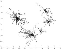
(a) $k=8$

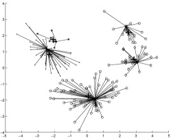
(b) $k=10$

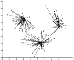
(c) $k=15$

Figure 2: The number of nearest neighbors vs. number of clusters.

5.2.2 Effect of the ratio of exploration in Algorithm EG1

For the ERR function $B^{1}_{i}(\cdot)$ used in Algorithm EG1, its capacity of exploration may be adjusted by setting different ratio of exploration $\eta\in[0,1]$. If the ratio of exploration is $\eta=0$, then the extended neighbor set formed will be empty. Hence, the network does not evolve over time, since the ERR function does not explore. On the other hand, when the ratio of exploration takes the maximum $\eta=1$, the ERR function is with the strongest capacity of exploration, because an extended neighbor set formed by all neighbors can be observed. Then we may ask naturally: what should the ratio of exploration be taken? To answer this question, we compare those clustering results at different $\eta$ shown in Fig. 3, in which the results are represented by the clustering accuracies.

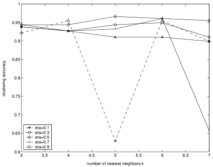
Figure 3: The results of algorithm EG1 at different rates of exploration.

From Fig. 3, we can see that when the ratio of exploration is greater than 0.5, the clustering results obtained by Algorithms EG1 fluctuates strongly, as seems over exploration. On the contrary, in the case when $\eta\leq 0.5$, the clustering results are stable relatively. As a whole, when the ratio of exploration $\eta=0.5$, the best results are achieved in Algorithm EG1. In conclusion, a big ratio of exploration is not too good, because it may cause the ERR function $B^{1}_{i}(\cdot)$ over exploration. However, if the ratio of exploration is too small, good results are not obtained because of a lack of exploration. Therefore, in the later discussion, the ratio of exploration in Algorithm EG1 takes $\eta=0.5$.

5.2.3 Three ERR functions vs. rate of convergence

As for Algorithm EG1, when $\eta=0.5$, the ERR function $B^{1}_{i}(\cdot)$ may observe the extended neighbor set formed by half of neighbors. In this case, the payoff threshold is $\theta_{t-1}^{1}(i)=median(\{u_{t-1}(j),j\in\Gamma_{t-1}(i)\})$. In Algorithm EG2, however, the ERR function $B^{2}_{i}(\cdot)$ only can observe the extended neighbor set formed by neighbors whose payoffs are greater than the average $\theta_{t-1}^{2}(i)$. Generally speaking, for the same k, the median of payoffs is smaller than or equal to the mean, i.e., $\theta_{t-1}^{1}(i)\leq\theta_{t-1}^{2}(i)$. So the exploring area of the ERR function $B^{1}_{i}(\cdot)$ is larger than that of the ERR function $B^{2}_{i}(\cdot)$, that is, the number of edges rewired in Algorithm EG1 is more than that in Algorithm EG2. In addition, the number of edges rewired in Algorithm EG3 is largest, since in Algorithm EG3 the ERR function $B^{3}_{i}(\cdot)$ provides stronger capacity of exploration for players with small payoffs, which makes more edges are removed and rewired. The comparison of number of edges rewired in three algorithms is illustrated in Fig. 4. As is shown in Fig. 4, at different number of nearest neighbors, the number of edges rewired in Algorithm EG3 is larger than that in other two, and the number of edges rewired in Algorithm EG1 is larger than Algorithm EG2. For each one of three algorithms, the number of edges rewired increases rapidly with the number of nearest neighbors.

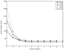
(a) EG1

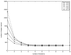
(b) EG2

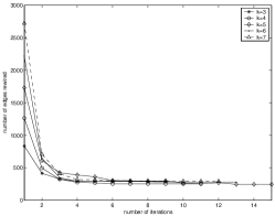
(c) EG3

Figure 4: The number of edges rewired or rates of convergence of three algorithms.

Besides, the number of iterations indicates the rate of convergence of an algorithm. From Fig. 4, we can see that the rates of convergence in Algorithm EG1 and EG2 are almost the same, and the rate of Algorithm EG3 is slower slightly than the other two because the ERR function $B^{3}_{i}(\cdot)$ in Algorithm EG3 explores larger areas than that in Algorithm EG1 and EG2. For each one of three algorithms, as the number of nearest neighbors rises, the number of iterations also rises slightly.

When the algorithm converges, the evolutionarily stable strategies appear in the network at the same time. The changes of the strategies with the largest preference for each data point are shown in Fig. 5, where the straight lines in the right side of figures represent the evolutionarily stable strategies, and the number of straight lines is the number of clusters. As is shown in Fig. 5, the evolutionarily stable strategies appear in the network after only a few iterations, as indicates the rates of convergence of algorithms are fast enough.

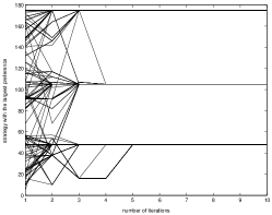
(a) EG1

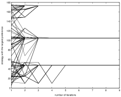
(b) EG2

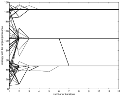
(c) EG3

Figure 5: Evolutions of strategies with the largest preference and evolutionarily stable strategies.

6 Conclusion

A model based upon games on an evolving network has been established, which may be used to explain the formation of groups in society partly. Following this model, three clustering algorithms (EG1, EG2 and EG3) using three different ERR functions are constructed, in which each data point in a dataset is regarded as a player in a game. When a distance function is selected, the initial network is created among data points according to Definition 1. Then, by applying an ERR function, the network will evolve over time due to edges removed and rewired. Hence, the preference set of a player needs to be adjusted in terms of Definition 5, and payoffs of players are recomputed too. During the network evolving, certain strategies are spread in the network. Finally, the evolutionarily stable strategies emerge in the network. According to evolutionarily stable strategies played by players, those data points with the same evolutionarily stable strategies are collected as a cluster. As such, the clustering results are obtained, where the number of evolutionarily stable strategies corresponds to the number of clusters.

The ERR functions ($B^{1}_{i}(\cdot),B^{2}_{i}(\cdot),B^{3}_{i}(\cdot)$) employed in three clustering algorithms provide different capacities of exploration for these clustering algorithms, i.e., the sizes of areas which they can observe are various. So, the clustering results of three algorithms are different. For the ERR function $B^{1}_{i}(\cdot)$, it is with a constant ratio of exploration $\eta=0.5$ because over exploration may occur when $\eta>0.5$, and can observe an extend neighbor set formed by half of neighbors. The ERR function $B^{2}_{i}(\cdot)$, however, can observe an extend neighbor set formed by neighbors whose payoffs are larger than the average, while the ERR function $B^{3}_{i}(\cdot)$ provides stronger capacity of exploration for data points with small payoffs. Besides, the clustering results of Algorithm EG1 and EG2 are more stable than that of Algorithm EG3, but the best results are achieved by Algorithm EG3 due to the strongest capacity of exploration among three algorithms.

In the case when the exact number of clusters is unknown in advance, one can adjust the number k of nearest neighbors to control the number of clusters, where the number of clusters decreases inversely with the number k of nearest neighbors. We evaluate the clustering algorithms on five real datasets, experimental results have demonstrated that data points in a dataset are clustered reasonably and efficiently, and the rates of convergence of three algorithms are fast enough.

References

- [1] J. MacQueen, Some methods for classification and analysis of multivariate observations, in: Proceedings of Fifth Berkeley Symposium on Mathematical Statistics and Probability, Vol. 1, Statistical Laboratory of the University of California, Berkeley, 1967, pp. 281–297.
- [2] J. R. Quinlan, C4.5: programs for machine learning, Morgan Kaufmann Publishers Inc., San Francisco, CA, USA, 1993.
- [3] A. Ben-Hur, D. Horn, H. T. Siegelmann, V. Vapnik, Support vector clustering, Journal of Machine Learning Research (2) (2001) 125–137.
- [4] A. Y. Ng, M. I. Jordan, Y. Weiss, On spectral clustering: Analysis and an algorithm, in: Advances in Neural Information Processing Systems 14, MIT Press, 2002, pp. 849–856.
- [5] M. B. H. Rhouma, H. Frigui, Self-organization of pulse-coupled oscillators with application to clustering, IEEE Trans. Pattern Anal. Mach. Intell. 23 (2) (2001) 180–195.
- [6] G. Folino, G. Spezzano, An adaptive flocking algorithm for spatial clustering, in: Parallel Problem Solving from Nature PPSN VII, 2002, pp. 924–933.
- [7] D. W. van der Merwe, A. P. Engelbrecht, Data clustering using particle swarm optimization, in: A. P. Engelbrecht (Ed.), Proceedings of IEEE Congress on Evolutionary Computation (CEC2003), Vol. 1, Canberra, Australia, 2003, pp. 215–220.
- [8] N. Labroche, N. Monmarché, G. Venturini, Antclust: Ant clustering and web usage mining, in: Genetic and Evolutionary Computation GECCO 2003, Vol. 2723, Chicago, IL, USA, 2003, pp. 201–201.
- [9] X. Cui, J. Gao, T. E. Potok, A flocking based algorithm for document clustering analysis, Journal of Systems Architecture 52 (8-9) (2006) 505–515.
- [10] J. v. Neumann, O. Morgenstern, Theory of Games and Economic Behavior, Princeton University Press, Princeton, New Jersey, 1944.
- [11] J. Nash, Equilibrium points in n-person games, Proceedings of the National Academy of Sciences 36 (1950) 48–49.
- [12] J. Nash, Non-cooperative games, The Annals of Mathematics 54 (2) (1951) 286–295.
- [13] J. M. Smith, Evolution and the theory of games, American Scientist 64 (1) (1976) 41–45.
- [14] J. M. Smith, G. R. Price, The logic of animal conflict, Nature 246 (5427) (1973) 15–18.
- [15] P. Pettit, R. Sugden, The backward induction paradox, The Journal of Philosophy 86 (4) (1989) 169–182.
- [16] H. A. Simon, Models of My Life, The MIT Press, Cambridge, 1996.
- [17] G. Szabó, G. Fath, Evolutionary games on graphs, Physics Reports-Review Section of Physics Letters 446 (4-6) (2007) 97–216.
- [18] J. W. Weibull, Evolutionary Game Theory, The MIT Press, Cambridge, 1995.
- [19] M. Broom, C. Cannings, G. Vickers, Evolution in knockout conflicts: The fixed strategy case, Bulletin of Mathematical Biology 62 (3) (2000) 451–466.
- [20] J. Hofbauer, K. Sigmund, Evolutionary Games and Population Dynamics, Cambridge University Press, Cambridge, 1998.
- [21] R. Axelrod, W. D. Hamilton, The evolution of cooperation, Science 211 (4489) (1981) 1390–1396.
- [22] M. A. Nowak, R. M. May, The spatial dilemmas of evolution, International Journal of Bifurcation and Chaos 3 (1) (1993) 35–78.
- [23] G. Szabó, C. Toke, Evolutionary prisoner’s dilemma game on a square lattice, Physical Review E 58 (1) (1998) 69–73.
- [24] M. Perc, A. Szolnoki, Social diversity and promotion of cooperation in the spatial prisoner’s dilemma game, Physical Review E (Statistical, Nonlinear, and Soft Matter Physics) 77 (1) (2008) 011904.
- [25] J. Vukov, G. Szabó, Evolutionary prisoner’s dilemma game on hierarchical lattices, Physical Review E (Statistical, Nonlinear, and Soft Matter Physics) 71 (3) (2005) 036133.
- [26] M. Doebeli, C. Hauert, Models of cooperation based on the prisoner’s dilemma and the snowdrift game, Ecology Letter 8 (7) (2005) 748–766.
- [27] M. A. Nowak, Five rules for the evolution of cooperation, Science 314 (5805) (2006) 1560–1563.
- [28] L. K. Grover, Quantum mechanics helps in searching for a needle in a haystack, Physical Review Letters 79 (2) (1997) 325.
- [29] M. A. Nielsen, I. L. Chuang, Quantum Computation and Quantum Information, Cambridge University Press, Cambridge, 2000.
- [30] C. Blake, C. Merz, UCI Repository of machine learning databases, Department of ICS, University of California, Irvine., http://archive.ics.uci.edu/ml/, 1998.
- [31] G. Erkan, Language model-based document clustering using random walks, in: Proceedings of the main conference on Human Language Technology Conference of the North American Chapter of the Association of Computational Linguistics, Association for Computational Linguistics, New York, New York, 2006.
- [32] C. Ding, T. Li, Adaptive dimension reduction using discriminant analysis and k-means clustering, in: Proceedings of the 24th International Conference on Machine Learning, Corvallis, OR, 2007, pp. 521–528.
- [33] A.-L. Barabási, E. Bonabeau, Scale-free networks, Scientific American 288 (5) (2003) 60–69.