Thresholding-based Iterative Selection Procedures for Model Selection and Shrinkage

Abstract

This paper discusses a class of thresholding-based iterative selection procedures (TISP) for model selection and shrinkage. People have long before noticed the weakness of the convex $l_{1}$-constraint (or the soft-thresholding) in wavelets and have designed many different forms of nonconvex penalties to increase model sparsity and accuracy. But for a nonorthogonal regression matrix, there is great difficulty in both investigating the performance in theory and solving the problem in computation. TISP provides a simple and efficient way to tackle this so that we successfully borrow the rich results in the orthogonal design to solve the nonconvex penalized regression for a general design matrix. Our starting point is, however, thresholding rules rather than penalty functions. Indeed, there is a universal connection between them. But a drawback of the latter is its non-unique form, and our approach greatly facilitates the computation and the analysis. In fact, we are able to build the convergence theorem and explore theoretical properties of the selection and estimation via TISP nonasymptotically. More importantly, a novel Hybrid-TISP is proposed based on hard-thresholding and ridge-thresholding. It provides a fusion between the $l_{0}$-penalty and the $l_{2}$-penalty, and adaptively achieves the right balance between shrinkage and selection in statistical modeling. In practice, Hybrid-TISP shows superior performance in test-error and is parsimonious.

1 Introduction

Lasso [30] has attracted people’s a lot of attention recently because it provides an efficient and continuous way for variable selection, thereby achieving a stable sparse solution. Although in the orthonormal case it is well understood and has elegant theories [12, 3, 7], its shrinking and thresholding are not direct for a general regression matrix, and it suffers some problems in both selection and estimation [39, 8, 37]. There has been a large and rapidly growing body of literature for the lasso studies over the past few years. The efficient procedures proposed for solving the lasso include the well known LARS (Efron et al. [13]), the homotopy method (Osborne et al. [26]), and a recently re-discovered iterative algorithm (Fu [17] Daubechies et al., Friedman et al. [16], Wu & Lange [33]). As for the theoretical aspects of the lasso, we refer to Knight & Fu [23], Zhao & Yu [37], Donoho et al. [11], Bunea et al. [5], Zhang & Huang [35], etc. for asymptotic and nonasymptotic results. Various extensions and modifications to lasso have also been proposed, such as the grouped lasso (Yuan & Lin [34]), the Dantzig selector (Candès and Tao [9]), the adaptive lasso (Zou [38]), and the relaxed lasso (Meinshausen & Yu [25]).

This paper aims to improve the naïve $l_{1}$-penalty, by using nonconvex penalties, to achieve an effective and efficient procedure for model selection and shrinkage. The rest of the paper is organized as follows. Section 2 provides a mechanism to borrow the rich nonconvex penalties in the orthogonal design to solve the general problem. From the point of view of thresholding rules, Section 3 constructs the thresholding-based iterative selection procedures (TISP) for model selection and successfully builds the convergence theorem. Section 4 investigates the theoretical properties of the selection and the estimation via TISPs nonasymptotically. In Section 5, we carry out an empirical study of TISP design which leads us to a novel Hybrid-TISP proposed based on hard-thresholding and ridge-thresholding. It provides a fusion between the $l_{0}$-penalty and the $l_{2}$-penalty, and adaptively achieves the right balance between shrinkage and selection in statistical modeling. In practice, Hybrid-TISP shows superior performance in both test-error and sparsity. Section 6 gives a real data example. All technical details are left to the Appendices.

2 Motivation – From Orthogonal Designs to Non-orthogonal Designs

We consider the penalized regression problem

$$\min_{\boldsymbol{\beta}}\frac{1}{2}\|{\boldsymbol{X}}{\boldsymbol{\beta}}-{\boldsymbol{y}}\|_{2}^{2}+P({\boldsymbol{\beta}};\lambda)(\triangleq f({\boldsymbol{\beta}})),$$ (2.1)

where ${\boldsymbol{X}}=\left[{\boldsymbol{x}}_{1},{\boldsymbol{x}}_{2},\cdots,{\boldsymbol{x}}_{p}\right]$ is the regression matrix, ${\boldsymbol{y}}\in R^{n}$ is the response vector, and $P({\boldsymbol{\beta}};\lambda)$ represents the penalty with $\lambda$ as the regularization parameter. Here $p$ may be greater than $n$. In this paper, we assume ${\boldsymbol{\beta}}$ is sparse, and use (2.1) for predictive learning. Although predictor error or accuracy is our first concern, we prefer to obtain a parsimonious model that is more interpretative in practice and is consistent with Occam’s razor. Usually $P$ is assumed to be an additive penalty in the sense that $P({\boldsymbol{\beta}};\lambda)$ is obtained by a univariate $P$: $P({\boldsymbol{\beta}};\lambda)=\sum P(\beta_{i};\lambda)$. This sparsity problem has wide applications in variable selection, functional data analysis, graphical modeling, compressed sensing, and so on.

If $P({\boldsymbol{\beta}};\lambda)=\lambda\|{\boldsymbol{\beta}}\|_{1}$, then (2.1) is the lasso [30], a basic and popular method in variable selection. However, although the $l_{1}$-norm provides the best convex approximation to the $l_{0}$-norm and is computationally efficient, the lasso cannot handle collinearity [39] and may result in inconsistent selection (cf. the irrepresentable conditions [37]) and introduce extra bias in estimation [25].

On the other hand, if we concentrate on orthogonal designs only, i.e., ${\boldsymbol{X}}^{T}{\boldsymbol{X}}={\boldsymbol{I}}$, like in wavelets, $l_{1}$ is far from the only choice. There are established theories and algorithms for various types of (nonconvex) penalties.

Example 1. Hard-penalties.

1. $P(\theta;\lambda)=\begin{cases}-\theta^{2}/2+\lambda|\theta|,\mbox{ if }|\theta|<\lambda\\ \lambda^{2}/2,\mbox{ if }|\theta|\geq\lambda\end{cases}$, due to Antoniadis [1].

2. $P(\theta;\lambda)=\lambda^{2}/2\cdot I_{\theta\neq 0}$, which is in fact the $l_{0}$-penalty.

3. $P(\theta;\lambda)=\begin{cases}\lambda|\theta|,\mbox{ if }|\theta|<\lambda\\ \lambda^{2}/2,\mbox{ if }|\theta|\geq\lambda\end{cases}$, due to Fan [14].

It is interesting to note that all three lead to the same estimator obtained by hard-thresholding.

Example 2. SCAD-penalty. ${P^{\prime}}(\theta;\lambda)=\begin{cases}\lambda,\mbox{ if }\theta\leq\lambda\\ (a\lambda-\theta)/(a-1),\mbox{ if }\lambda<\theta\leq a\lambda\\ 0,\mbox{ if }\theta>a\lambda\end{cases}$
for $\theta>0$ and $a>2$. The default choice of $a$ is $3.7$, based on a Bayesian argument (Fan [3]).

Example 3. Transformed $l_{1}$-penalty. $P(\theta;\lambda)={\lambda b|\theta|}/{(1+b|\theta|)}$ for some $b>0$, due to Geman & Reynolds [20].

In this simplified setup, (a) the fitting part of the penalized regression (2.1) is separable in this case, which means we only need to deal with the univariate case, if $P$ is also separable (which is true in general); (b) even if $P$ is nonconvex, it still often results in a unique solution.

One of our main goals in this paper is to borrow these rich results in the orthogonal design to help us solve the general problem (2.1). We use the following mechanism to achieve this. Define

$$g({\boldsymbol{\beta}},{\boldsymbol{\gamma}})=\frac{1}{2}\|{\boldsymbol{X}}{\boldsymbol{\gamma}}-{\boldsymbol{y}}\|_{2}^{2}+P({\boldsymbol{\gamma}};\lambda)+\frac{1}{2}<({\boldsymbol{I}}-{\boldsymbol{\Sigma}})({\boldsymbol{\gamma}}-{\boldsymbol{\beta}}),{\boldsymbol{\gamma}}-{\boldsymbol{\beta}}>.$$ (2.2)

Here $<\boldsymbol{a},\boldsymbol{b}>=\boldsymbol{a}^{T}\boldsymbol{b}$, ${\boldsymbol{\Sigma}}={\boldsymbol{X}}^{T}{\boldsymbol{X}}$.

Given ${\boldsymbol{\beta}}$, minimizing $g$ over ${\boldsymbol{\gamma}}$ is equivalent to

$$\arg\min_{\boldsymbol{\gamma}}\frac{1}{2}\left\|{\boldsymbol{\gamma}}-\left[({\boldsymbol{I}}-{\boldsymbol{\Sigma}}){\boldsymbol{\beta}}+{\boldsymbol{X}}^{T}{\boldsymbol{y}}\right]\right\|_{2}^{2}+P({\boldsymbol{\gamma}};\lambda).$$ (2.3)

In contrast to (2.1), this problem has an orthogonal design — as mentioned earlier this is easier to handle both in computation and in theory. For example, we may adopt some nonconvex penalties, and they still result in a unique solution of ${\boldsymbol{\gamma}}$.

Given ${\boldsymbol{\gamma}}$, minimizing $g$ over ${\boldsymbol{\beta}}$ is equivalent to

$$\arg\min_{\boldsymbol{\beta}}\frac{1}{2}<({\boldsymbol{I}}-{\boldsymbol{\Sigma}}){\boldsymbol{\beta}},{\boldsymbol{\beta}}-2{\boldsymbol{\gamma}}>.$$ (2.4)

Taking its derivative with respect to ${\boldsymbol{\beta}}$ gives $({\boldsymbol{I}}-{\boldsymbol{\Sigma}})({\boldsymbol{\beta}}-{\boldsymbol{\gamma}})=\boldsymbol{0}$, from which it follows that ${\boldsymbol{\beta}}={\boldsymbol{\gamma}}$ if $\|{\boldsymbol{\Sigma}}\|_{2}<1$. Note that (2.4) is a convex optimization. Therefore, the optimal value of $g$ is always achieved at ${\boldsymbol{\gamma}}={\boldsymbol{\beta}}$ if ${\boldsymbol{X}}$ is scaled down properly.

The connection to the original problem is now clear: it is easy to verify $\min_{\boldsymbol{\beta}}g({\boldsymbol{\beta}},{\boldsymbol{\beta}})$ is equivalent to $\min_{\boldsymbol{\beta}}f({\boldsymbol{\beta}})$. The advantage of optimizing $g$ instead of $f$ is that given ${\boldsymbol{\beta}}$, the problem is orthogonal and separable in ${\boldsymbol{\gamma}}$, and we can adopt far more flexible penalties in the algorithm design, including the nonconvex ones.

3 Thresholding-based Iterative Selection Procedures (TISP)

3.1 Thresholding Rules and Penalties

As the title suggests, our starting point in this paper is thresholding rules rather than different forms of the penalty function. One direct reason is that different $P$’s may result in the same estimator and the same thresholding, say, in the situation of hard-thresholding [1, 14]. Moreover, starting with thresholding functions facilitates the computation (as will be shown in the next subsection). Besides, there is also a universal connection between thresholding rules and penalty functions that we will investigate in this subsection. For convenience, we consider the univariate case only.

A thresholding function, denoted by $\Theta(\cdot;\lambda)$, with $\lambda$ as a parameter, is required to satisfy:

1. $\Theta(\cdot;\lambda)$ is an odd function. ($\Theta_{+}(\cdot;\lambda)$ is used to denote the $\Theta(\cdot;\lambda)$ restricted to $R_{+}=[0,\infty)$.)

2. $\Theta$ is a shrinkage rule: $0\leq\Theta_{+}(t;\lambda)\leq t,\forall t\in R_{+}$.

3. $\Theta_{+}$ is nondecreasing on $R_{+}$, and $\Theta_{+}(t;\lambda)\rightarrow\infty$ as $t\rightarrow\infty$.

In addition, it is natural to have $\Theta_{+}(t;\lambda)=0,0\leq t\leq\tau$ for some $\tau\geq 0$.

Given a thresholding rule $\Theta(\cdot;\lambda)$, a penalty function can be obtained from the following three-step construction. First, define

$$\Theta^{-1}(u;\lambda)=\sup\{t:\Theta(t;\lambda)\leq u\}\mbox{ and }\Theta^{-1}(-u;\lambda)=-\Theta^{-1}(u;\lambda),$$

for any $u\in R_{+}$. Then define

$$s(u;\lambda)\triangleq\Theta^{-1}(u;\lambda)-u,\forall u.$$ (3.1)

Finally, let $P$ be a continuous and positive penalty defined by

$$P(\theta;\lambda)=\int_{0}^{|\theta|}s(u;\lambda)du.$$ (3.2)

Antoniadis [2] showed the following result for this constructed $P$.

Proposition 3.1.

The minimization problem $\min_{\theta}(t-\theta)^{2}/2+P(\theta;\lambda)$ has a unique optimal solution $\hat{\theta}=\Theta(t;\lambda)$ for every $t$ at which $\Theta(\cdot;\lambda)$ is continuous.

In addition, if we define $\psi(t)=t-\Theta(t),$ then it is the psi-function for defining M-estimators; see [2, 18].

Note that (3.2) is not the only way to construct a penalty that leads to $\Theta$ in solving the optimization. For example, in the situation of hard-thresholding, in addition to the continuous penalty

$$P=\lambda^{2}/2-(|\theta|-\lambda)^{2}1_{|\theta|<\lambda}/2$$ (3.3)

constructed via (3.2),

$$P(\theta;\lambda)=\begin{cases}\lambda|\theta|,\mbox{ if }|\theta|<\lambda\\ \lambda^{2}/2,\mbox{ if }|\theta|\geq\lambda\end{cases},\mbox{ and }P(\theta;\lambda)=\frac{\lambda^{2}}{2}\cdot 1_{\theta\neq 0}$$ (3.4)

are also valid choices [1, 14]. In some sense, (3.3) may be considered as a continuous version of the discrete $l_{0}$-penalty.

3.2 TISP and Its Convergence

Now we go back to the mechanism introduced in Section 2 for the penalized multivariate regression problem (2.1), with $P$ constructed from a given thresholding function $\Theta$. Solving (2.3) yields ${\boldsymbol{\gamma}}=\Theta(({\boldsymbol{I}}-{\boldsymbol{\Sigma}}){\boldsymbol{\beta}}+{\boldsymbol{X}}^{T}{\boldsymbol{y}};\lambda)$. Seen from (2.4), our iterates simplify to

$${\boldsymbol{\beta}}^{(j+1)}=\Theta(({\boldsymbol{I}}-{\boldsymbol{\Sigma}}){\boldsymbol{\beta}}^{(j)}+{\boldsymbol{X}}^{T}{\boldsymbol{y}};\lambda).$$ (3.5)

This iterative procedure is referred to as the Thresholding-based Iterative Selection Procedure (TISP). TISP provides a feasible way to tackle the original optimization (2.1). It is a simple procedure that does not involve any complicated operations like matrix inversion.

There are rich examples for the procedure defined by (3.5). (a) Using a soft-thresholding in (3.5), we immediately obtain the iterative algorithm (in vector form) for solving the lasso problem where $P({\boldsymbol{\beta}};\lambda)=\lambda\|{\boldsymbol{\beta}}\|_{1}$ [10]. In fact, the asynchronous updating of (3.5) leads exactly to the component-by-component iteration referred to as the coordinate decent algorithm (see Friedman et al. [16]). The corresponding pathwise algorithm has been considered to be the fastest in solving the lasso problem to date, especially when $p>n$. (b) If we substitute hard-thresholding for $\Theta$, seen from (3.4), it is an alterative optimization for solving the penalized regression with

$$P=c\cdot\sum_{i}1_{\beta_{i}\neq 0}=c\cdot\|{\boldsymbol{\beta}}\|_{0},$$

i.e., the $l_{0}$-penalized regression problem. (c) We can also replace the hard-thresholding by the more smoothed SCAD to reduce instability. (d) Finally, it is worth mentioning that TISP may also include the ridge penalty $P({\boldsymbol{\beta}};\lambda)=\lambda\|{\boldsymbol{\beta}}\|_{2}^{2}/2$, if we set

$$\Theta(t;\lambda)=\frac{t}{1+\lambda},$$ (3.6)

thanks to the generic definition of a thresholding function.

Obviously, if ${\boldsymbol{\Sigma}}$ is nonsingular, and so $n>p$, the TISP mapping is a contraction and thus the sequence ${\boldsymbol{\beta}}^{(j)}$ converges to a stationary point of (2.1). We would like to apply TISP to large $p$ problems as well where ${\boldsymbol{\Sigma}}$ is singular — a surprising fact is, however, that TISP may not be a nonexpansive operator for most thresholdings (except soft-thresholding), let alone a contraction. The following studies cover the large $p$ case ($p>n$). We use $\mu(\boldsymbol{A})$ to represent an arbitrary singular value of matrix $\boldsymbol{A}$, and $\mu_{\max}(\boldsymbol{A})$ ($\mu_{\min}(\boldsymbol{A})$) the max (min) of $\mu(\boldsymbol{A})$, respectively.

Without loss of generality, suppose the penalty function defined by (3.2) satisfies the bounded curvature condition (BCC) for some symmetric matrix ${\boldsymbol{H}}$:

$$P({\boldsymbol{\beta}}+\boldsymbol{\Delta};\lambda)\geq P({\boldsymbol{\beta}};\lambda)+<\boldsymbol{\Delta},\boldsymbol{s}>-\frac{1}{2}\boldsymbol{\Delta}^{T}{\boldsymbol{H}}\boldsymbol{\Delta},\forall\boldsymbol{\Delta}\in R^{p}$$ (3.7)

where $\boldsymbol{s}=\boldsymbol{s}({\boldsymbol{\beta}};\lambda)$ is given by (3.1). Many thresholding rules of practical interest including Example 1-3 satisfy the BCC with a positive semi-definite ${\boldsymbol{H}}$. For instance, for soft-thresholding, ${\boldsymbol{H}}=\boldsymbol{0}$ since $\|{\boldsymbol{\beta}}\|_{1}$ is convex; for hard-thresholding, $\boldsymbol{H}=\boldsymbol{I}$; for SCAD-thresholding, we can take ${\boldsymbol{H}}={\boldsymbol{I}}/(a-1)$ (recall that the parameter $a$ is assumed to be greater than $2$ in Example 2, and so ${\boldsymbol{H}}$ is positive definite).

Theorem 3.1.

Given the TISP (3.5), if $\mu_{\max}({\boldsymbol{\Sigma}})\leq 1\vee(2-\mu_{\max}({\boldsymbol{H}}))$, then

$$f({\boldsymbol{\beta}}^{(j)})\geq f({\boldsymbol{\beta}}^{(j+1)}).$$ (3.8)

Moreover, if $\mu_{\max}({\boldsymbol{\Sigma}})<1\vee(2-\mu_{\max}({\boldsymbol{H}}))$, there exists a constant $C>0$, dependent on ${\boldsymbol{X}}$, ${\boldsymbol{H}}$ only, such that

$$f({\boldsymbol{\beta}}^{(j)})-f({\boldsymbol{\beta}}^{(j+1)})\geq C\cdot\|{\boldsymbol{\beta}}^{(j)}-{\boldsymbol{\beta}}^{(j+1)}\|_{2}^{2}.$$ (3.9)

Therefore, for an arbitrary ${\boldsymbol{X}}$, we can use TISP of the following form in practice

$${\boldsymbol{\beta}}^{(j+1)}=\Theta\left(\left({\boldsymbol{I}}-\frac{1}{k_{0}^{2}}{\boldsymbol{\Sigma}}\right){\boldsymbol{\beta}}^{(j)}+\frac{1}{k_{0}^{2}}{\boldsymbol{X}}^{T}{\boldsymbol{y}};\frac{\lambda}{k_{0}^{2}}\right),$$ (3.10)

where $k_{0}=\mu_{\max}({\boldsymbol{X}})=\|{\boldsymbol{X}}\|_{2}$, although larger values of $k_{0}$ generally lead to faster convergence. Applying Theorem 3.1 to some interesting special cases gives the following corollaries.

Corollary 3.1.

Suppose $\Theta$ is soft-thresholding. If $\mu_{\max}({\boldsymbol{X}})<\sqrt{2}$, then (3.9) holds.

Corollary 3.2.

Suppose $\Theta$ is hard-thresholding. If $\mu_{\max}({\boldsymbol{X}})\leq 1$, then (3.8) holds; further, if $\mu_{\max}({\boldsymbol{X}})<1$, then (3.9) is true.

Corollary 3.3.

Suppose $\Theta$ is SCAD-thresholding. If $\mu_{\max}({\boldsymbol{X}})<\sqrt{2-\frac{1}{a-1}}$, then (3.9) holds.

Corollary 3.1 generalizes the lasso result by Daubechies et al. [10], and coincides with our previous study [27]. Corollary 3.3 covers the orthogonal case, since SCAD assumes $a>2$ and thus $\sqrt{2-\frac{1}{a-1}}>1$. Finally, it is worth pointing out that TISP may not always be an MM algorithm [21] like the LLA method by Zou & Li [40]. Take the SCAD-thresholding as an example: when $1<\|{\boldsymbol{X}}\|_{2}<\sqrt{2-\frac{1}{a-1}}$, $g$ defined by (2.2) does not majorize $f$ but TISP converges. Theorem 3.1 implies that if ${\boldsymbol{X}}$ is scaled down properly (which does not affect the variable selection), $f({\boldsymbol{\beta}}^{(j)})$ is nonincreasing all the time during the iteration process.

We can easily show a result similar to Zou & Li [40]:

Proposition 3.2.

Suppose $\mu_{\max}({\boldsymbol{\Sigma}})<1\vee(2-\mu_{\max}({\boldsymbol{H}}))$. Give an initial point ${\boldsymbol{\beta}}{(0)}$, if ${\boldsymbol{\beta}}^{*}$ is a limit point of the TISP sequence ${\boldsymbol{\beta}}^{(j)}$, then ${\boldsymbol{\beta}}^{*}$ is a stationary point of $f({\boldsymbol{\beta}})$ (2.1), or equivalently, a fixed point of (3.5).

Denote by $F$ the set of the fixed points of TISP. That is, given any ${\boldsymbol{\beta}}^{*}\in F$, it satisfies the implicit equation

$${\boldsymbol{\beta}}=\Theta(({\boldsymbol{I}}-{\boldsymbol{\Sigma}}){\boldsymbol{\beta}}+{\boldsymbol{X}}^{T}{\boldsymbol{y}};\lambda),$$ (3.11)

referred to as the $\Theta$-equation. Clearly, local minima of $f$ are fixed points of (3.11). In the next section, we will perform an nonasymptotic study of the good properties of the points in $F$. Here, we give the following optimality result.

Proposition 3.3.

Let ${\boldsymbol{\beta}}^{*}\in F$ and suppose $\mu_{\max}({\boldsymbol{H}})\leq 1$. If $\mu_{\max}({\boldsymbol{H}})\leq\mu({\boldsymbol{\Sigma}})\leq 2-\mu_{\max}({\boldsymbol{H}})$, then ${\boldsymbol{\beta}}^{*}$ is a global minimizer of $f$.

Although the fact that nonconvex penalties often result in a unique optimal solution in the orthogonal design is well known, this proposition states (novelly) that the same conclusion holds as long as ${\boldsymbol{X}}$ is not too far from orthogonal (characterized in terms of ${\boldsymbol{H}}$). For instance, for SCAD thresholding and penalty, TISP necessarily leads to the global minimum of $f$, provided $\frac{1}{\sqrt{a-1}}\leq\mu({\boldsymbol{X}})\leq\sqrt{2-\frac{1}{a-1}}$, or $0.61\leq\mu({\boldsymbol{X}})\leq 1.27$ when $a=3.7$ (the default choice in SCAD–see Example 2), given any initial point ${\boldsymbol{\beta}}^{(0)}$. In summary, TISP is a successful algorithm for solving the penalized regressions for a general design matrix.

3.3 Related Work

The main contribution of this paper is to consider a new class of $\Theta$-estimators defined by the $\Theta$-equation (3.11) for model selection and shrinkage, which can be naturally computed by TISP, and are associated with penalized regressions—in particular, the penalty $P$ can be constructed via the three-step procedure introduced in Section 3.1. More generally, the $\lambda$ in (3.11) can be component-specific. For example, if ${\boldsymbol{X}}$ is not column-normalized, we may use

$${\boldsymbol{\beta}}=\Theta\left(\left({\boldsymbol{I}}-{\boldsymbol{\Sigma}}\right){\boldsymbol{\beta}}+{\boldsymbol{X}}^{T}{\boldsymbol{y}};\boldsymbol{\lambda}\right),$$ (3.12)

where $\boldsymbol{\lambda}=\left[\begin{array}[]{cccc}\lambda\|{\boldsymbol{x}}_{1}\|_{2}&\lambda\|{\boldsymbol{x}}_{2}\|_{2}&\cdots&\lambda\|{\boldsymbol{x}}_{p}\|_{2}\end{array}\right]^{T}$ and $\lambda$ is a regularization parameter. With a carefully designed $\Theta$, we obtain a good estimator with both accuracy and sparsity, as will be shown in Section 5.2. The corresponding penalty is, not surprisingly, nonconvex, which indicates the difficulty of this NP-hard problem.

Nonconvex penalties have been successfully used in real-world applications like high-dimensional nonparametric modeling [3], survival analysis [6], and microarray data analysis [32, 36], where they achieve outstanding performance. The numerical optimization has been a challenging and intriguing problem. In the context of wavelet denoising where ${\boldsymbol{X}}{\boldsymbol{X}}^{T}={\boldsymbol{I}}$, Antoniadis & Fan [3] proposed the ROSE to approximately solve the minimization problem for a wide class of nonconvex penalties. They also introduced the graduated nonconvexity (GNC) algorithm, developed in image processing; it has a number of tuning parameters and is computationally intensive. Fan and Li [15] then proposed a generic local quadratic approximation (LQA) algorithm by solving a series of $l_{2}$-penalized problems. Like ridge regression, this approach does not intrinsically yield zeros, and setting a small cutoff value during iteration has been shown to be too greedy. A refined version is the perturbed LQA suggested by Hunter & Li [22] to avoid numerical instability. The perturbation parameter needs to be chosen very carefully in implementation since it affects the sparsity of the solution as well as the speed of convergence. Recently, Zou & Li [40] proposed a new local linear approximation (LLA) which significantly improves the LQA. Explicit sparsity is attained by solving a weighted lasso problem at each iteration step. (Note that our TISP does a simple thresholding at each step.) One-step SCAD estimator is advocated. Our empirical studies show that this one-step convex approximation has limited power in finite samples. Although the estimate is sparser than using the plain $l_{1}$-penalty, it may result in misleading models with poor prediction error. See Section 5 for detail.

Using thresholding rules to define $\Theta$-estimators shares similarities to the studies of $M$-estimators of $\psi$-type in robust regression. Most $M$-estimators were proposed in the form of $\psi$-functions but not based on loss functions, such as Huber’s, Hampel’s three-part, and Tukey’s bisquare $M$-estimators. Indeed, we find an interesting connection between these two fields. Assume a mean shift outlier model, ${\boldsymbol{y}}={\boldsymbol{X}}{\boldsymbol{\beta}}+{\boldsymbol{\gamma}}+{\boldsymbol{\epsilon}},{\boldsymbol{\epsilon}}\sim N(0,\sigma^{2}{\boldsymbol{I}})$, where $n>p$ and ${\boldsymbol{\gamma}}\in R^{n}$ is sparse. If ${\boldsymbol{\gamma}}_{i}$ is nonzero, case $i$ is an outlier. Let ${\boldsymbol{H}}={\boldsymbol{X}}({\boldsymbol{X}}^{T}{\boldsymbol{X}})^{-1}{\boldsymbol{X}}^{T}$ be the hat matrix and suppose its spectral decomposition is given by ${\boldsymbol{H}}={\boldsymbol{U}}{\boldsymbol{D}}{\boldsymbol{U}}^{T}$. Define an index set $c=\{i:D_{ii}=0\}$ and ${\boldsymbol{U}}_{c}$ is formed by taking the corresponding columns of ${\boldsymbol{U}}$. Then a reduced model can be obtained from the mean shift outlier model

$$\tilde{\boldsymbol{y}}={\boldsymbol{A}}{\boldsymbol{\gamma}}+{{\boldsymbol{\epsilon}}^{\prime}},{\boldsymbol{\epsilon}}^{\prime}\sim N(\boldsymbol{0},\sigma^{2}{\boldsymbol{I}}_{(n-p)\times(n-p)}),$$ (3.13)

where $\tilde{\boldsymbol{y}}={\boldsymbol{U}}_{c}^{T}{\boldsymbol{y}}$, ${\boldsymbol{A}}={\boldsymbol{U}}_{c}^{T}$ (of dimension ${(n-p)\times n}$). Applying $\Theta$-TISP to this ‘large-$p$’ sparsity problem gives the iteration ${\boldsymbol{\gamma}}^{(j+1)}=\Theta({\boldsymbol{A}}^{T}\tilde{\boldsymbol{y}}/k_{0}^{2}+({\boldsymbol{I}}-{\boldsymbol{A}}^{T}{\boldsymbol{A}}/k_{0}^{2}){\boldsymbol{\gamma}}^{(j)};\boldsymbol{\lambda}/k_{0}^{2})$ with $k_{0}=\mu_{max}({\boldsymbol{H}})$, or

$${\boldsymbol{\gamma}}^{(j+1)}=\Theta({\boldsymbol{H}}{\boldsymbol{\gamma}}^{(j)}+({\boldsymbol{I}}-{\boldsymbol{H}}){\boldsymbol{y}};\boldsymbol{\lambda}).$$

After getting $\hat{\boldsymbol{\gamma}}$ from TISP, we can estimate ${\boldsymbol{\beta}}$ by $\hat{\boldsymbol{\beta}}=({\boldsymbol{X}}^{T}{\boldsymbol{X}})^{-1}{\boldsymbol{X}}^{T}({\boldsymbol{y}}-\hat{\boldsymbol{\gamma}})$. Simple algebra shows that this special $\Theta$-TISP solves an $M$-estimation problem associated with $\psi$, if ($\Theta$, $\psi$) satisfies $\Theta(t;\lambda)+\psi(t;\lambda)=t.$ It is well known that Huber’s method (or equivalently, Soft-TISP, which corresponds to using a convex $l_{1}$-penalty on ${\boldsymbol{\gamma}}$) behaves poorly in outlier detection even for moderate leverage points. Instead, redescending $\psi$-functions are advocated, which corresponds to using nonconvex penalties for the sparsity problem of (3.13).

4 Selection and Estimation via TISP

TISP provides a very simple way to do variable selection via penalized regressions. In this section, we will perform a theoretical study of the variable selection and coefficient estimation by TISPs based on different thresholdings. Our results are nonasymptotic.

4.1 Assumptions on $\Theta$

Given $\Theta(\cdot;\lambda)$, denote its thresholding value by $\tau(\lambda)$, i.e., $\Theta(t;\lambda)=0\mbox{ }\forall t:|t|<\tau$ and $\Theta(t;\lambda)\neq 0\mbox{ for }|t|>\tau$. For example, $\tau(\lambda)=\lambda$ in soft-, hard-, and SCAD-thresholdings, but is not so for the transformed $l_{1}$. Assume $\tau>0$. To ease our TISP study based on the $\Theta$-equation (3.11), we define another version of ${\boldsymbol{s}}$, called the generalized sign. Introduce

$${\widetilde{\mbox{Sgn}}}(u;\lambda)=\{s\in R:\Theta(u+\tau s;\lambda)=u\}\quad\mbox{ if }u\in\mbox{ran}(\Theta),$$

and ${\widetilde{\mbox{Sgn}}}(u;\lambda)=\{0\}$ otherwise, where $\mbox{ran}(\Theta)$ is the range of $\Theta$; ${\widetilde{\mbox{sgn}}}(u;\lambda)$ is used to denote a specific element in ${\widetilde{\mbox{Sgn}}}(u;\lambda)$. The vector versions of ${\widetilde{\mbox{Sgn}}}$ and ${\widetilde{\mbox{sgn}}}$ can be defined correspondingly. Clearly if $u=\Theta(t;\lambda)$ then $t=u+\tau{\widetilde{\mbox{sgn}}}(u;\lambda)$ for some ${\widetilde{\mbox{sgn}}}(u;\lambda)\in{\widetilde{\mbox{Sgn}}}(u;\lambda)$.

As a demonstration, if $\Theta(\cdot;\lambda)$ is soft-thresholding, $\tau=\lambda$ and $\widetilde{\mbox{Sgn}}({\boldsymbol{\beta}})=\{\boldsymbol{s}:s_{i}=1{\mbox{ if }}\beta_{i}>0,s_{i}=-1{\mbox{ if }}\beta_{i}<0,{\mbox{ and }}s_{i}\in[-1,1]{\mbox{ if }}\beta_{i}=0\}$. Thus now ${\widetilde{\mbox{Sgn}}}({\boldsymbol{\beta}})$ is the subdifferential of $\|{\boldsymbol{\beta}}\|_{1}$, and ${\widetilde{\mbox{sgn}}}({\boldsymbol{\beta}})$ is a subgradient [29]. For hard-thresholding, $\widetilde{\mbox{Sgn}}({\boldsymbol{\beta}})=\{\boldsymbol{s}:s_{i}=0{\mbox{ if }}\beta_{i}\neq 0,s_{i}\in[-1,1]{\mbox{ if }}\beta_{i}=0\}$. $\widetilde{\mbox{Sgn}}$ and $\widetilde{\mbox{sgn}}$ are called generalized signs due to the following fact.

Proposition 4.1.

Suppose $\Theta(\cdot;\lambda)$ is sandwiched by soft- and hard-thresholdings, $\Theta_{S}(\cdot;\tau)$ and $\Theta_{H}(\cdot;\tau)$, i.e.,

$$(\Theta_{S})_{+}(t;\tau)\leq\Theta_{+}(t;\lambda)\leq(\Theta_{H})_{+}(t;\tau),\forall t\in R_{+}.$$ (4.1)

Then $0\leq{\widetilde{\mbox{sgn}}}(u)\leq 1$ if $u>0$, $-1\leq{\widetilde{\mbox{sgn}}}(u)\leq 0$ if $u<0$, and ${\widetilde{\mbox{sgn}}}(0)\in[-1,1]$.

This proposition is easy to prove from the non-decreasing property of $\Theta$. Throughout the rest of the section, we assume $\Theta$ always satisfies the sandwiching condition (4.1). By the definition of the generalized signs, (3.11) is equivalent to ${\boldsymbol{\Sigma}}{\boldsymbol{\beta}}={\boldsymbol{X}}^{T}{\boldsymbol{y}}-\tau{\widetilde{\mbox{sgn}}}({\boldsymbol{\beta}};\lambda),$ for some ${\widetilde{\mbox{sgn}}}({\boldsymbol{\beta}};\lambda)\in{\widetilde{\mbox{Sgn}}}({\boldsymbol{\beta}};\lambda)$. We study the TISP estimate based on the scaled form (3.10). Let $\hat{\boldsymbol{\beta}}$ be a fixed point of (3.10) and suppose $\tau(\lambda)=c\tau(\lambda/c)$ for any $c>0$. Then the $\Theta$-equation for this TISP estimate can be rewritten as

$${\boldsymbol{\Sigma}}\hat{\boldsymbol{\beta}}={\boldsymbol{X}}^{T}{\boldsymbol{y}}-\tau{\widetilde{\mbox{sgn}}}(\hat{\boldsymbol{\beta}};\lambda/k_{0}^{2}),$$ (4.2)

where $k_{0}=\|{\boldsymbol{X}}\|_{2}$.

4.2 Sparsity Recovery

Recall that ${\boldsymbol{y}}={\boldsymbol{X}}{\boldsymbol{\beta}}+{\boldsymbol{\epsilon}}$, ${\boldsymbol{\epsilon}}\sim N(\boldsymbol{0},\sigma^{2}\boldsymbol{I})$, and ${\boldsymbol{\beta}}$ is sparse. Let $z=\{i:\beta_{i}=0\}$, $nz=\{i:\beta_{i}\neq 0\}$, $d_{z}=|z|$, $d_{nz}=|nz|$. To study the sign-consistency of a TISP estimate, we denote by $p_{s}$ the probability of successful sign recovery, that is, the probability that there exists a $\hat{\boldsymbol{\beta}}\in F$ such that ${\mbox{sgn}}(\hat{\boldsymbol{\beta}})={\mbox{sgn}}({\boldsymbol{\beta}})$.

To simplify asymptotic discussions, we assume ${\boldsymbol{X}}$ has been scaled to have all column $l_{2}$-norms equal to $\sqrt{n}$. Define ${\boldsymbol{\Sigma}}^{(s)}={\boldsymbol{\Sigma}}/n$. To get a better form of the bounds for $p_{s}$, we define two quantities $\mu=\mu_{\min}({\boldsymbol{\Sigma}}_{nz,nz}^{(s)})$ and $\kappa\triangleq\underset{i\in z}{\max}\|{\boldsymbol{\Sigma}}_{i,nz}^{(s)}\|_{2}/\sqrt{d_{nz}}$. Intuitively, $\kappa$ measures the ‘mean’ correlations between the relevant predictors and the irrelevant predictors. The following nonasymptotic result is always true regarding the selection via TISP.

Theorem 4.1.

Assume $\mu\geq\kappa d_{nz}$, $\mu>0$ and $\min|{\boldsymbol{\beta}}_{nz}|\geq\frac{d_{nz}\tau}{n\mu}$, then

$$p_{s}\geq[1-2\Phi(-M)]^{d_{z}}[1-2\Phi(-L)]^{d_{nz}},$$ (4.3)

where $M=\left(1-\frac{\kappa d_{nz}}{\mu}\right)\frac{\tau}{\sqrt{n}\sigma}$, $L=\frac{\sqrt{\mu n}}{\sigma}\left(\min|{\boldsymbol{\beta}}_{nz}|-\frac{\tau d_{nz}}{{\mu n}}\right)$, and $\Phi$ is the standard normal distribution.

Corollary 4.1.

Under the conditions of Theorem 4.1, we have

$$1-p_{s}\leq 2d_{z}\varphi(M)/M+2d_{nz}\varphi(L)/L,$$ (4.4)

where $\varphi$ is the standard normal density.

Clearly, the size of $\kappa$ is very important. A small value of $\kappa$ weakens the interference of ${\boldsymbol{X}}_{z}$ and ${\boldsymbol{X}}_{nz}$ and helps recover the sparsity correctly. We can also use this theorem to explore some asymptotics. (i) Assume ${\boldsymbol{\beta}}$, $d_{z}$, and $d_{nz}$ are fixed, $n\rightarrow\infty$, then under some regularity conditions we get: if $\tau/\sqrt{n}\rightarrow\infty$ and $\tau/n\rightarrow 0$, then TISP is sign consistent. This result in the Soft-TISP (lasso) case coincides with other studies like [23, 37]. (ii) Suppose ${\boldsymbol{\beta}}_{nz}$ and $d_{nz}$ are fixed, $n,d_{z}\rightarrow\infty$, and $\mu\geq(1+\epsilon)\kappa d_{nz}$ for some $\epsilon>0$. Then TISP can successfully recover the sparsity pattern of ${\boldsymbol{\beta}}$ if $d_{z}\varphi(M)/M\rightarrow 0$ and $\tau/n\rightarrow 0$, which only requires $n$ to grow faster than $\log d_{z}$.

Unfortunately, the regularity condition $\mu\geq\kappa d_{nz}$ cannot be removed in general. In the lasso case, it is a version of the irrepresentable conditions [37]. (We took this more restrictive form because it is more intuitive and leads to more nice-looking bounds in (4.3) and (4.4).) However, for hard-thresholding-like $\Theta$’s, this is unnecessary and we can obtain stronger results.

We say that $\Theta$ belongs to the hard-thresholding family if

$$\Theta(t;\lambda)=t,\forall t:|t|>c\cdot\tau,$$ (4.5)

for some constant $c\geq 1$. Hard-thresholding and SCAD-thresholding are two examples with $c=1$, $a$ respectively. Unlike soft-thresholding, they do not introduce bias for large nonzero components.

Theorem 4.2.

Suppose $\Theta$ belongs to the hard-thresholding family and $\min|{\boldsymbol{\beta}}_{nz}|\geq c\tau/k_{0}^{2}$. Then

$$p_{s}\geq[1-2\Phi(-M^{\prime})]^{d_{z}}[1-2\Phi(-L^{\prime})]^{d_{nz}},$$ (4.6)

where $M^{\prime}=\frac{c\tau}{\sqrt{n}\sigma}$, $L^{\prime}=\frac{\sqrt{\mu n}}{\sigma}\left(\min|{\boldsymbol{\beta}}_{nz}|-\frac{c\tau}{k_{0}^{2}}\right)$.

Corollary 4.2.

Under the conditions of Theorem 4.2, we have

$$1-p_{s}\leq 2d_{z}\varphi(M^{\prime})/M^{\prime}+2d_{nz}\varphi(L^{\prime})/L^{\prime}.$$ (4.7)

(4.6) is strictly better than the bound in (4.3) if $c<d_{nz}k_{0}^{2}/(\mu n)$, or $c<d_{nz}{\mu_{\max}({\boldsymbol{\Sigma}}^{(s)})}/{\mu_{\min}({\boldsymbol{\Sigma}}^{(s)}_{nz})}$, which is usually true for both hard- and scad-thresholding. Therefore the TISP induced by a $\Theta$ in the hard-thresholding family can achieve better performance in variable selection. This will be verified empirically in the next section. Note that although in the orthogonal case, hard-thresholding and soft-thresholding give exactly the same zeros, they result in very different sparsity patterns in our iterative procedure for a nonorthogonal ${\boldsymbol{X}}$.

4.3 Estimation Risk

We obtain the following TISP risk bounds for any thresholding $\Theta$.

Theorem 4.3.

Let $\nu=\mu_{\min}({\boldsymbol{\Sigma}}_{z,z}^{(s)})$ and $\hat{\boldsymbol{\beta}}\in F$. Define $R_{nz}=E(\|{\boldsymbol{\beta}}_{nz}-\hat{\boldsymbol{\beta}}_{nz}\|_{2}^{2})$, and $R_{z}=E(\|\hat{\boldsymbol{\beta}}_{z}\|_{2}^{2})$. Suppose ${\boldsymbol{\Sigma}}$ is nonsingular. Then

$$R_{nz}\leq\frac{3}{n}\left[\frac{d_{nz}}{\mu}\sigma^{2}+\frac{d_{nz}}{\mu^{2}}\frac{\tau^{2}}{n}+\kappa^{2}\frac{d_{z}d_{nz}}{\mu^{2}}\cdot nR_{z}\right].$$ (4.8)

And

$$R_{z}\leq\frac{\sigma^{2}}{n}\frac{d_{z}^{2}}{\nu^{2}}(K_{1}M+K_{2}\frac{1}{M})\varphi(M),$$ (4.9)

where $M$ is defined as in Theorem 4.1, $K_{1}=6\frac{1+\frac{1+{\kappa^{2}d_{nz}^{2}}/{\mu^{2}}}{\left(1-{\kappa d_{nz}}/{\mu}\right)^{2}}}{\left(1-\kappa^{2}\frac{d_{z}d_{nz}}{\mu\nu}\right)^{2}}$, $K_{2}=6{\left(1-\kappa^{2}\frac{d_{z}d_{nz}}{\mu\nu}\right)^{-2}}$ in which we assume $\kappa^{2}\leq\frac{\mu\nu}{d_{z}d_{nz}}$ and $\mu\geq\kappa d_{nz}$.

This general result holds for any TISP estimate. It is not difficult to show that in the previous setting of (i) where ${\boldsymbol{\beta}}$ is fixed, we also obtain $R_{z}\rightarrow 0$ and $R_{nz}\rightarrow 0$ by the theorem if $\tau/\sqrt{n}\rightarrow\infty$ and $\tau/n\rightarrow\infty$. Besides, under the conditions stated in the theorem, $M=\sqrt{2\log\frac{d_{z}^{2}}{n}+(1+\epsilon)\log\log\frac{d_{z}^{2}}{n}}$ is sufficient to ensure $R_{z}\rightarrow 0$ for any $\epsilon>0$; since $M\sim\sqrt{2\log\frac{d_{z}^{2}}{n}}\leq\sqrt{2\log d_{z}}$, Donoho & Johnstone’s classical work [12] in the orthogonal design implies this risk bound can not be improved significantly in general. We leave the TISP design problem to the next section using an empirical study.

In the orthogonal case, we can show the oracle inequalities [12] hold.

Theorem 4.4.

Suppose $\Theta$ satisfies the sandwiching condition (4.1) and ${\boldsymbol{X}}^{T}{\boldsymbol{X}}={\boldsymbol{I}}$. Then

$$E\|\hat{\boldsymbol{\beta}}-{\boldsymbol{\beta}}\|_{2}^{2}\leq(1+\tau^{2})\sum_{1}^{n}\min\left(\frac{2\varphi(\tau)}{\tau}\sigma^{2}+\beta_{i}^{2},\sigma^{2}\right)$$ (4.10)

for any $\tau>1$. Consequently, when $\tau=\sqrt{2\log n}$,

$$E\|\hat{\boldsymbol{\beta}}-{\boldsymbol{\beta}}\|_{2}^{2}\leq(2\log n+1)\left(\frac{\sigma^{2}}{\sqrt{\pi\log n}}+\sum\min(\beta_{i}^{2},\sigma^{2})\right)$$ (4.11)

for any $n\geq 2$.

This nonasymptotic result covers soft-, hard-, and SCAD-thresholdings. It coincides with the classical soft-thresholding studies [12] and is sharper than [3, 38]. (A correction of Zou’s oracle bound [38] is also given at the end of the proof; see Appendix A.4.)

5 TISP Designs: An Empirical Study

5.1 A numerical study of TISPs

In this section, we demonstrate the empirical performance of TISPs by some simulation data. Although there are rich choices about $\Theta$ in (3.5), we focus on three basic TISPs only in this subsection. In addition to the Soft-TISP, i.e., the lasso, we implemented Hard-TISP and SCAD-TISP, the thresholdings of which belong to the hard-thresholding family. The parameter $a$ in SCAD-thresholding takes the default value, $3.7$, based on a Bayesian argument [15]. As seen from the theoretical studies in Section 4, the last two should perform better than the lasso in variable selection. In generating the solution path for a grid of $\lambda$-values, we always set the initial point, ${\boldsymbol{\beta}}^{(0)}$, to be zero in Hard- or SCAD-TISP. A natural search range for $\lambda$, seen from (3.11), is $[0,{\boldsymbol{X}}^{T}{\boldsymbol{y}}]$, if ${\boldsymbol{X}}$ has been column normalized. (Note that a pathwise algorithm with warm start, which takes the previous estimate associated with the old value of $\lambda$ as the initial point of the procedure for the current value of $\lambda$, may be inappropriate for TISPs when nonconvex penalties are used. In fact, the solution path associated with a nonconvex penalty is generally not continuous in $\lambda$ and warm-start leads to bad solutions because of multiple local minima effects.)

For comparison, the one-step LLA method, proposed by Zou & Li [40] for penalized likelihood models, is also included in our tests. They showed good asymptotics about one-step SCAD when $n\rightarrow\infty$ and $p$ is fixed, and demonstrated its performance in various numerical examples. The one-step LLA is actually a weighted lasso with weights constructed from the OLS estimate using different penalty functions. According to our general result of weights in sparse regression [27], it can achieve better sign consistency than the lasso as $n$ grows to infinity. We are greatly interested in drawing a comparison between TISP and LLA since TISP also successfully solves the penalized regression problems.

We did experiments on two simulation datasets. Each dataset contains training data, validation data, and test data. We use $\#=$“$\cdot/\cdot/\cdot$” to denote the number of observations in the training data, validation data, and test data. Let ${\boldsymbol{\Sigma}}$ be the correlation matrix in generating ${\boldsymbol{X}}$, i.e., each row of ${\boldsymbol{X}}$ is independently drawn from $N(\boldsymbol{0},{\boldsymbol{\Sigma}})$. We use $(\{a_{1}\}^{n_{1}},\cdots,\{a_{k}\}^{n_{k}})$ to denote the column vector made by $n_{1}$ $a_{1}$’s, $\cdots$, $n_{k}$ $a_{k}$’s consecutively in the following examples.
Example 1. $\#=20/100/200$, $d=8$, ${\boldsymbol{\beta}}=(\{3\}^{1},\{1.5\}^{1},\{0\}^{2},\{2\}^{1},\{0\}^{3})$, $\Sigma_{ij}=\rho^{|i-j|}$ with $\rho=0.5$, $\sigma=2,3,5,8$; the corresponding signal-to-noise variance ratio (${\boldsymbol{\beta}}^{T}{\boldsymbol{\Sigma}}{\boldsymbol{\beta}}/\sigma^{2}$) is $5.31$, $2.36$, $0.85$, and $0.33$, respectively.
Example 2. $\#=20/100/200$, $d=8$, ${\boldsymbol{\beta}}=(\{3\}^{1},\{1.5\}^{1},\{0\}^{2},\{2\}^{1},\{0\}^{3})$, $\Sigma_{ij}=\rho^{|i-j|}$ with $\rho=0.85$, $\sigma=2,3,5,8$; the corresponding signal-to-noise variance ratio is $8.21$, $3.65$, $1.31$, and $0.51$, respectively.
Before an algorithm is applied, the columns of a regression matrix are all normalized to have a squared $l_{2}$-norm equal to the number of the observations; no centering is performed in these examples.

Each model is simulated 50 times, then, we measure the performance of each algorithm mainly by test error and sparsity error. The test error is characterized by the $40\%$ trimmed-mean of the scaled MSE (SMSE) on the test data, where SMSE is $100\cdot(\sum_{i=1}^{N}(\hat{y}_{i}-y_{i})^{2}/(N\sigma^{2})-1)$ defined for the test data. (Medians of MSEs are mostly used [30, 39] to measure the performance from multiple runs, but are not so stable for comparisons based on our experience.) The sparsity error here is defined by the $40\%$ trimmed-mean of the following 50 percentages: $100\cdot|\{i:\mbox{sgn}(\hat{\beta}_{i})\neq\mbox{sgn}(\beta_{i})\}|/d$, which represents the number of inconsistent signs for each estimate compared to the true ${\boldsymbol{\beta}}$. We also summarized the proper zero percentages, $100\%\cdot|\{i:\beta_{i}=0,\hat{\beta}_{i}=0\}|/|\{i:\beta_{i}=0\}|$, and the proper nonzero percentages, $100\%\cdot|\{i:\beta_{i}\neq 0,\hat{\beta}_{i}\neq 0\}|/|\{i:\beta_{i}\neq 0\}|$ in the table as follows. The numbers in parentheses are the standard errors of the trimmed means of SMSE, estimated by bootstrapping the SMSE $500$ times as in [38]. The total computing time (in seconds) for each algorithm is also included.

		Lasso	One-step SCAD	Hard-TISP	SCAD-TISP	eNet	Hybrid-TISP
EX1, $\sigma=2$	Test-err	28.6(3.6)	25.3(4.9)	21.7(3.7)	18.2(3.4)	25.4(3.5)	15.9(3.4)
	Spar-err	31.8	12.5	0	12.5	31.0	0
	Prop-Z	50.8%	91.2%	100%	89.5%	51.2%	100%
	Prop-NZ	100%	100%	100%	100%	100%	100%
EX1, $\sigma=3$	Test-err	27.8(3.4)	27.4(3.5)	25.9(3.6)	25.8(3.5)	23.4(3.5)	18.2(4.0)
	Spar-err	30.7	16.7	5.5	12.5	31.5	3.8
	Prop-Z	50.8%	80.0%	93.2%	92.0%	47.3%	94.1%
	Prop-NZ	100%	87.2%	100%	100%	100.0%	100.0%
EX1, $\sigma=5$	Test-err	23.0(3.8)	27.0(2.5)	22.3(2.7)	25.7(3.1)	18.4(3.6)	17.8(3.5)
	Spar-err	32.0	25.0	12.5	25.0	31.5	12.5
	Prop-Z	50.4%	80.0%	91.6%	80.0%	48.6%	92.3%
	Prop-NZ	86.2%	66.7%	85.1%	66.7%	100.0%	100%
EX1, $\sigma=8$	Test-err	15.4(2.9)	20.4 (2.6)	20.3(2.9)	17.1(2.9)	14.1(2.8)	11.3(2.6)
	Spar-err	31.3	30.5	25.0	32.8	37.5	30.6
	Prop-Z	72.3%	80.0%	94.9%	80.0%	70.4%	94.7%
	Prop-NZ	66.7%	33.3%	49.5%	33.3%	66.7%	66.7%
EX2, $\sigma=2$	Test-err	24.1(2.1)	28.7(4.1)	19.9(2.8)	20.8(2.9)	19.4(3.5)	14.3(3.2)
	Spar-err	31.0	32.0	12.5	12.5	30.8	12.5
	Prop-Z	60.0%	74.5%	80.0%	90.5%	52.3%	80%
	Prop-NZ	100%	84.1%	100%	100%	100.0%	100.0%
EX2, $\sigma=3$	Test-err	19.9(3.3)	29.1(3.1)	19.8(2.2)	20.2(2.4)	14.3(2.9)	14.1(2.9)
	Spar-err	30.7	29.8	16.1	16.3	28.6	17.3
	Prop-Z	60.0%	80.0%	91.1%	91.9%	55.8%	80%
	Prop-NZ	85.7%	66.7%	83.7%	66.7 %	100.0%	100.0 %
EX2, $\sigma=5$	Test-err	13.9(3.1)	24.8(2.2)	16.6(2.6)	17.4(2.7)	9.7(2.6)	9.0(2.7)
	Spar-err	31.0	31.3	25.0	25.0	30.0	25
	Prop-Z	68.8%	80.0%	80.0%	80.0%	52.9%	80%
	Prop-NZ	66.7%	48.2%	66.7%	66.7%	100.0%	84.1%
EX2, $\sigma=8$	Test-err	10.4(2.6)	16.3(2.1)	13.8(2.8)	15.6(2.8)	7.2(2.2)	6.9(2.5)
	Spar-err	32.0	36.4	31.0	29.0	37.5	30.4
	Prop-Z	71.0%	80.0%	92.1%	91.0%	49.3%	74.6%
	Prop-NZ	66.7%	33.3%	47.4%	33.3%	83.0%	66.7%
Total computing time		284	599	596	610	2185	2234

Table 1: Performance comparisons on the simulation data, in terms of test error, sparsity error, proper sparsity, and proper nonsparsity – all the numbers are 40% trimmed-mean of the 50 simulations. Six methods are listed here: lasso (Soft-TISP), one-step SCAD, Hard-TISP, SCAD-TISP, elastic net (eNet), and Hybrid-TISP; the last two both have two regularization parameters. The last row gives the total computing time in seconds.

First, although Zou & Li’s one-step SCAD brings more sparsity than the lasso estimate (seen from the proper-sparsity and proper-nonsparsity), it is often the worst in terms of test error. This is because the one-step SCAD is indeed a weighted lasso method and the OLS estimate used for weight construction may not be trustworthy, if, say, there is large noise, or high correlation between some variables. This phenomenon is serious in Example 2 where the OLS estimate can be unstable and misleading. Our Hard-TISP and SCAD-TISP clearly showed the remarkable parsimoniousness brought by nonconvex penalties. Instead of solving a $l_{1}$-constrained convex approximation as in the LLA method, our TISPs directly tackled the original nonconvex penalized regressions and demonstrated better performance in both test-error and sparsity-error. (In fact, we doubt if the $l_{1}$-based one-step SCAD is truly able to solve the SCAD penalized regression, seen from the convex approximation in its derivation, and after comparing its estimate to the SCAD-TISP.) Hard-TISP and SCAD-TISP do not differ much here, which verifies the previous theoretical results regarding the hard-thresholding family in Section 4.

Hard-TISP and SCAD-TISP achieve smaller test error than the lasso which may introduce extra bias when the signal-to-noise ratio is medium or high. Interestingly, when the noise level is very high, the lasso (Soft-TISP) yields a more accurate estimate than the two. This is in fact not so surprising. In predictive learning, to reduce the test error, when the noise is relatively large compared to the signal, it is also necessary to shrink the nonzero coefficients even if the true ones are far from zero. In either hard- or SCAD-thresholding, there is basically no shrinkage offered for large nonzero coefficients, while the lasso does this by soft-thresholding (although the shrinkage amount is the same as the thresholding value). Fortunately, TISP still gives us good selection results and achieves parsimonious models. We can apply, for example, a second-time shrinkage to the coefficients of the selected variables. Of course, a better strategy is to take into account these two concerns – selection and shrinkage – simultaneously and adaptively in building a model as probed in the next subsection.

5.2 Hybrid-TISP for model selection and shrinkage

To deal with the low SNR problem, a promising approach is to modify the thresholding in Hard-TISP to include adaptive shrinkage for nonzero coefficients. Motivated by the thresholding function of ridge regression given by (3.6), we propose a novel hybrid-thresholding:

$$\Theta(t;\lambda,\eta)=\begin{cases}0,\quad\mbox{ if }|t|<\lambda\\ \frac{t}{1+\eta},\quad\mbox{ if }|t|\geq\lambda\end{cases}.$$ (5.1)

The penalty constructed via the mechanism introduced in Section 3.1 is made up of two quadratic parts:

$$P(\theta;\lambda,\eta)=\begin{cases}-\frac{1}{2}\theta^{2}+\lambda|\theta|,\quad\mbox{ if }|\theta|<\frac{\lambda}{1+\eta}\\ \frac{1}{2}\eta\theta^{2}+\frac{1}{2}\frac{\lambda^{2}}{1+\eta},\quad\mbox{ if }|\theta|\geq\frac{\lambda}{1+\eta}\end{cases}.$$ (5.2)

We have seen the first quadratic part in the continuous hard-penalty (3.3) (which leads to the same solution as the discrete $l_{0}$-penalty); the second part resembles a ridge penalty. See Figure 1 below. Note that the knots $\pm{\lambda}/{(1+\eta)}$ are dependent on $\eta$, too. Simple calculations show that this $P$ satisfies the BCC (cf. (3.7)) with ${\boldsymbol{H}}={\boldsymbol{I}}$, and Theorem 3.1 holds. We can apply (3.10) given an arbitrary design matrix. The corresponding TISP (referred to as Hybrid-TISP) converges. The $\Theta$-equation (3.11) implies the nonzero components of a Hybrid-TISP estimate result from a partial ridge regression. This fact can be used in implementation when the maximum number of iterations allowed has been reached.

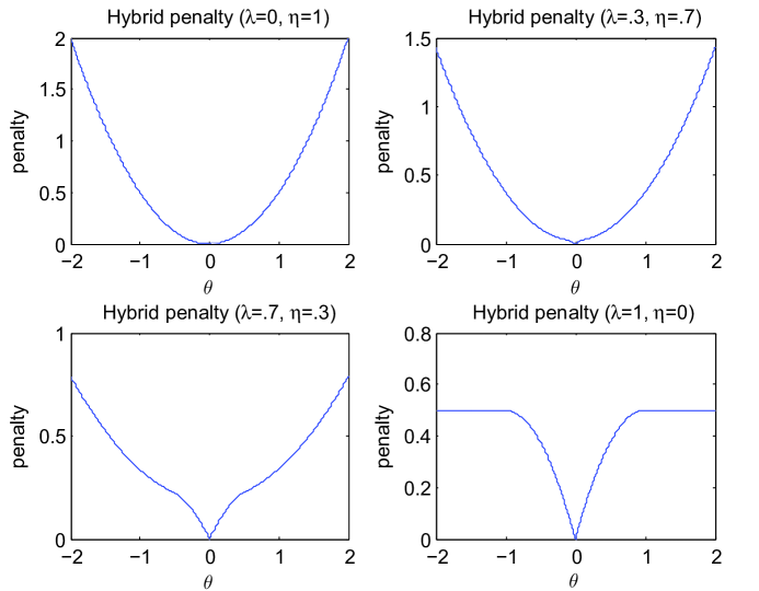
Figure 1: The penalty defined by hybrid-thresholding. As $\lambda$ and $\eta$ vary, it takes the continuous hard-penalty and the ridge penalty as extremes.

Moreover, we have the following nonasymptotic result in parallel to Theorem 4.2. Recall that $k_{0}=\|{\boldsymbol{X}}\|_{2}$, ${\boldsymbol{\Sigma}}^{(s)}={\boldsymbol{\Sigma}}/n={\boldsymbol{X}}^{T}{\boldsymbol{X}}/n$, $\mu=\mu_{\min}({\boldsymbol{\Sigma}}_{nz,nz}^{(s)})$ and $\kappa\triangleq\underset{i\in z}{\max}\|{\boldsymbol{\Sigma}}_{i,nz}^{(s)}\|_{2}/\sqrt{d_{nz}}$. Define $\iota\triangleq\min|({\boldsymbol{\Sigma}}_{nz}+\eta{\boldsymbol{I}})^{-1}{\boldsymbol{\Sigma}}_{nz}{\boldsymbol{\beta}}_{nz}|$, the minimum absolute value in the noiseless partial ridge estimate. Let $p_{e}$ be the probability of Hybrid-TISP estimates having incorrect sparsity patterns, that is, for any $\hat{\boldsymbol{\beta}}\in F$, there exists some $i$ or $j$ such that $\hat{\boldsymbol{\beta}}_{z,i}\neq 0$ or $\hat{\boldsymbol{\beta}}_{nz,j}=0$.

Theorem 5.1.

Assume $\mu>0$, and $\lambda,\eta$ are chosen such that $\kappa\leq\frac{\lambda}{\|{\boldsymbol{\beta}}_{nz}\|_{2}\sqrt{d_{nz}}}\frac{n\mu+\eta}{n\eta}$ and $\iota\geq\frac{\lambda}{k_{0}^{2}+\eta}$. Then

$$p_{e}\leq 2d_{z}\varphi(M^{\prime\prime})/M^{\prime\prime}+2d_{nz}\varphi(L^{\prime\prime})/L^{\prime\prime},$$ (5.3)

where $M^{\prime\prime}=\frac{1}{\sqrt{n}\sigma}\left({\lambda}-\frac{n\eta}{n\mu+\eta}\kappa\|{\boldsymbol{\beta}}_{nz}\|_{2}\sqrt{d_{nz}}\right)$, $L^{\prime\prime}=\frac{n\mu+\eta}{\sqrt{n\mu}\sigma}\left(\iota-\frac{\lambda}{k_{0}^{2}+\eta}\right)$.

Hybrid-TISP successfully offers both selection and shrinkage in estimating ${\boldsymbol{\beta}}$. Before going into the numerical results, we summarize the traits of the design of Hybrid-TISP as follows. (a) Its penalty provides us a trade-off between the $l_{0}$-penalty and the $l_{2}$-penalty (ridge-penalty), and takes the two as extremes, from which we secure selection and shrinkage simultaneously. In particular, the selection is achieved by a penalty more like $l_{0}$ than $l_{1}$, seen from the penalty function, or the iterative thresholding. (b) Hybrid-TISP avoids double shrinkage. Double shrinkage is a serious problem in the design of naive elastic net [39] which simply adopts a linear combination of the $l_{1}$-penalty and the $l_{2}$-penalty. However, the $l_{1}$-penalty also plays a role in shrinking the nonzero coefficients in addition to the $l_{2}$-penalty. By contrast, Hybrid-TISP deals with the zeros and the nonzeros separately, by hard-thresholding and ridge-thresholding, respectively; there is no overlapping between them. (c) We have two parameters, $\lambda$ and $\eta$, responsible for selection and shrinkage respectively. One drawback of the lasso is that it uses the same parameter to control both selection and shrinkage [24]. Therefore, it may result in insufficient zeros even if the SNR is pretty high, as shown clearly in Table 1. Hybrid-TISP has $\lambda$, $\eta$ designed for the two different purposes and can adapt to different sparsity and noise level. (d) The TISP selecting and shrinking interplay with each other during the iteration till in the end we successfully achieve selection/shrinkage balance in the final estimate. This is in contrast to the relaxed lasso [24] which treats selection and shrinkage as separate steps in building a model. (e) Finally, Hybrid-TISP is a very simple procedure to implement. It only involves multiplication and thresholding operations.

In the implementation of Hybrid-TISP, an empirical parameter search is usually needed to determine the values of $\lambda$ and $\eta$, because running a grid search over the $(\lambda,\eta)$-space is a formidable task. We search along a couple of few one-dimensional solution paths including the $\lambda$-paths (with $\eta$ fixed) and the $\eta$-paths (with $\lambda$ fixed) to save computational cost. The optimal tuning parameter from the ridge regression path (corresponding to $\lambda=0$), denoted by $\eta^{(r)}$, is used as a reference for $\eta$. Briefly, our search process generates and searches along some $\lambda$- and $\eta$-paths, compares the results from these searches, and then takes $(\lambda,\eta)$ to be the one minimizing the validation error. The concrete search paths are as follows. (i) $n>p$. Denote the OLS scale estimate by $\hat{\sigma}$. If $n/p<5$, or $n/p<10$ but $\hat{\sigma}>5$, we adopt the alternative search strategy which has been shown to be fast and efficacious [27]: fixing $\eta$ at $0.5\eta^{(r)}$, search along the $\lambda$-path to get an optimal solution (having the smallest validation error) at, say, $\lambda^{(o)}$; then search along the $\eta$-path with $\lambda$ fixed at $\lambda^{(o)}$. If $n/p>10$ and $\hat{\sigma}<5$, we only search over the $\lambda$-path with $\eta=0.05\eta^{(r)}$. In all remaining cases, we generate and search long two $\lambda$-paths with $\eta=0.5\eta^{(r)}$ and $0.05\eta^{(r)}$ respectively. (ii) $p>n$. We use the above alternative search starting with $0.5\eta^{(r)}$, and an additional search for $\lambda$ with $\eta$ fixed at $0.05\eta^{(r)}$. Accordingly, 3 paths in total are generated in the large-$p$ situation. This simple empirical search does not cover the full parameter space but is more efficient than a grid search. The results are reported in Table 1. We also included the elastic net (eNet) in the experiments, which has two regularization parameters as well. Note that eNet generates and searches along 6 solution paths to tune the parameters [39].

Seen from Table 1, Hybrid-TISP has amazing performance in both accuracy and sparsity. We briefly summarize the story as follows. When the noise level is low or medium, the value of $\lambda$ in the lasso is limited by the amount of shrinkage and thus gives insufficient sparsity. Large noise alleviates the problem but there is still much room for the improvement of test-error and sparsity-error because the amount of shrinkage may not equal to the thresholding value in the selection. The weighted lasso like the one-step SCAD has somewhat limited power because the OLS estimate may be inaccurate and misleading for weight construction. Benefiting from the $l_{2}$-penalty, the eNet shows much better accuracy in the case of large noise and/or high correlation between the variables; nevertheless, the sparsity of the estimate may be seriously hurt when the ridge penalty must take control. And it seems possible to improve its test-error further by incorporating this sparsity in estimation. All of these problems can be resolved by Hybrid-TISP, which achieves the right balance between shrinkage and selection. Its test error is consistently lower than the eNet, and more importantly, Hybrid-TISP provides a parsimonious model as Hard-TISP.

5.3 Large sample and large dimension experiments

At the end of this section, we demonstrate the performance of TISP on large-$n$ data as well as on large-$p$ data. We modified the parameters in Example 1 and reran the simulations, where $\Sigma_{ij}=\rho^{|i-j|}$ with $\rho=.5$, ${\boldsymbol{\beta}}$ is appended with zeros given by $[3,1.5,0,0,2,0,0,\cdots,0]^{T}$, $\sigma=2,5$, and $n$, $d$ are not fixed anymore: in the large sample experiment, $d=8$, $n=40,80,200$ (corresponding to $5$ times, $10$ times, and $25$ times as large as $d$); in the large dimension experiment, $n=20$, $d=100,200,500$ (corresponding to $5$ times, $10$ times, and $25$ times as large as $n$). Table 2 shows the simulation results of these different combinations of $n$ and $d$. In both situations, the Hybrid-TISP path is preferable in terms of accuracy and sparsity. Our conclusions are similar to the findings summarized before. Note that one-step SCAD uses the OLS estimate as the initial guess and thus is not included in the large-$p$ simulation. In fact, as an example of the adaptive lasso, it is most powerful in large samples with small noise and low correlation between covariates, where the OLS estimate is accurate. The elastic net is an improvement of the lasso and provides a good algorithm in predictive learning. However, despite having two regularization parameters, it does not improve much the sparsity of the lasso. Hard- and SCAD-IPOD give significantly different solution paths than the above convex penalties. They may dramatically reduce the sparsity error and the test error, say, for large-$p$ sparse signals with moderate noise. Both thresholdings fall into the hard-thresholding family which does not introduce much estimation bias for large coefficients. Interestingly, if our main concern is to reduce the test error in building a statistical model (which is the most frequently used tuning criterion in implementation), they are not always our best choices. Indeed, it is more desirable to offer adaptive shrinkage to nonzero coefficient estimation to benefit from the bias-variance tradeoff. Hybrid-TISP is successful especially for the large-$p$ data because it does joint and adaptive selection and shrinkage.

		Lasso	One-step SCAD	Hard-TISP	SCAD-TISP	eNet	Hybrid-TISP
$n=\textbf{40}$, $d=8$,	Test-err	14.2(2.8)	10.6(2.3)	10.4(2.7)	9.2(1.9)	10.7(2.7)	8.2(2.5)
	Spar-err	29.3	12.5	0.0	4.5	29.7	0.0
$\sigma=2$	Prop-Z	53.0%	91.0 %	100%	100%	52.5%	100.0%
	Prop-NZ	100%	100%	100%	100%	100%	100%
$n=\textbf{40}$, $d=8$,	Test-err	12.6(3.0)	15.2(3.1)	13.9(2.4)	13.3(2.0)	10.0(2.9)	12.3(2.5)
	Spar-err	29.8	25.0	16.9	17.6	31.7	16.9
$\sigma=5$	Prop-Z	54.7%	66.4 %	94.1%	80%	52.0%	93.9%
	Prop-NZ	100%	83.0%	87.7%	83.3%	100.0%	100.0%
$n=\textbf{80}$, $d=8$,	Test-err	9.2(2.6)	5.6(2.0)	5.7(1.8)	5.7(1.9)	8.7(2.8)	5.6(1.8)
	Spar-err	44.3	3.5	0	4.7	42.9	0
$\sigma=2$	Prop-Z	29.2%	94.4%	100%	92.4%	31.3%	100%
	Prop-NZ	100%	100%	100%	100%	100.0%	100%
$n=\textbf{80}$, $d=8$,	Test-err	8.8(2.5)	10.0(2.3)	5.8(1.8)	6.8(1.9)	7.6(2.2)	5.2(1.7)
	Spar-err	44.9	17.8	4.6	17.9	37.5	3.8
$\sigma=5$	Prop-Z	29.2%	80%	94.9%	80%	40.0%	95.1%
	Prop-NZ	100%	100%	100%	100%	100%	100.0%
$n=\textbf{200}$, $d=8$,	Test-err	3.2(1.6)	1.7(1.4)	1.8(1.4)	1.8(1.4)	2.3(1.5)	1.8(1.4)
	Spar-err	43.4	3.2	3.8	2.9	29.8	3.8
$\sigma=2$	Prop-Z	30.5%	94.8%	93.9%	95.3%	52.4%	93.9%
	Prop-NZ	100%	100%	100%	100%	100%	100%
$n=\textbf{200}$, $d=8$,	Test-err	3.2(1.6)	2.5(1.5)	2.2(1.4)	2.7(1.6)	3.0(1.4)	1.9(1.3)
	Spar-err	37.5	17.8	12.5	3.3	29.8	12.5
$\sigma=5$	Prop-Z	40.0%	71.1%	92.4%	98.0%	52.3%	80.0%
	Prop-NZ	100%	100%	100%	100%	100%	100%
$n=20$, $d=\textbf{100}$,	Test-err	83.2(7.9)	——	68.3(10.6)	45.1(8.8)	82.9(7.4)	64.3(10.2)
	Spar-err	7.9	——	1.3	1.0	7.5	1.3
$\sigma=2$	Prop-Z	100%	——	100%	100.0%	100.0%	98.5%
	Prop-NZ	92.0%	——	99.3 %	99.6 %	92.2%	100.0%
$n=20$, $d=\textbf{100}$,	Test-err	50.7(3.7)	——	53.0(7.1)	50.0(6.8)	51.0(4.7)	39.9(6.1)
	Spar-err	7.5	——	3.5	2.3	7.6	2.4
$\sigma=5$	Prop-Z	93.9%	——	99.6%	99.7%	93.2%	98.7%
	Prop-NZ	52.8%	——	49.6%	33.3%	66.7%	66.7%
$n=20$, $d=\textbf{200}$,	Test-err	121.2(15.0)	——	98.0(12.0)	92.3(16.3)	121.6(13.9)	103.9(12.6)
	Spar-err	4.7	——	1.0	0.8	4.2	0.7
$\sigma=2$	Prop-Z	95.4%	——	99.9%	99.9%	95.7%	99.9%
	Prop-NZ	100%	——	84.6%	85.0%	100.0%	66.7%
$n=20$, $d=\textbf{200}$,	Test-err	57.2(5.8)	——	58.6(6.8)	59.8(7.5)	54.1(5.8)	47.7(6.5)
	Spar-err	3.5	——	1.5	1.8	4.6	1.3
$\sigma=5$	Prop-Z	97.5%	——	99.2%	99.3%	95.8%	99.0%
	Prop-NZ	46.0%	——	53.3%	51.6%	66.7%	66.7%
$n=20$, $d=\textbf{500}$,	Test-err	173.5(19.1)	——	117.9(14.6)	118.1(16.3)	181.1(20.1)	118.2(14.5)
	Spar-err	2.5	——	0.4	0.3	2.1	0.4
$\sigma=2$	Prop-Z	97.6%	——	100.0%	100%	97.9%	99.9%
	Prop-NZ	100%	——	66.7%	66.7%	88.4%	66.7%
$n=20$, $d=\textbf{500}$,	Test-err	72.9(7.5)	——	66.6(6.5)	67.5(7.0)	67.3(7.2)	60.1(6.5)
	Spar-err	1.2	——	0.7	0.7	1.4	1.1
$\sigma=5$	Prop-Z	99.2%	——	99.5%	99.6%	99.0%	99.3%
	Prop-NZ	33.3%	——	50.6%	50.0%	33.3%	51.3%

Table 2: Performance comparisons on the simulation data with large sample size or dimensionality, in terms of test error, sparsity error, proper sparsity, and proper nonsparsity over 50 simulations. Six methods are listed here: lasso (Soft-TISP), one-step SCAD, Hard-TISP, SCAD-TISP, elastic net (eNet), and Hybrid-TISP; the last two both have two regularization parameters.

6 Real Data

Hybrid-TISP was applied to a real prostate dataset which was used by Tibshirani [30]. The prostate data have $97$ observations and $9$ clinical measures. In this example, unlike [30], we take the log(cancer volume) (lcavol) as the response variable and consider a full quadratic model; the $43$ predictors are $8$ main effects, $7$ squares, and $28$ interactions of eight original variables — lweight, age, lbph, svi, lcp, gleason, pgg45, and lpsa, where svi is binary. The lasso does not give stable and accurate results for this example due to the existence of many highly correlated predictors.

The regularization parameters of Hybrid-TISP were tuned by leave-one-out cross-validation. To identify the relevant variables in a trustworthy way, nonparametric bootstrap resampling was used with $B=100$. For every bootstrap dataset, after standardizing the predictors, we apply Hybrid-TISP with fixed regularization parameters tuned for the original dataset. Figure 3 shows the percentages of the bootstrap coefficient estimates being nonzero over the $100$ replications for all the $43$ predictors. The histograms are plotted in Figure 2. It is easy to see that $8$ variables are much more significant than the others. In fact, these are exactly the variables selected by Hybrid-TISP on the original data. A more careful examination shows that they appear (jointly) $36$ times in the selected models, the top visited octuple in bootstrapping. These variables fall into two groups with similar patterns: (I) $\{x_{5},x_{19},x_{25},x_{38}\}$, i.e., {lcp, lweight*lcp, age*lcp, gleason*lcp}; (II) $\{x_{8},x_{22},x_{28},x_{42}\}$, i.e., {lpsa, lweght*lpsa, age*lpsa, gleason*lpsa}. The within-group correlations are very high, $>.98$ for Group (I), and $>.93$ for Group (II). Furthermore, an interesting feature is that for any of the eight variables selected by Hybrid-TISP, the other three in the same group are most correlated with it among $42$ predictors.

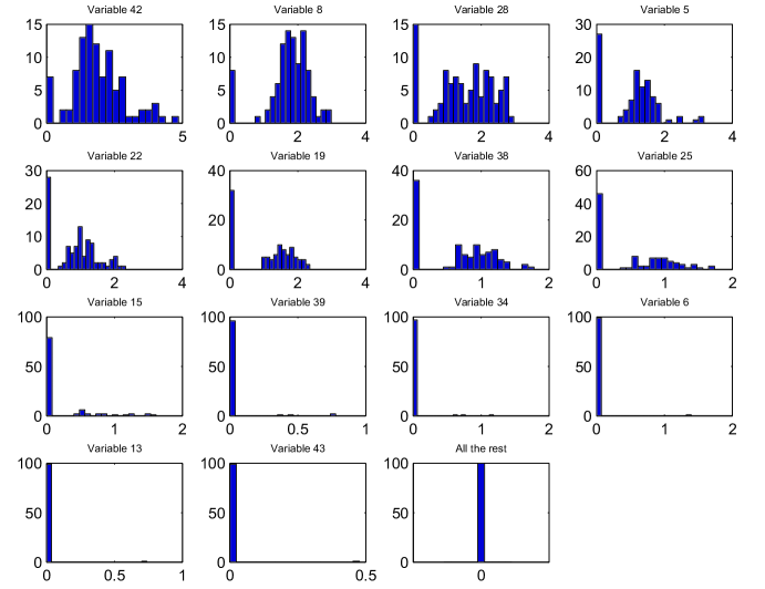
Figure 2: Histograms of the $100$ Hybrid-TISP coefficient estimates for all of the $43$ predictors in the prostate example.

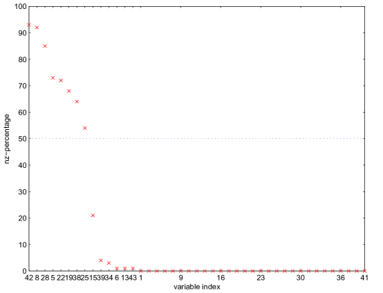
Figure 3: Proportions of the Hybrid-TISP coefficients being nonzero over the $100$ bootstrap replications in the prostate example. Eight variables have nonzero coefficient estimates more frequently than zero estimates.

7 Discussion

We have proposed the thresholding-based iterative selection procedures for solving nonconvex penalized regressions. In fact, people have long before noticed the weakness of the convex $l_{1}$-constraint (or the soft-thresholding) in wavelets and have designed many different forms of nonconvex penalties to increase model sparsity and accuracy. But for a nonorthogonal regression matrix, there is great difficulty in both investigating the performance in theory and solving the problem in computation. TISP provides a simple and efficient way to tackle this.

Somewhat different than other studies, we started from thresholding rules rather than penalty functions. Indeed, there is a universal connection between them. But a drawback of the latter is its non-unique form: different penalties may result in the same estimator and the same thresholding. The main contribution of this paper is the study of a class of $\Theta$-estimators satisfying (3.11), which can be naturally computed by TISP, and are associated with penalized regressions. With a carefully designed thresholding rule, we obtained a good estimator for model selection and shrinkage. Starting from $\Theta$ greatly facilitated the computation and the analysis. In fact, some penalty designs may even have a better explanation from $\Theta$, or equivalently, the $\psi$-function — for example, the SCAD-penalty (recall that it is defined by its derivative) seems to originate from Hampel’s three-part redescending $\psi$. Conversely, we can use TISP to compute $M$-estimators in robust statistics as described in Section 3.3.

Using a thresholding rule in the hard-thresholding family, TISP gives good selection results. Our novel Hybrid-TISP, accomplishing a fusion between $l_{0}$-penalty and $l_{2}$-penalty based on the hard-thresholding and the ridge thresholding, shows superior performance and beats the commonly used methods in both test-error and sparsity. The hybrid penalty function (5.2) may look a bit odd, but is quite natural and simple from the point of view of thresholding; see (5.1). It is worth mentioning that in contrast to [19, 3, 2], where more than one tuning parameter is considered a drawback and unnecessity, we believe a good procedure should have two explicit regularization parameters to control and balance selection and shrinkage.

We assume the penalty function $P$ is dependent on ${\boldsymbol{\beta}}$ and $\lambda$ only. Therefore the iterative weighting, substituting the nonnegative garrote [19] for $\Theta$ in TISP, is not covered by the studies in this paper. In fact, with ${\boldsymbol{\beta}}$ involved in $P$, it might be difficult to optimize in the second step of the mechanism introduced in Section 2.

The solution path associated with a nonconvex penalty is generally not continuous in $\lambda$. For example, even for the transformed $l_{1}$-penalty in Example 3 which is differentiable to any order on $(0,+\infty)$, the solution path still has no $\lambda$-continuity practically. Hence a pathwise algorithm is not appropriate here. Empirically, using a zero estimate as the start in nonconvex TISPs works pretty well. We conjecture that it leads to an estimate with some least norm property. Take Hard-IPOD as an example: this roughly means that we were looking for the local minimum of the $l_{0}$-penalized regression that is closest to zero in building a parsimonious model.

The generalization of TISP to GLM seems straightforward; we will investigate this topic in the next paper. TISP fits perfectly into the Accelerated Annealing [27] and thus can be used in the generic sparse regression with customizable sparsity patterns, such as the supervised clustering problem. Other future studies include developing some acceleration techniques for TISP (like the relaxation and asynchronous updating [27]) and deriving some risk oracles in theory.

Appendix A Proofs

A.1 Proofs of Theorem 3.1, Proposition 3.2, and Proposition 3.3

Let’s consider the orthogonal case first. Define $Q({\boldsymbol{\gamma}})=\|{\boldsymbol{\gamma}}-{\boldsymbol{\alpha}}\|_{2}^{2}/2+P({\boldsymbol{\gamma}};\lambda)$, where ${\boldsymbol{\alpha}}$ is a known vector. Let ${\boldsymbol{\gamma}}_{o}=\arg\min Q({\boldsymbol{\gamma}})$. By the construction of $P$ and Proposition 3.1, ${\boldsymbol{\gamma}}_{o}$ satisfies ${\boldsymbol{\gamma}}_{o}-{\boldsymbol{\alpha}}+s({\boldsymbol{\gamma}}_{o};\lambda)=\boldsymbol{0}$.

$$Q({\boldsymbol{\gamma}}_{o}+\boldsymbol{h})-Q({\boldsymbol{\gamma}}_{o}) = \frac{1}{2}\|{\boldsymbol{\gamma}}_{o}+\boldsymbol{h}-{\boldsymbol{\alpha}}\|_{2}^{2}-\frac{1}{2}\|{\boldsymbol{\gamma}}_{o}-{\boldsymbol{\alpha}}\|_{2}^{2}+P({\boldsymbol{\gamma}}_{o}+\boldsymbol{h};\lambda)-P({\boldsymbol{\gamma}}_{o};\lambda)$$

$$= \frac{1}{2}\|\boldsymbol{h}\|_{2}^{2}+<\boldsymbol{h},{\boldsymbol{\gamma}}_{o}-{\boldsymbol{\alpha}}>+P({\boldsymbol{\gamma}}_{o}+\boldsymbol{h};\lambda)-P({\boldsymbol{\gamma}}_{o};\lambda)$$

$$= \frac{1}{2}\|\boldsymbol{h}\|_{2}^{2}+\left(P({\boldsymbol{\gamma}}_{o}+\boldsymbol{h};\lambda)-P({\boldsymbol{\gamma}}_{o};\lambda)-<\boldsymbol{h},\boldsymbol{s}>\right)$$

$$\geq \frac{1}{2}\|\boldsymbol{h}\|_{2}^{2}-\frac{1}{2}\boldsymbol{h}^{T}{\boldsymbol{H}}\boldsymbol{h}=\frac{1}{2}\boldsymbol{h}^{T}({\boldsymbol{I}}-{\boldsymbol{H}})\boldsymbol{h}.$$

This inequality is due to the BCC (3.7). On the other hand, we know

$$Q({\boldsymbol{\gamma}}_{o}+\boldsymbol{h})-Q({\boldsymbol{\gamma}}_{o})\geq 0.$$

In summary, we get

$$Q({\boldsymbol{\gamma}}_{o}+\boldsymbol{h})-Q({\boldsymbol{\gamma}}_{o})\geq\frac{1}{2}\boldsymbol{h}^{T}{\boldsymbol{A}}\boldsymbol{h},$$ (A.1)

for both ${\boldsymbol{A}}={\boldsymbol{I}}-{\boldsymbol{H}}$ and ${\boldsymbol{A}}=\boldsymbol{0}$; formally, we write ${\boldsymbol{A}}=({\boldsymbol{I}}-{\boldsymbol{H}})\vee\boldsymbol{0}$. Note that (A.1) is a global result for any $\boldsymbol{h}$.

Now look at the TISP. Recall the $g$ in (2.2) is

$$g({\boldsymbol{\beta}},{\boldsymbol{\gamma}})=\frac{1}{2}\|{\boldsymbol{X}}{\boldsymbol{\gamma}}-{\boldsymbol{y}}\|_{2}^{2}+P({\boldsymbol{\gamma}};\lambda)+\frac{1}{2}({\boldsymbol{\gamma}}-{\boldsymbol{\beta}})^{T}({\boldsymbol{I}}-{\boldsymbol{\Sigma}})({\boldsymbol{\gamma}}-{\boldsymbol{\beta}}).$$

Then given ${\boldsymbol{\beta}}$, we can write $g$ as

$$g({\boldsymbol{\beta}},{\boldsymbol{\gamma}})=\frac{1}{2}\|{\boldsymbol{\gamma}}-(({\boldsymbol{I}}-{\boldsymbol{\Sigma}}){\boldsymbol{\beta}}+{\boldsymbol{X}}^{T}{\boldsymbol{y}})\|_{2}^{2}+C({\boldsymbol{X}},{\boldsymbol{y}},{\boldsymbol{\beta}}),$$

and apply (A.1) with ${\boldsymbol{\alpha}}=({\boldsymbol{I}}-{\boldsymbol{\Sigma}}){\boldsymbol{\beta}}+{\boldsymbol{X}}^{T}{\boldsymbol{y}}$,

$$g({\boldsymbol{\beta}},{\boldsymbol{\gamma}}_{o}({\boldsymbol{\beta}})+\boldsymbol{h})-g({\boldsymbol{\beta}},{\boldsymbol{\gamma}}_{o}({\boldsymbol{\beta}}))\geq\frac{1}{2}{\boldsymbol{h}}^{T}(({\boldsymbol{I}}-{\boldsymbol{H}})\vee\boldsymbol{0}){\boldsymbol{h}},\quad\forall{\boldsymbol{h}}.$$ (A.2)

Correspondingly, for the TISP iterates ${\boldsymbol{\beta}}^{(j)}$, we have

$$f({\boldsymbol{\beta}}^{(j+1)})+\frac{1}{2}({\boldsymbol{\beta}}^{(j+1)}-{\boldsymbol{\beta}}^{(j)})^{T}({\boldsymbol{I}}-{\boldsymbol{\Sigma}})({\boldsymbol{\beta}}^{(j+1)}-{\boldsymbol{\beta}}^{(j)})=g({\boldsymbol{\beta}}^{(j)},{\boldsymbol{\beta}}^{(j+1)})$$

$$\leq g({\boldsymbol{\beta}}^{(j)},{\boldsymbol{\beta}}^{(j)})-\frac{1}{2}({\boldsymbol{\beta}}^{(j+1)}-{\boldsymbol{\beta}}^{(j)})^{T}(({\boldsymbol{I}}-{\boldsymbol{H}})\vee\boldsymbol{0})({\boldsymbol{\beta}}^{(j+1)}-{\boldsymbol{\beta}}^{(j)})$$

$$= f({\boldsymbol{\beta}}^{(j)})-\frac{1}{2}({\boldsymbol{\beta}}^{(j+1)}-{\boldsymbol{\beta}}^{(j)})^{T}(({\boldsymbol{I}}-{\boldsymbol{H}})\vee\boldsymbol{0})({\boldsymbol{\beta}}^{(j+1)}-{\boldsymbol{\beta}}^{(j)}).$$

That is,

$$f({\boldsymbol{\beta}}^{(j)})-f({\boldsymbol{\beta}}^{(j+1)})\geq\frac{1}{2}({\boldsymbol{\beta}}^{(j+1)}-{\boldsymbol{\beta}}^{(j)})^{T}(({\boldsymbol{I}}-{\boldsymbol{H}})\vee\boldsymbol{0}+{\boldsymbol{I}}-{\boldsymbol{\Sigma}})({\boldsymbol{\beta}}^{(j+1)}-{\boldsymbol{\beta}}^{(j)}).$$ (A.3)

Now (3.8) and (3.9) can be obtained after simple calculations.

As for Proposition 3.2, let ${\boldsymbol{\beta}}^{(j_{k})}\rightarrow{\boldsymbol{\beta}}^{*}$ as $k\rightarrow\infty$. Under the condition $\mu_{\max}({\boldsymbol{\Sigma}})<1\vee(2-\mu_{\max}({\boldsymbol{H}}))$, Theorem 3.1 states that

$$\|{\boldsymbol{\beta}}^{(j_{k}+1)}-{\boldsymbol{\beta}}^{(j_{k})}\|_{2}^{2}\leq(f({\boldsymbol{\beta}}^{(j_{k})})-f({\boldsymbol{\beta}}^{(j_{k}+1)}))/C\leq(f({\boldsymbol{\beta}}^{(j_{k})})-f({\boldsymbol{\beta}}^{(j_{k+1})}))/C\rightarrow 0.$$

That is, $\Theta(({\boldsymbol{I}}-{\boldsymbol{\Sigma}}){\boldsymbol{\beta}}^{(j_{k})}+{\boldsymbol{X}}^{T}{\boldsymbol{y}};\lambda)-{\boldsymbol{\beta}}^{(j_{k})}\rightarrow 0$. Therefore, ${\boldsymbol{\beta}}^{*}$ is a fixed point of TISP.

Finally, we prove Proposition 3.3. Noticing that ${\boldsymbol{\gamma}}_{o}({\boldsymbol{\beta}}^{*})={\boldsymbol{\beta}}^{*}$, we get the following inequality from (A.2)

$$g({\boldsymbol{\beta}}^{*},{\boldsymbol{\beta}}^{*}+{\boldsymbol{h}})-g({\boldsymbol{\beta}}^{*},{\boldsymbol{\beta}}^{*})\geq\frac{1}{2}{\boldsymbol{h}}^{T}(({\boldsymbol{I}}-{\boldsymbol{H}})\vee\boldsymbol{0}){\boldsymbol{h}},\quad\forall{\boldsymbol{h}}.$$

Since $g({\boldsymbol{\beta}}^{*},{\boldsymbol{\beta}}^{*})=f({\boldsymbol{\beta}}^{*})$,

$$f({\boldsymbol{\beta}}^{*}+{\boldsymbol{h}})+\frac{1}{2}{\boldsymbol{h}}^{T}({\boldsymbol{I}}-{\boldsymbol{\Sigma}}){\boldsymbol{h}}\geq f({\boldsymbol{\beta}}^{*})+\frac{1}{2}{\boldsymbol{h}}^{T}(({\boldsymbol{I}}-{\boldsymbol{H}})\vee\boldsymbol{0}){\boldsymbol{h}},\quad\forall{\boldsymbol{h}}$$

$$\Rightarrow f({\boldsymbol{\beta}}^{*}+{\boldsymbol{h}})-f({\boldsymbol{\beta}}^{*})\geq\frac{1}{2}{\boldsymbol{h}}^{T}(({\boldsymbol{I}}-{\boldsymbol{H}})\vee\boldsymbol{0}+{\boldsymbol{\Sigma}}-{\boldsymbol{I}}){\boldsymbol{h}},\quad\forall{\boldsymbol{h}}.$$

Therefore, if $\mu({\boldsymbol{\Sigma}})\geq\mu_{\max}({\boldsymbol{H}})$, ${\boldsymbol{\beta}}^{*}$ is a global minimizer of $f$.

A.2 Proofs of Theorem 4.1 and Theorem 4.2

These theorems have all been essentially proved in [27]. We provide a self-contained proof as follows. All inequalities and the absolute value ‘$||$’ are understood in the componentwise sense. Assume, for the moment, ${\boldsymbol{X}}$ has been column-normalized such that the diagonal entries of ${\boldsymbol{\Sigma}}={\boldsymbol{X}}^{T}{\boldsymbol{X}}$ are all 1. Let ${\boldsymbol{\Sigma}}_{I}={\boldsymbol{X}}_{I}^{T}{\boldsymbol{X}}_{I}$, ${\boldsymbol{\Sigma}}_{I,I^{\prime}}={\boldsymbol{X}}_{I}^{T}{\boldsymbol{X}}_{I^{\prime}}$ for any index sets $I,I^{\prime}$.

Lemma A.1.

Assume ${\boldsymbol{\Sigma}}_{nz}$ is nonsingular. The TISP estimate $\hat{\boldsymbol{\beta}}$ satisfies the following equations

$${\boldsymbol{S}}_{z}\hat{\boldsymbol{\beta}}_{z}=({\boldsymbol{X}}_{z}^{T}-{\boldsymbol{\Sigma}}_{z,nz}{\boldsymbol{\Sigma}}_{nz}^{-1}{\boldsymbol{X}}_{nz}^{T}){\boldsymbol{\epsilon}}+\tau{\boldsymbol{\Sigma}}_{z,nz}{\boldsymbol{\Sigma}}_{nz}^{-1}\widetilde{{\mbox{sgn}}}(\hat{\boldsymbol{\beta}}_{nz};{\lambda}/{k_{0}^{2}})-\tau\widetilde{{\mbox{sgn}}}(\hat{\boldsymbol{\beta}}_{z};{\lambda}/{k_{0}^{2}})$$ (A.4)

$$\hat{\boldsymbol{\beta}}_{nz}={\boldsymbol{\beta}}_{nz}+{\boldsymbol{\Sigma}}_{nz}^{-1}({\boldsymbol{X}}_{nz}^{T}{\boldsymbol{\epsilon}}-\tau\widetilde{{\mbox{sgn}}}(\hat{\boldsymbol{\beta}}_{nz};{\lambda}/{k_{0}^{2}}))-{\boldsymbol{\Sigma}}_{nz}^{-1}{\boldsymbol{\Sigma}}_{z,nz}^{T}\hat{\boldsymbol{\beta}}_{z}$$ (A.5)

where ${\boldsymbol{S}}_{z}={\boldsymbol{\Sigma}}_{z}-{\boldsymbol{\Sigma}}_{z,nz}{\boldsymbol{\Sigma}}_{nz}^{-1}{\boldsymbol{\Sigma}}_{nz,z}$.

This can be obtained directly from (4.2).

Lemma A.2.

Let $\boldsymbol{z}\sim N(\boldsymbol{0},\boldsymbol{D}_{d\times d})$, $\boldsymbol{z}^{\prime}\sim N(\boldsymbol{0},\boldsymbol{\Lambda}_{d\times d})$, where $\boldsymbol{D}$ is a diagonal matrix. Assume the diagonal entries of $\boldsymbol{\Lambda}$, denoted by $\mbox{diag}(\boldsymbol{\Lambda})$, are the same as those of $\boldsymbol{D}$, i.e., $\mbox{diag}(\boldsymbol{\Lambda})=\mbox{diag}(\boldsymbol{D})$. Then

$$P(\max|\boldsymbol{z}^{\prime}|\geq c)\leq P(\max|\boldsymbol{z}|\geq c),$$ (A.6)

for any $c$.

This is clear from Šidák’s classical result [31] in 1967.

To prove Theorem 4.1, let ${{\boldsymbol{X}}_{z}^{\prime}}^{T}={\boldsymbol{X}}_{z}^{T}-{\boldsymbol{\Sigma}}_{z,nz}{\boldsymbol{\Sigma}}_{nz}^{-1}{\boldsymbol{X}}_{nz}^{T}$ and define

$$A \triangleq \left\{\left|{\boldsymbol{X}}_{z}^{\prime}{\boldsymbol{\epsilon}}+\tau{\boldsymbol{\Sigma}}_{z,nz}{\boldsymbol{\Sigma}}_{nz}^{-1}\widetilde{{\mbox{sgn}}}(\hat{\boldsymbol{\beta}}_{nz})\right|\leq\tau\right\}$$

$$V \triangleq \left\{\left|{\boldsymbol{\Sigma}}_{nz}^{-1}{\boldsymbol{X}}_{nz}^{T}{\boldsymbol{\epsilon}}\right|+\tau\left|{\boldsymbol{\Sigma}}_{nz}^{-1}\boldsymbol{s}\right|<\left|{\boldsymbol{\beta}}_{nz}\right|{\mbox{ for any }}\boldsymbol{s}{\mbox{ satisfying }}|\boldsymbol{s}|\leq 1\right\}.$$

Clearly $1-p_{s}\leq P(A^{c}\cup V^{c})\leq P(A^{c})+P(V^{c})$.

Let ${\boldsymbol{\Sigma}}_{z,nz}=[\boldsymbol{v}_{1},\cdots\boldsymbol{v}_{d_{z}}]^{T}$, then $\|\boldsymbol{v}_{i}\|_{2}\leq\kappa\sqrt{d_{nz}}$. So $|\boldsymbol{v}_{i}^{T}{\boldsymbol{\Sigma}}_{nz}^{-1}\widetilde{{\mbox{sgn}}}(\hat{\boldsymbol{\beta}}_{nz})|\leq\|\boldsymbol{v}_{i}\|_{2}\cdot\|{\boldsymbol{\Sigma}}_{nz}^{-1}\|_{2}\cdot\|\widetilde{{\mbox{sgn}}}(\hat{\boldsymbol{\beta}}_{nz})\|_{2}\leq\kappa d_{nz}/\mu$ and $\left|{\boldsymbol{\Sigma}}_{z,nz}{\boldsymbol{\Sigma}}_{nz}^{-1}\widetilde{{\mbox{sgn}}}(\hat{\boldsymbol{\beta}}_{nz})\right|\leq\kappa d_{nz}/\mu$. It follows that $P(A^{c})\leq P\left(\left\{\max\left|{{\boldsymbol{X}}_{z}^{\prime}}^{T}{\boldsymbol{\epsilon}}\right|\geq(1-\kappa d_{nz}/\mu)\tau\right\}\right).$

Define ${\boldsymbol{\epsilon}}_{1}^{\prime}={{\boldsymbol{X}}_{z}^{\prime}}^{T}{\boldsymbol{\epsilon}}\in\Re^{d_{z}}.$ Note that ${{\boldsymbol{X}}_{z}^{\prime}}^{T}{{\boldsymbol{X}}_{z}^{\prime}}={\boldsymbol{S}}_{z}$. Thus ${\boldsymbol{\epsilon}}_{1}^{\prime}\sim N(\boldsymbol{0},\sigma^{2}{\boldsymbol{S}}_{z})$. Since $\mbox{diag}({\boldsymbol{\Sigma}}_{z})=\boldsymbol{1}$ and $\mbox{diag}({\boldsymbol{\Sigma}}_{z,nz}{\boldsymbol{\Sigma}}_{nz}^{-1}{\boldsymbol{\Sigma}}_{z,nz}^{T})=\left[\boldsymbol{v}_{i}^{T}{\boldsymbol{\Sigma}}_{nz}^{-1}\boldsymbol{v}_{i}\right]\geq\boldsymbol{0}$, $\mbox{diag}({\boldsymbol{S}}_{z})\leq\boldsymbol{1}$. Lemma A.2 states that

$$P(A^{c}) \leq P\left(\max|{\boldsymbol{\epsilon}}_{1}^{\prime\prime}|\cdot\sigma\geq\tau(1-\frac{\kappa d_{nz}}{\mu})\right)$$

$$\leq d_{z}P\left(|\epsilon_{1,i}^{\prime\prime}|\geq\tau(1-\frac{\kappa d_{nz}}{\mu})\frac{1}{\sigma}\right)\equiv 2d_{z}\Phi([M,+\infty)),$$

where ${\boldsymbol{\epsilon}}_{1}^{\prime\prime}\sim N(\boldsymbol{0},\boldsymbol{I}_{d_{z}\times d_{z}})$. Using the standard bound of the normal tail probability, we get $P(A^{c})\leq 2d_{z}\varphi(M)/M,$ where $M=\left(1-\frac{\kappa d_{nz}}{\mu}\right)\frac{\tau}{\sigma}$.

To bound $P(V^{c})$, suppose the spectral decomposition of ${\boldsymbol{\Sigma}}_{nz}$ is given by ${\boldsymbol{\Sigma}}_{nz}=\boldsymbol{U}\boldsymbol{D}\boldsymbol{U}^{T}$ with $\boldsymbol{U}=[\boldsymbol{u}_{1},\cdots,\boldsymbol{u}_{d_{nz}}]^{T}$, then we can represent ${\boldsymbol{\Sigma}}_{nz}^{-1}$ as $\left[\boldsymbol{u}_{i}^{T}\boldsymbol{D}^{-1}\boldsymbol{u}_{j}\right]_{d_{nz}\times d_{nz}}$, and ${\boldsymbol{\Sigma}}_{nz}^{-1}\boldsymbol{s}$ as $\left[\sum_{j=1}^{d_{nz}}s_{j}\boldsymbol{u}_{i}^{T}\boldsymbol{D}^{-1}\boldsymbol{u}_{j}\right]_{d_{nz}\times 1}$. It follows that $\mbox{diag}({\boldsymbol{\Sigma}}_{nz}^{-1})\leq\frac{1}{\mu}$ and $|{\boldsymbol{\Sigma}}_{nz}^{-1}\boldsymbol{s}|\leq\frac{d_{nz}}{\mu}$. Therefore, $P(V^{c})\leq P\left(\left|{\boldsymbol{\Sigma}}_{nz}^{-1}{\boldsymbol{X}}_{nz}^{T}{\boldsymbol{\epsilon}}\right|\leq L_{0}\right),$ where $L_{0}=\min|{\boldsymbol{\beta}}_{nz}|-\tau d_{nz}/\mu$.

Because ${\boldsymbol{\Sigma}}_{nz}^{-1}{\boldsymbol{X}}_{nz}^{T}{\boldsymbol{\epsilon}}\sim N(\boldsymbol{0},\sigma^{2}{\boldsymbol{\Sigma}}_{nz}^{-1})$, and we have shown $\mbox{diag}({\boldsymbol{\Sigma}}_{nz}^{-1})\leq\frac{1}{\mu}$, applying Lemma A.2 yields

$$P(V^{c})=P(\max\left|{\boldsymbol{\Sigma}}_{nz}^{-1}{\boldsymbol{X}}_{nz}^{T}{\boldsymbol{\epsilon}}\right|\geq L_{0})\leq P(\max|{\boldsymbol{\epsilon}}_{2}^{\prime\prime}|\geq L_{0}\frac{\sqrt{\mu}}{\sigma})\leq 2d_{nz}\Phi([L,\infty)),$$

where ${\boldsymbol{\epsilon}}_{2}^{\prime\prime}\sim N(\boldsymbol{0},\boldsymbol{I}_{d_{nz}\times d_{nz}})$. Hence,

$$1-p_{e}\leq P(A^{c}\cup V^{c})\leq P(A^{c})+P(V^{c})\leq 2d_{z}\frac{1}{M}\varphi(M)+2d_{nz}\frac{1}{L}\varphi(L),$$ (A.7)

where $L=\frac{\sqrt{\mu}}{\sigma}\left(\min|{\boldsymbol{\beta}}_{nz}|-\frac{\tau d_{nz}}{{\mu}}\right)$.

In fact, we can get something slightly stronger than (A.7). Observing that ${{\boldsymbol{X}}_{z}^{\prime}}^{T}{\boldsymbol{\epsilon}}$ is independent of ${\boldsymbol{X}}_{nz}^{T}{\boldsymbol{\epsilon}}$, we have

$$p_{s}\geq P(A\cap V)=P(A)\cdot P(V)\geq\left[1-2\Phi(-M)\right]^{d_{z}}\left[1-2\Phi(-L)\right]^{d_{nz}}.$$ (A.8)

(A.8) implies (A.7).

We assumed ${\boldsymbol{x}}_{i}^{T}{\boldsymbol{x}}_{i}=1$ $i=1,\cdots,d$ in the above derivation. If the $l_{2}$-norm of each column of ${\boldsymbol{X}}$ is no greater than $\sigma_{\max}$, we only need to replace ${\boldsymbol{\beta}}$, $\hat{\boldsymbol{\beta}}$, $\tau$, by ${\boldsymbol{\beta}}\cdot\sigma_{\max}$, $\hat{\boldsymbol{\beta}}\cdot\sigma_{\max}$, $\tau/\sigma_{\max}$, respectively. The proof of Theorem 4.1 is now complete if $\sigma_{\max}=\sqrt{n}$.

For Theorem 4.2, noticing that (a) ${\widetilde{\mbox{sgn}}}(u)=0,\forall|u|>c\tau$ by definition and (b) $p_{s}\geq P\left(\hat{\boldsymbol{\beta}}_{z}^{(s)}=0,\mbox{ and }|\hat{\boldsymbol{\beta}}_{nz}^{(s)}|>c\tau^{(s)}\right)$ with ${\boldsymbol{\beta}}^{(s)}={\boldsymbol{\beta}}\sqrt{n}$, $\tau^{(s)}=\tau/\sqrt{n}$, we can prove it following the same lines.

A.3 Proof of Theorem 4.3

Use the same symbols and notations as defined in Appendix A.2. Let $r_{z}=\|\hat{\boldsymbol{\beta}}_{z}\|_{2}^{2}$, $r_{nz}=\|\hat{\boldsymbol{\beta}}_{nz}-{\boldsymbol{\beta}}_{nz}\|_{2}^{2}$. From (A.5), we have

$$R_{nz}\leq 3\left(E\|{\boldsymbol{\Sigma}}_{nz}^{-1}{\boldsymbol{X}}_{nz}^{T}{\boldsymbol{\epsilon}}\|_{2}^{2}+\tau^{2}E\|{\boldsymbol{\Sigma}}_{nz}^{-1}\widetilde{{\mbox{sgn}}}(\hat{\boldsymbol{\beta}}_{nz})\|_{2}^{2}+\kappa^{2}\frac{d_{z}d_{nz}}{\mu^{2}}\cdot R_{z}\right),$$

due to Cauchy-Schwarz inequality and the fact that $\|{\boldsymbol{\Sigma}}_{z,nz}\|_{2}=\underset{\|\boldsymbol{\alpha}\|_{2}=1}{\max}\|{\boldsymbol{\Sigma}}_{z,nz}\boldsymbol{\alpha}\|_{2}\leq\kappa\sqrt{d_{z}d_{nz}}$. Thus $R_{nz}\leq 3\left(\sigma^{2}tr({\boldsymbol{\Sigma}}_{nz}^{-1})+\tau^{2}\frac{d_{nz}}{\mu^{2}}+\kappa^{2}\frac{d_{z}d_{nz}}{\mu^{2}}\cdot R_{z}\right)$ and (4.8) holds.

To get (4.9), we need the following result about $\mu_{max}({\boldsymbol{S}}_{z}^{-1})$, the largest eigenvalue of ${\boldsymbol{S}}_{z}^{-1}$: $\mu_{max}({\boldsymbol{S}}_{z}^{-1})\leq\frac{1}{\nu}\left(1-\kappa^{2}\cdot\frac{d_{z}d_{nz}}{\mu\nu}\right)^{-1}.$ This is true by noting that ${\boldsymbol{S}}_{z}={{\boldsymbol{X}}_{z}^{\prime}}^{T}{{\boldsymbol{X}}_{z}^{\prime}}$ is semi-positive definite and $\mu_{min}({\boldsymbol{S}}_{z})\geq\nu-\kappa^{2}d_{z}d_{nz}/\mu$.

By (A.4) and the results in Appendix A.2, we have

$$r_{z} \leq 3\mu_{max}^{2}({\boldsymbol{S}}_{z}^{-1})\left[\|{{\boldsymbol{X}}_{z}^{\prime}}^{T}{\boldsymbol{\epsilon}}\|_{2}^{2}+\tau^{2}\|{\boldsymbol{\Sigma}}_{z,nz}{\boldsymbol{\Sigma}}_{nz}^{-1}\widetilde{{\mbox{sgn}}}(\hat{\boldsymbol{\beta}}_{nz})\|_{2}^{2}+\tau^{2}\|\widetilde{{\mbox{sgn}}}(\hat{\boldsymbol{\beta}}_{z})\|_{2}^{2}\right]\cdot 1_{A^{c}}$$

$$\leq 3\mu_{max}^{2}({\boldsymbol{S}}_{z}^{-1})\left[\|{{\boldsymbol{X}}_{z}^{\prime}}^{T}{\boldsymbol{\epsilon}}\|_{2}^{2}\cdot 1_{A^{c}}+\left(\tau^{2}d_{z}\cdot\kappa^{2}\frac{d_{nz}^{2}}{\mu^{2}}+\tau^{2}d_{z}\right)\cdot 1_{A^{c}}\right].$$

Therefore,

$$R_{z} \leq 3\mu_{max}^{2}({\boldsymbol{S}}_{z}^{-1})\left[E(\|{{\boldsymbol{X}}_{z}^{\prime}}^{T}{\boldsymbol{\epsilon}}\|_{2}^{2}\cdot 1_{A^{c}})+\left(1+\kappa^{2}\frac{d_{nz}^{2}}{\mu^{2}}\right)\tau^{2}d_{z}\cdot 2d_{z}\frac{1}{M}\varphi(M)\right]$$

$$\leq 3\mu_{max}^{2}({\boldsymbol{S}}_{z}^{-1})\cdot d_{z}E\left[(\max|{\boldsymbol{\epsilon}}_{1}^{\prime}|)^{2};\max|{\boldsymbol{\epsilon}}_{1}^{\prime}|\geq\tau(1-\kappa\frac{d_{nz}}{\mu})\right]+$$

$$3\mu_{max}^{2}({\boldsymbol{S}}_{z}^{-1})\cdot\frac{1+\kappa^{2}d_{nz}^{2}/\mu^{2}}{(1-\kappa d_{nz}/\mu)^{2}}\cdot 2\sigma^{2}d_{z}^{2}M\varphi(M).$$

Since for a random variable $z$ with probability density $p(\cdot)$ and $a>0$,

$$E(z^{2};z\geq a)=\int_{a}^{\infty}t^{2}p(t)dt=\int_{a}^{\infty}2sP(z\geq s)ds+a^{2}P(z\geq a),$$

it follows from Lemma A.2 that

$$E\left[(\max|{\boldsymbol{\epsilon}}_{1}^{\prime}|)^{2};\max|{\boldsymbol{\epsilon}}_{1}^{\prime}|\geq\tau(1-\kappa\frac{d_{nz}}{\mu})\right]\leq E\left[\max|{\boldsymbol{\epsilon}}_{1}^{\prime\prime}|^{2}\cdot\sigma^{2};\max|{\boldsymbol{\epsilon}}_{1}^{\prime\prime}|\geq M\right].$$

(Recall that ${\boldsymbol{\epsilon}}_{1}^{\prime\prime}\sim N(\boldsymbol{0},\boldsymbol{I}_{d_{z}\times d_{z}})$.) The density of $\max|{\boldsymbol{\epsilon}}_{1}^{\prime\prime}|$ is given by $2d_{z}\varphi(t)(1-2\Phi(-t))^{d_{z}-1}$. It is easy to get

$$E\left[\max|{\boldsymbol{\epsilon}}_{1}^{\prime\prime}|^{2};\max|{\boldsymbol{\epsilon}}_{1}^{\prime\prime}|\geq M\right]\leq 2d_{z}\int_{M}^{\infty}t^{2}\varphi(t)dt\leq 2d_{z}(M+1/M)\varphi(M).$$

Hence,

$$R_{z} \leq 3\frac{1}{\nu^{2}}\left(1-\kappa^{2}\frac{d_{z}d_{nz}}{\mu\nu}\right)^{-2}\cdot\left(2\sigma^{2}d_{z}^{2}\left(M+\frac{1}{M}\right)\varphi(M)\right.$$

$$\left.+\frac{1+\kappa^{2}d_{nz}^{2}/\mu^{2}}{(1-\kappa d_{nz}/\mu)^{2}}\cdot 2\sigma^{2}d_{z}^{2}M\varphi(M)\right)$$

$$= \frac{\sigma^{2}}{\nu^{2}}d_{z}^{2}(K_{1}M+K_{2}\frac{1}{M})\varphi(M).$$

Using a similar scaling argument we obtain Theorem 4.3.

A.4 Proof of Theorem 4.4

Let $\hat{\boldsymbol{\beta}}^{H},\hat{\boldsymbol{\beta}}^{S}$ denote the hard- and soft-thresholding estimates with threshold value $\tau\sigma$. It is easy to see $\hat{\boldsymbol{\beta}}^{H}$, $\hat{\boldsymbol{\beta}}^{S}$, and $\hat{\boldsymbol{\beta}}$ all have the same sign and $\hat{\boldsymbol{\beta}}$ is sandwiched by the other two. Therefore, $E\|\hat{\boldsymbol{\beta}}-{\boldsymbol{\beta}}\|_{2}^{2}\leq\sum E(\max((\hat{\beta}_{i}^{S}-\beta_{i})^{2},(\hat{\beta}_{i}^{H}-\beta_{i})^{2})).$ It is sufficient to study soft- and hard-thresholdings in the univariate case.

Let $y=\mu+\epsilon$ (all are scalars) with $\epsilon\sim N(0,1)$, and $\rho_{S}(\tau,\mu)$, $\rho_{H}(\tau,\mu)$ be the risks of the soft- and hard-thresholdings with parameter $\tau$. It is well known [12, 7] that

$$\rho_{S}(\tau,\mu)\leq\min(\rho_{S}(\tau,0)+\mu^{2},1+\tau^{2})\leq\min(\frac{2\varphi(\tau)}{\tau}+\mu^{2},1+\tau^{2})$$ (A.9)

for any $\tau>0$. Yet it seems that there is no such explicit nonasymptotic bound, or a complete proof for the hard-thresholding rule. This short appendix is mainly to give some details about this.

Our goal is to show the following on the basis of [12]

$$\rho_{H}(\tau,\mu) \leq 1+\tau^{2}{\mbox{ for }}\tau>1$$ (A.10)

$$\rho_{H}(\tau,\mu) \leq \rho_{H}(\tau,0)+1.2\mu^{2}.$$ (A.11)

Dohoho & Johnstone have shown (A.10), and (A.11) for $0<\mu<\tau$, but it is technically difficult to use the second derivative to prove (A.11) for any $\mu>0$. Let $g={\partial\rho_{H}}/{\partial\mu}-2.4\mu$, and $\rho_{H}(\tau,\mu)$ is known to be [12, 19]

$$1+(\mu^{2}-1)(\Phi(\tau-\mu)-\Phi(-\tau-\mu))+(\tau+\mu)\varphi(\tau+\mu)+(\tau-\mu)\varphi(\tau-\mu),$$

where $\varphi,\Phi$ are the standard normal density and distribution functions, respectively. One may observe that $\sup_{\mu\geq 0}g(0,\mu)\leq\sup_{\tau\geq 0}g(\tau,0)=0,$ which is trivial to verify. So it is sufficient to show that for any $(\tau,\mu)>0$, there exists some $\theta\in[\pi,\frac{3}{2}\pi]$ such that the directional derivative $D_{\theta}g$ at $(\tau,\mu)$ is greater than $0$, or $\exists\theta_{\tau,\mu}\in[0,\frac{\pi}{2}]$ s.t. $D_{\theta}g(\tau,\mu)<0$, because $g$ is smooth enough.

Consider a uniform direction $\theta=\frac{\pi}{4}$, and let $h=D_{\theta}g=(\frac{\partial g}{\partial\tau}+\frac{\partial g}{\partial\mu})/\sqrt{2}$. We assume $\mu\geq\tau$ in the following. Then simple calculations yield

$$h(\tau,\mu) = \sqrt{2}\cdot[(\Phi(\tau+\mu)-\Phi(\mu-\tau))-\mu\varphi(\mu-\tau)+$$

$$\varphi(\tau+\mu)(\tau^{3}+3\tau^{2}\mu+2\tau\mu^{2}+\mu-2\tau)-1.2]$$

$$\leq \sqrt{2}(0.5+(\tau+\mu)^{3}\varphi(\tau+\mu)-1.2)$$

$$\leq (0.5+0.5-1.2)<0.$$

Therefore,

$$\rho_{H}(\tau,\mu)\leq\min(\rho_{H}(\tau,0)+1.2\mu^{2},1+\tau^{2})\leq\min(2\varphi(\tau)(\tau+\frac{1}{\tau})+1.2\mu^{2},1+\tau^{2})$$ (A.12)

for any $\tau>1$. Now, combining (A.9) and (A.12) we can bound the univariate TISP risk

$$\rho(\tau,\mu) \leq \max(\rho_{S}(\tau,\mu),\rho_{H}(\tau,\mu))\leq(1+\tau^{2})\min\left(\frac{2\varphi(\tau)}{\tau}+\frac{1.2}{1+\tau^{2}}\mu^{2},1\right)$$

$$\leq (1+\tau^{2})\min\left(\frac{2\varphi(\tau)}{\tau}+\mu^{2},1\right),$$

for any $\tau>1$. Theorem 4.4 thus follows.

Finally it may be worth mentioning that although applying Stein’s lemma is one possible way (see, for example, Gao [19]), it does not handle the oracle bound well for an estimator very close to hard thresholding — like Zou’s oracle bound for the adaptive lasso [38], because the hard-thresholding function is not weakly differentiable. (Due to an error made in the derivative calculation, Zou’s oracle bound for the adaptive lasso defined by $\min\frac{1}{2}\|{\boldsymbol{y}}-{\boldsymbol{X}}{\boldsymbol{\beta}}\|_{2}^{2}+\tau\sum w_{i}|\beta_{i}|$ with $w_{i}^{\prime}\propto|\hat{\beta}_{ols,i}|^{-\eta}$ should be $(2\log n+5+4\eta)\cdot\left(\sum\min(\beta_{i}^{2},\sigma^{2})+{\sigma^{2}}/{(2\sqrt{\pi\log n})}\right),$ with the first factor being $(2\log n+5+4\eta)$ instead of $(2\log n+5+4/\eta)$, which diverges as $\eta$ goes to infinity. See [27] for detail.)

A.5 Proof of Theorem 5.1

In the proof, all inequalities and the absolute value ‘$||$’ are understood in the componentwise sense.

First we calculate the generalized sign for the hybrid-thresholding (5.1)

$${\widetilde{\mbox{sgn}}}(u;\lambda,\eta)=\begin{cases}\in[-1,1],\quad\mbox{ if }u=0\\ 0,\quad\quad\mbox{ if }|u|\in(0,\frac{\lambda}{1+\eta})\\ \frac{\eta}{\lambda}\cdot u,\quad\mbox{ if }|u|\geq\frac{\lambda}{1+\eta}\end{cases}.$$ (A.13)

And note that $\tau(\lambda)=\lambda$. The generalized sign form of the $\Theta$-equation for Hybrid-TISP estimate $\hat{\boldsymbol{\beta}}$ from (3.10) is

$${\boldsymbol{\Sigma}}\hat{\boldsymbol{\beta}}={\boldsymbol{X}}^{T}{\boldsymbol{y}}-\lambda{\widetilde{\mbox{sgn}}}\left(\hat{\boldsymbol{\beta}};\frac{\lambda}{k_{0}^{2}},\frac{\eta}{k_{0}^{2}}\right),$$ (A.14)

where $k_{0}=\|{\boldsymbol{X}}\|_{2}$.

The proof still follows the lines of the proof for Theorem 4.1. Assume, for the moment, ${\boldsymbol{X}}$ has been column-normalized such that the diagonal entries of ${\boldsymbol{\Sigma}}={\boldsymbol{X}}^{T}{\boldsymbol{X}}$ are all 1. Clearly, $\hat{\boldsymbol{\beta}}_{z}=\boldsymbol{0}$, $|\hat{\boldsymbol{\beta}}_{nz}|\geq\frac{\lambda}{k_{0}^{2}+\eta}$ is a sufficient condition for the zero consistency of $\hat{\boldsymbol{\beta}}$. From Lemma A.1, the $\Theta$-equation is equivalent to

$$\begin{cases}\boldsymbol{S}_{z}\hat{\boldsymbol{\beta}}_{z}=({\boldsymbol{X}}_{z}^{T}-{\boldsymbol{\Sigma}}_{z,nz}{\boldsymbol{\Sigma}}_{nz}^{-1}{\boldsymbol{X}}_{nz}^{T}){\boldsymbol{\epsilon}}+\lambda{\boldsymbol{\Sigma}}_{z,nz}{\boldsymbol{\Sigma}}_{nz}^{-1}{\widetilde{\mbox{sgn}}}(\hat{\boldsymbol{\beta}}_{nz};\frac{\lambda}{k_{0}^{2}},\frac{\eta}{k_{0}^{2}})-\lambda{\widetilde{\mbox{sgn}}}(\hat{\boldsymbol{\beta}}_{z};\frac{\lambda}{k_{0}^{2}},\frac{\eta}{k_{0}^{2}})\\ \hat{\boldsymbol{\beta}}_{nz}={\boldsymbol{\beta}}_{nz}+{\boldsymbol{\Sigma}}_{nz}^{-1}({\boldsymbol{X}}_{nz}^{T}{\boldsymbol{\epsilon}}-\lambda{\widetilde{\mbox{sgn}}}(\hat{\boldsymbol{\beta}}_{nz};\frac{\lambda}{k_{0}^{2}},\frac{\eta}{k_{0}^{2}}))-{\boldsymbol{\Sigma}}_{nz}^{-1}{\boldsymbol{\Sigma}}_{z,nz}\hat{\boldsymbol{\beta}}_{z}\end{cases}.$$

Our calculations based on the definition of ${\widetilde{\mbox{sgn}}}$ show that

$$\begin{cases}\lambda{\widetilde{\mbox{sgn}}}(\boldsymbol{0})=\left\{{\boldsymbol{X}}_{z}^{T}-{\boldsymbol{\Sigma}}_{z,nz}{\boldsymbol{\Sigma}}_{nz}^{-1}[{\boldsymbol{I}}-\eta({\boldsymbol{\Sigma}}_{nz}+\eta{\boldsymbol{I}})^{-1}]{\boldsymbol{X}}_{nz}^{T}\right\}{\boldsymbol{\epsilon}}+\eta{\boldsymbol{\Sigma}}_{z,nz}({\boldsymbol{\Sigma}}_{nz}+\eta{\boldsymbol{I}})^{-1}{\boldsymbol{\beta}}_{nz}\\ \hat{\boldsymbol{\beta}}_{nz}=({\boldsymbol{\Sigma}}_{nz}+\eta{\boldsymbol{I}})^{-1}{\boldsymbol{\Sigma}}_{nz}{\boldsymbol{\beta}}_{nz}+({\boldsymbol{\Sigma}}_{nz}+\eta{\boldsymbol{I}})^{-1}{\boldsymbol{X}}_{nz}^{T}{\boldsymbol{\epsilon}}\end{cases}.$$

Define

$$A \triangleq \left\{\left|\left\{{\boldsymbol{X}}_{z}^{T}-{\boldsymbol{\Sigma}}_{z,nz}{\boldsymbol{\Sigma}}_{nz}^{-1}[{\boldsymbol{I}}-\eta({\boldsymbol{\Sigma}}_{nz}+\eta{\boldsymbol{I}})^{-1}]{\boldsymbol{X}}_{nz}^{T}\right\}{\boldsymbol{\epsilon}}+\eta{\boldsymbol{\Sigma}}_{z,nz}({\boldsymbol{\Sigma}}_{nz}+\eta{\boldsymbol{I}})^{-1}{\boldsymbol{\beta}}_{nz}\right|\leq\lambda\right\}$$

$$V \triangleq \left\{\left|({\boldsymbol{\Sigma}}_{nz}+\eta{\boldsymbol{I}})^{-1}{\boldsymbol{\Sigma}}_{nz}{\boldsymbol{\beta}}_{nz}+({\boldsymbol{\Sigma}}_{nz}+\eta{\boldsymbol{I}})^{-1}{\boldsymbol{X}}_{nz}^{T}{\boldsymbol{\epsilon}}\right|\geq\frac{\lambda}{k_{0}^{2}+\eta}\right\}.$$

Then $p_{e}\leq P(A^{c}\cup V^{c})\leq P(A^{c})+P(V^{c})$.

To bound the first probability, noticing that $\left|\eta{\boldsymbol{\Sigma}}_{z,nz}({\boldsymbol{\Sigma}}_{nz}+\eta{\boldsymbol{I}})^{-1}{\boldsymbol{\beta}}_{nz}\right|\leq\kappa\sqrt{d_{nz}}\frac{\eta}{\mu+\eta}\|{\boldsymbol{\beta}}_{nz}\|_{2},$ we have $P(A^{c})\leq P\left(\max|{\boldsymbol{\epsilon}}_{1}^{\prime}|\geq\lambda-\kappa\sqrt{d_{nz}}\frac{\eta}{\mu+\eta}\|{\boldsymbol{\beta}}_{nz}\|_{2}\right),$ where ${\boldsymbol{\epsilon}}_{1}^{\prime}=\left\{{\boldsymbol{X}}_{z}^{T}-{\boldsymbol{\Sigma}}_{z,nz}{\boldsymbol{\Sigma}}_{nz}^{-1}[{\boldsymbol{I}}-\eta({\boldsymbol{\Sigma}}_{nz}+\eta{\boldsymbol{I}})^{-1}]{\boldsymbol{X}}_{nz}^{T}\right\}{\boldsymbol{\epsilon}}$. Since

$$var({\boldsymbol{\epsilon}}_{1}^{\prime})=\sigma^{2}\left\{{\boldsymbol{\Sigma}}_{z}-{\boldsymbol{\Sigma}}_{z,nz}[{\boldsymbol{I}}-\eta^{2}({\boldsymbol{\Sigma}}_{nz}+\eta{\boldsymbol{I}})^{-2}]{\boldsymbol{\Sigma}}_{nz}^{-1}{\boldsymbol{\Sigma}}_{z,nz}^{T}\right\},$$

$\mbox{diag}(var({\boldsymbol{\epsilon}}_{1}^{\prime}))\leq\sigma^{2}\mbox{diag}({\boldsymbol{\Sigma}}_{z})\leq\sigma^{2}\boldsymbol{1}$. It follows from Lemma A.2 that $P(A^{c})\leq P\left(\max|{\boldsymbol{\epsilon}}_{1}^{\prime\prime}|\sigma\geq\lambda-\kappa\sqrt{d_{nz}}\frac{\eta}{\mu+\eta}\|{\boldsymbol{\beta}}_{nz}\|_{2}\right),$ where ${\boldsymbol{\epsilon}}_{1}^{\prime\prime}\sim N(\boldsymbol{0},{\boldsymbol{I}}_{d_{nz}\times d_{nz}})$. Define $M^{\prime\prime}=\frac{1}{\sigma}\left(\lambda-\kappa\frac{\eta}{\mu+\eta}\sqrt{d_{nz}}\|{\boldsymbol{\beta}}_{nz}\|_{2}\right)$. We obtain $P(A^{c})\leq 2d_{z}\Phi([M^{\prime\prime},+\infty))\leq 2d_{z}\varphi(M^{\prime\prime})/M^{\prime\prime}.$

Next consider $P(V^{c})$. Let ${\boldsymbol{\epsilon}}_{2}^{\prime}=({\boldsymbol{\Sigma}}_{nz}+\eta{\boldsymbol{I}})^{-1}{\boldsymbol{X}}_{nz}^{T}{\boldsymbol{\epsilon}}$. Then

$$P(V^{c})\leq P\left(\max|{\boldsymbol{\epsilon}}_{2}^{\prime}|\geq\iota-\frac{\lambda}{k_{0}^{2}+\eta}\right).$$

Since $var({\boldsymbol{\epsilon}}_{2}^{\prime})=({\boldsymbol{\Sigma}}_{nz}+\eta{\boldsymbol{I}})^{-1}{\boldsymbol{\Sigma}}_{nz}({\boldsymbol{\Sigma}}_{nz}+\eta{\boldsymbol{I}})^{-1}\sigma^{2}$, $\mbox{diag}(var({\boldsymbol{\epsilon}}_{2}^{\prime}))\leq\frac{\mu\sigma^{2}}{(\mu+\eta)^{2}}$. By Lemma A.2 again, we know $P(V^{c})\leq P\left(\max|{\boldsymbol{\epsilon}}_{2}^{\prime\prime}|\geq\frac{\mu+\eta}{\sqrt{\mu}\sigma}\left(\iota-\frac{\lambda}{k_{0}^{2}+\eta}\right)\right),$ where ${\boldsymbol{\epsilon}}_{2}^{\prime\prime}\sim N(\boldsymbol{0},{\boldsymbol{I}}_{d_{nz}\times d_{nz}})$. Define $L^{\prime\prime}=\frac{\mu+\eta}{\sqrt{\mu}\sigma}\left(\iota-\frac{\lambda}{k_{0}^{2}+\eta}\right)$. It follows that $P(V^{c})\leq 2d_{nz}\Phi([L^{\prime\prime},+\infty))\leq 2d_{nz}\varphi(L^{\prime\prime})/L^{\prime\prime}.$

We assumed ${\boldsymbol{x}}_{i}^{T}{\boldsymbol{x}}_{i}=1$ $i=1,\cdots,d$ in the above derivation. If the $l_{2}$-norm of each column of ${\boldsymbol{X}}$ is no greater than $\sigma_{\max}$, it is not difficult to know that we only need to replace the ${\boldsymbol{\beta}}$, $\hat{\boldsymbol{\beta}}$, $\lambda$, $\eta$, by ${\boldsymbol{\beta}}\cdot\sigma_{\max}$, $\hat{\boldsymbol{\beta}}\cdot\sigma_{\max}$, $\lambda/\sigma_{\max}$, $\eta/\sigma_{\max}^{2}$, respectively. The proof of Theorem 5.1 is now complete if $\sigma_{\max}=\sqrt{n}$.

References

- [1] Antoniadis, A. Wavelets in statistics: a review (with discussion). Italian Journal of Statistics 6 (1997), 97–144.
- [2] Antoniadis, A. Wavelet methods in statistics: Some recent developments and their applications. Statistics Surveys 1 (2007), 16–55.
- [3] Antoniadis, A., and Fan, J. Regularization of wavelets approximations. JASA 96 (2001), 939–967.
- [4] Browder, F. E., and Petryshyn, W. V. Construction of fixed points of nonlinear mappings in Hilbert space. Journal of Mathematical Analysis and Applications 20, 2 (1967), 197–228.
- [5] Bunea, F., Tsybakov, A. B., and Wegkamp, M. Sparsity oracle inequalities for the lasso. Electronic Journal of Statistics 1 (2007), 169–194.
- [6] Cai, J., Fan, J., Zhou, H., and Zhou, Y. Hazard models with varying coefficients for multivariate failure time data. Annals of Statistics 35 (2007), 324.
- [7] Candès, E. Modern statistical estimation via oracle inequalities. Acta Numerica 15 (2006), 257–325.
- [8] Candès, E., Romberg, J., and Tao, T. Stable signal recovery from incomplete and inaccurate measurements. Comm. Pure Appl. Math. 59 (2006), 1207–1223.
- [9] Candès, E., and Tao, T. The Dantzig selector: statistical estimation when p is much smaller than n. Annals of Statistics 35 (2005), 2392–2404.
- [10] Daubechies, I., Defrise, M., and De Mol, C. An iterative thresholding algorithm for linear inverse problems with a sparsity constraint. Communications on Pure and Applied Mathematics 57 (2004), 1413–1457.
- [11] Donoho, D., Elad, M., and Temlyakov, V. Stable recovery of sparse overcomplete representations in the presence of noise. IEEE Transactions on Information Theory 52 (2006), 6–18.
- [12] Donoho, D., and Johnstone, I. Ideal spatial adaptation via wavelet shrinkages. Biometrika 81 (1994), 425–455.
- [13] Efron, B., Hastie, T., Johnstone, I., and Tibshirani, R. Least angle regression. Annals of Statistics 32 (2004), 407–499.
- [14] Fan, J. Comment on ‘Wavelets in Statistics: A Review’ by A. Antoniadis. Italian Journal of Statistics 6 (1997), 97–144.
- [15] Fan, J., and Li, R. Variable selection via nonconcave penalized likelihood and its oracle properties. J. Amer. Statist. Assoc. 96 (2001), 1348–1360.
- [16] Friedman, J., Hastie, T., Hofling, H., and Tibshirani, R. Pathwise coordinate optimization. Annals of Applied Statistics 1 (2007), 302.
- [17] Fu, W. Penalized regressions: the bridge vs the lasso. JCGS 7, 3 (1998), 397–416.
- [18] Gannaz, I. Robust estimation and wavelet thresholding in partial linear models. Tech. rep., University Joseph Fourier, Grenoble, France, 2006.
- [19] Gao, H.-Y. Wavelet shrinkage denoising using the non-negative garrote. J. Comput. Graph. Statist. 7 (1998), 469–488.
- [20] Geman, D., and Reynolds, G. Constrained restoration and the recovery of discontinuities. IEEE PAMI 14, 3 (1992), 367–383.
- [21] Hunter, D. R., and Lange, K. Rejoinder to discussion of ‘Optimization transfer using surrogate objective functions’. J. Comput. Graphical Stat 9 (2000), 52–59.
- [22] Hunter, D. R., and Li, R. Variable selection using mm algorithms. Annals of Statistics 33 (2005), 1617–1642.
- [23] Knight, K., and Fu, W. Asymptotics for lasso-type estimators. Annals of Statistics 28 (2000), 1356–1378.
- [24] Meinshausen, N. Relaxed lasso. Computational Statistics and Data Analysis 52, 1 (2007), 374–393.
- [25] Meinshausen, N., and Yu, B. Lasso-type recovery of sparse representations for high-dimensional data. Annals of Statistics, 720 (2009), 246–270.
- [26] Osborne, M., Presnell, B., and Turlach, B. On the LASSO and its dual. J. Comput. Graph. Statist. 9, 2 (2000), 319–337.
- [27] She, Y. Sparse Regression with Exact Clustering. PhD thesis, Stanford University, 2008.
- [28] She, Y. Thresholding-based iterative selection procedures for model selection and shrinkage. Tech. rep., Statistics Department, Stanford University, June 2008.
- [29] Shimizu, K., Ishizuka, Y., and Bard, J. Nondifferentiable and Two-Level Mathematical Programming. Kluwer Academic Publishers, 1997.
- [30] Tibshirani, R. Regression shrinkage and selection via the lasso. JRSSB 58 (1996), 267–288.
- [31] Šidák, Z. Rectangular confidence regions for the means of multivariate normal distribution. JASA 62 (1967), 626–633.
- [32] Wang, L., Chen, G., and Li, H. Group scad regression analysis for microarray time course gene expression data. Bioinformatics 23, 12 (2007), 1486–1494.
- [33] Wu, T., and Lange, K. Coordinate descent algorithm for lasso penalized regression. Ann. Appl. Stat. 2, 1 (2008), 224–244.
- [34] Yuan, M., and Lin, Y. Model selection and estimation in regression with grouped variables. JRSSB 68 (2006), 49–67.
- [35] Zhang, C.-H., and Huang, J. The sparsity and bias of the Lasso selection in high-dimensional linear regression. Ann. Statist 36 (2008), 1567–1594.
- [36] Zhang, H. H., Ahn, J., Lin, X., and Park, C. Gene selection using support vector machines with non-convex penalty. Bioinformatics 22, 1 (2006), 88–95.
- [37] Zhao, P., and Yu, B. On model selection consistency of lasso. Journal of Machine Learning Research 7 (2006), 2541–2563.
- [38] Zou, H. The adaptive lasso and its oracle properties. JASA 101, 476 (2006), 1418–1429.
- [39] Zou, H., and Hastie, T. Regularization and variable selection via the elastic net. JRSSB 67, 2 (2005), 301–320.
- [40] Zou, H., and Li, R. One-step sparse estimates in nonconcave penalized likelihood models. Annals of Statistics (2008), 1509–1533.