Quantum Phases of Long Range 1-D Bose-Hubbard Model: Field Theoretic and DMRG Study at Different Densities

Abstract

We use Abelian Bosonization and density matrix renormalization group method to study the effect of density on quantum phases of long range 1-D Bose-Hubbard model. We predict the existence of supersolid phase and also other quantum phases for this system. We have analyzed the role of long range interaction parameter on solitonic phase near half filling. We discuss the effect of dimerization in nearest neighbor hopping and interaction terms on the plateau phase at the half filling.

I Introduction

Different experimental and theoretical studies on superfluid and superconducting nano-scale systems reveal a rich quantum phase diagram (QPD) with many interesting quantum phases pen ; kim ; rit ; clark ; havi1 ; zant ; havi2 ; havi3 . One of the interesting quantum phases is the super solid (SS) phase in which the charge density and superconducting/superfluid phases characterized by diagonal and off-diagonal order coexist. The experimental findings and theoretical search for different quantum phases for cold atoms in optical lattice have revealed many interesting correlated phases of low dimensional bosonic systems dal ; legg ; pita ; peth . In this regard, Bose-Hubbard model with extended range interactions have been studied in detail to discover the different quantum phases of cold atoms in optical lattices dal ; legg ; pita ; peth . Here we study the quantum phases of a more general Bose-Hubbard model, namely, the Dimerized Bose-Hubbard model (DBH) with extended range interactions. The Hamiltonian of our model system is given by:

$$\hat{H} = -t_{1}\sum_{i}(1+{(-1)}^{i}{{\delta}_{t}})(\hat{b}^{\dagger}_{i}\hat{b}_{i+1}+h.c)$$ (1)

$$-t_{2}\sum_{i}(\hat{b}^{\dagger}_{i}\hat{b}_{i+2}+h.c)+\frac{U}{2}\sum_{i}\hat{n}_{i}(\hat{n}_{i}~{}-~{}1)$$

$$+{V_{1}}\sum_{i}(1+{(-1)}^{i}{{\delta}_{v}})\hat{n}_{i}\hat{n}_{i+1}+V_{2}\sum_{i}\hat{n}_{i}\hat{n}_{i+2}$$

$$-\mu\sum_{i}\hat{n}_{i}$$

$t_{1}$ and $t_{2}$ are the nearest-neighbor (NN) and next-nearest-neighbor (NNN) hopping terms respectively and $V_{1}$ and $V_{2}$ are NN and NNN interactions respectively. $U$ is the on site repulsion energy and $\mu$ is the chemical potential. ${\delta}_{t}$ and ${\delta}_{v}$ are the dimerization parameter for NN hopping and NN interaction respectively. Manipulation of interaction range and the prediction of different quantum phases in optical lattice loaded with cold atoms is more easily constructed than other correlated systems jack ; jack2 ; man ; kuk ; sore ; pac ; roth ; lewen ; MPA ; white ; scal ; white1 ; rahul . Different combinations of laser beams with inhomogeneous intensity profile and their suitable manipulation can generate long range interactions and anisotropic interactions extending to a desired range. So our theoretical model (DBH) is realizable because of the advances in the quantum state engineering of cold atoms in optical lattices. We believe that our theoretical prediction may help to understand and motivate experimentalist to design many interesting new systems.

II Model Hamiltonian and Continuum Field Theoretical Study

Before presenting our numerical results, we briefly discuss a field theory for the low energy and long wave length physics of DBH. We recast our basic Hamiltonian (Eq.1) in the spin language lar to obtain; $H_{J_{1}}=-2~{}{J_{1}}\sum_{i}(1+{(-1)^{i}}{{\delta}_{1}})(S^{+}_{i}S^{-}_{i+1}+h.c)$, $H_{J_{2}}=-2~{}{J_{2}}\sum_{i}(S^{+}_{i}S^{-}_{i+2}+h.c)$, $H_{E_{C0}}={E_{C0}}\sum_{i}2{S^{Z}}_{i}$, $H_{E_{C1}}=4E_{Z_{1}}\sum_{i}(1+{(-1)^{i}}{{\delta}_{2}})S^{Z}_{i}S^{Z}_{i+1}$, $H_{E_{C2}}=4E_{Z_{2}}\sum_{i}S^{Z}_{i}S^{Z}_{i+2}$.

$$H=H_{J_{1}}+H_{J_{2}}+H_{E_{C0}}+H_{E_{C1}}+H_{E_{C2}}$$ (2)

The correspondence between the parameters of Eq. (1) and (2) is as follows: $J_{1}\sim\langle n\rangle t_{1}$ , $J_{2}\sim\langle n\rangle t_{2}$ , $E_{Co}\sim(U<n>~{}+~{}\mu)$ , $E_{z1}\sim V_{1}$, $E_{z2}\sim V_{2}$ fazi . One can transform the spin chain model to a spinless fermion model through Jordan-Wigner transformation with the relation between the spin operators and the spinless fermion creation and annihilation operators given by $S_{n}^{z}=\psi_{n}^{\dagger}\psi_{n}-1/2~{}$, $S_{n}^{-}=\psi_{n}~{}\exp[i\pi\sum_{j=-\infty}^{n-1}n_{j}]~{}$, $S_{n}^{+}=\psi_{n}^{\dagger}~{}\exp[-i\pi\sum_{j=-\infty}^{n-1}n_{j}]~{}$, gia1 , where $n_{j}=\psi_{j}^{\dagger}\psi_{j}$ is the fermion number at site $j$. We recast the spinless fermions operators in terms of field operators by the relation

$${\psi}(x)~{}=~{}~{}[e^{ik_{F}x}~{}{\psi}_{R}(x)~{}+~{}e^{-ik_{F}x}~{}{\psi}_{L}(x)]$$ (3)

where ${\psi}_{R}(x)$ and ${\psi}_{L}(x)$ describe the second-quantized fields of right- (R) and left- (L) moving fermions respectively. We express the fermionic fields in terms of bosonic field by the relation

$${{\psi}_{r}}(x)~{}=~{}~{}\frac{U_{r}}{\sqrt{2\pi\alpha}}~{}~{}e^{-i~{}(r\phi(x)~{}-~{}\theta(x))}$$ (4)

$r$ denotes the chirality of the R or L moving fermionic fields. The operators $U_{r}$ commute with the bosonic field as well as with $U_{r}$ of different species but anticommute with $U_{r}$ of the same species. $\phi$ field corresponds to the quantum fluctuations (bosonic) of spin and $\theta$ is the dual field of $\phi$; ${\phi}_{R}~{}=~{}~{}\theta~{}-~{}\phi$ and ${\phi}_{L}~{}=~{}~{}\theta~{}+~{}\phi$.

Using the standard machinery of continuum field theory gia1 , we finally obtain the bosonized Hamiltonians

$$H_{1} = H_{0}~{}-~{}\frac{{{\delta}_{t}}{J_{1}}}{2\pi\alpha}\int~{}\cos(2\sqrt{K}{\phi}(x))~{}dx$$

$$-\frac{4(E_{Z1}-E_{Z2})}{{(2\pi\alpha)}^{2}}\int\cos(4\sqrt{K}{\phi}(x)~{})~{}dx~{}$$

$$+\frac{4E_{Z1}{{\delta}_{V}}}{{(2\pi\alpha)}^{2}}\int{(-1)}^{x}\cos(4\sqrt{K}{\phi}(x)~{})~{}dx$$

$$H_{0}~{} = ~{}v_{0}\int_{o}^{L}\frac{dx}{2\pi}\{{\pi}^{2}:{\Pi}^{2}:~{}+~{}:[{\partial}_{x}\phi(x)]^{2}:$$ (6)

$$~{}+~{}\frac{2(\frac{E_{Z1}}{J_{1}}-2{J_{2}})}{{\pi}^{2}}$$

$$\int~{}dx~{}:[{\partial}_{x}{{\phi}_{L}}(x)]^{2}:+:[{\partial}_{x}{{\phi}_{R}}(x)]^{2}:$$

$$~{}+~{}\frac{4(\frac{E_{Z1}}{J_{1}}-2{J_{2}})}{{\pi}^{2}}$$

$$\int~{}dx~{}({\partial}_{x}{{\phi}_{L}}(x))({\partial}_{x}{{\phi}_{R}}(x))$$

$H_{0}$ is the gapless Tomonoga-Luttinger liquid part of the Hamiltonian with $v_{0}~{}=\sin k_{F}$. The velocity, $v_{0}$, of low energy excitations is one of the Luttinger liquid (LL) parameters while $K$ is the other. It reveals from Eq. 5 that for weak dimerization, there is no contribution from the interaction part of $H_{1}$, given by the last term in Eq. 5. The effective Hamiltonian obtained in this limit is the Hamiltonian for the saw tooth spin chain sawtooth with dimerization. For strong dimerization, the Hamiltonian in Eq. LABEL:eq5 reduces to

$${H_{1}}~{}=~{}\frac{4E_{Z1}{{\delta}_{V}}}{{(2\pi\alpha)}^{2}}\int\sin(4\sqrt{K}{\phi}(x)~{})~{}dx~{}.$$ (7)

the second term in Eq. 5 and Eq. 7 yield a gap in the elementary excitations of system which led to plateaus in the $\mu$ vs $\rho$ (boson density) in the system. In Density Matrix renormalization group (DMRG) study we will see evidences of plateau phases for different boson fillings and the effect of ${\delta}_{t}$ and ${\delta}_{V}$ on these plateaus. We will also see occurrence of gapped phase for several commensurate fillings in our DMRG study, in the next section. Here we build up a general field theoretical study to explain the appearance of gap structure at different commensurate fillings: suppose we consider a periodic potential $V(x)$ of periodicity of ${}^{\prime}a^{\prime}$ coupled to the density ${\rho}(x)$ leading to an additional term in the Hamiltonian,

$${H_{2}}=\int dxV(x){\rho}(x)$$ (8)

where $V(x)=\sum_{r}{V_{r}}\cos(\frac{2\pi rx}{a})$, $r$, an integer and ${\rho}(x)=[{\rho}_{0}-\frac{\nabla{\phi(x)}}{\pi}]\sum_{p}e^{2pi(\pi{{\rho}_{x}}x-\phi(x)}$. Following Ref. 30 and 31, the non oscillatory contribution of $H_{2}$ arises from the commensurability condition $nd=pa$, $d$ is the mean distance between the particle, related to the density of the lattice. Under this condition, Hamiltonian for a particular value of $n$ is given by

$${H_{2}}={V_{n}}\int dx\cos(2p\phi(x))$$ (9)

$p=1$ is the most relevant commensurability and corresponds to one boson per site. $p=2$ is the next relevant commensurability, with one boson every two sites. For these commensurabilities sine-Gordon coupling term becomes relevant and system becomes gapped.

III DMRG STUDY

We now present numerical results obtained by using DMRG. We also compare them with the existing analytical and numerical results.

III.1 Numerical Details

We use the Density Matrix renormalization group (DMRG) method to numerically study the QPD of the Hamiltonian in Eq. 1. We employ the infinite DMRG algorithm keeping 128 dominant density matrix eigenvectors (DMEV) for determining $\mu$ while for the calculation of correlation functions we use finite DMRG algorithm keeping the same cut-off in the number of DMEVs. Fock space of the site-boson is truncated to four states which allows 0, 1, 2 or 3 bosons per site. The length of the chain studied is 128 sites, except near phase boundaries, where we have used 256 sites for calculating $\mu$ and correlation functions. Accuracy of the method is checked by comparing the ground state (gs) energies, various correlation functions and charge gap from DMRG studies with exact diagonalization studies of small systems with upto 12 sites. We have also reproduced the results of earlier DMRG calculations satisfactorily white . The discarded density in the DMRG calculations is less than $10^{-14}$ in the charge density wave (CDW) phase at $\rho=0.5$ as well as in the $\rho=1.0$, Mott-insulating phase. However, the discarded density is slightly less than $10^{-10}$ in the superfluid (SF) phase. We have computed the charge gap ($\Delta$) defined as $\Delta=\lim_{N\rightarrow\infty}\Delta(N)$; $\Delta(N)=E_{N}(p)+E_{N}(h)-2E_{N}(0)$, where $N$ is number of sites on the chain and $p$, $h$ correspond to an extra hole or extra particle at density $\rho$. $E_{N}(0)$ is the gs energy of zero particle or hole number at the same density.

IV Results and Discussion

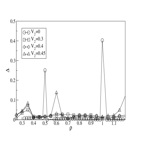
Figure 1: Energy gap (${\Delta}$) vs. density ($\rho$) for different values of ${V_{2}}$. The parameters for this figure are ${t_{1}}=0.1$, ${t_{2}}=0.0$, $U=1.0$, ${V_{1}}=0.7$, ${{\delta}_{t}}=0$ and ${{\delta}_{V}}=0$

Fig. 1 shows the variation of $\Delta$ with $\rho$ for different values of $V_{2}$. At ${V_{2}}=0$, we observe two peaks in the gap at the two densities, ${\rho}=0.5$ and $1$ as reported by Batrouni $et.al$ scal . These peaks shift to $\approx$ 0.35 and $\approx$ 0.65 on introducing nonzero $V_{2}$. Position of peaks remains the same for the other nonzero value of $V_{2}$ we have studied. We note from Fig. 1 that the gap occurs only near the two commensurate fillings of 1/3 and 2/3 (when $V_{2}$ is included in the interaction) and disappears for fillings away from these values. This transition from gapped phase to gapless phase is the commensurate to incommensurate transition; the latter is due to the mismatch between the underlying periodic potential of the lattice and periodicity in the occupancy of the lattice.

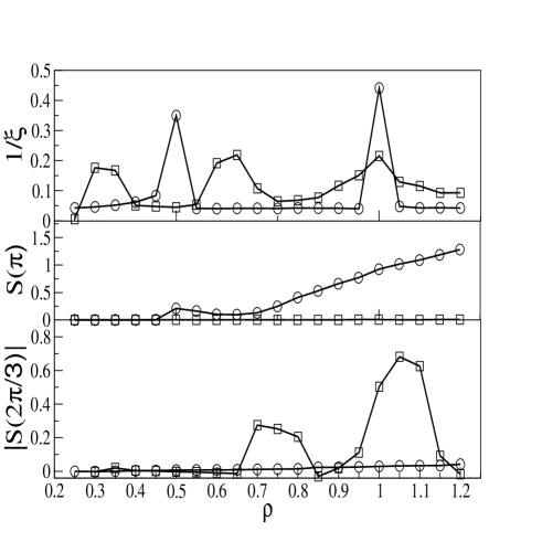
Figure 2: Dependence of inverse correlation length $1/{\xi}$, $S(\pi)$ and $|S(2\pi/3)|$ as a function of ${\rho}$ for $V_{2}=0.0$ and 0.45. Open circle corresponds to $V_{2}=0$ while square corresponds to $V_{2}$=0.45. Other parameter values are $t_{1}=0.1$, $U=1.0$, $V_{1}=0.7$, all other parameters in Eq. 1 are set to zero.

Fig. 2 shows the variation of inverse correlation length of the density-density correlation functions $1/{\xi}$, as well as the structure factor $S(q)$ computed for $q=\pi$ and $2\pi/3$ as a function of boson density, $\rho$, for two different $V_{2}$ values, namely $V_{2}=0$ and $V_{2}=0.45$. We first discuss the ${V_{2}}=0$ case. We note that for $V_{2}=0$, the inverse correlation length shows a peak at $\rho=0.5$ and 1.0 at which values we also note a gap in the system (Fig. 1). The underlying periodicity in the charge density at these $\rho$ values corresponds to dimerization as seen from large $S(\pi)$ at these fillings. We also note that for $V_{2}\neq 0$, the system has vanishing $S(\pi)$ at all fillings. When $V_{2}$ is switched on, the peaks in inverse correlation length shift to $\rho=1/3$ and $\rho=2/3$; at these values we also observe a nonzero gap (Fig.1) in the systems. The underlying charge order corresponds to a periodicity of three lattice sites for $\rho=2/3$, as seen from the peak in $|S(2\pi/3)|$. We also note that $|S(2\pi/3)|$ is vanishingly small for all $\rho$ in the case of $V_{2}=0$. These results are also in broad agreement with field theoretic results.

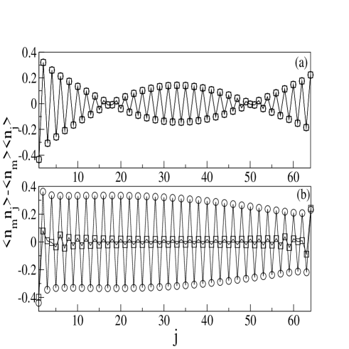
Figure 3: Variation of density-density correlation with distance. (a) one less boson than half-filling, (b) one more boson than half-filling. Squares and circles represent $V_{2}=0$ and $V_{2}=0.3$ respectively.

The charge charge correlation function in the gs for hole -doping and particle doping are shown Figs. 3a and 3b respectively. We note that for the case of hole doping, the ’defect’ brakes up into two solitonic states each with charge half, for both values of $V_{2}$ (0.1 and 0.3) for $U=1$ and $V_{1}=0.7$. However, in case of the particle doping, we note that the two cases have quite different behavior. For $V_{2}=0.1$ we note that the charge-charge correlation function oscillates over the entire chain length. In case of $V_{2}=0.3$, the oscillations are damped in the middle of the chain and become slightly more pronounced at the ends. This behavior is akin to what is seen in the hole-doping case.

Physical picture for this behavior, can be arrived at from an analysis of the $t=0$ Hamiltonian. We find that at $\rho=0.5$ the lowest energy configuration is the one in which alternate site are occupied by a single boson (Fig. 4a top row). On doping with a single hole we find that the energy reduces by $2V_{2}$ (Fig. 4a middle row). However, if the state with these consecutive holes is delocalized (Fig. 4a bottom row) then there is a further stabilization by $V_{2}$. Thus the system prefers to break-up into two defects, with each defect corresponding to two consecutive hole sites. We can formally associate a charge half with each defect since two defects have been created by a single hole doping.

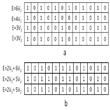
Figure 4: Schematic diagrams of different configurations of half filled bosonic chains with one extra particle and one extra hole together with their energies in the $t_{1}=t_{2}=0$ limit. Panel (a) represents half-filling system with one extra hole whereas panel (b) is for one extra particle.

The case of particle-doping is slightly different. When an empty site is doped (Fig. 4b topline) then the energy increase is $2V_{1}$. Delocalization of the particle, leads to a state with energy $2V_{1}-V_{2}$ ( Fig. 4b middle line), which is stabilized by $V_{2}$ as in the hole-doped case. However, we can also dope a particle at a site which is already occupied by a boson. The energy increase corresponds to $U+2V_{2}$ in this case. Thus, we should observe a 3 consecutive particle state yielding a state with two separated consecutive particle state ( Fig. 4b middle row) only for $2V_{1}<U+2V_{2}$. This is exactly what we find in Fig. 4b. We can identify the ground state for $2V_{1}>U+2V_{2}$ as a Mott insulator state while that for $2V_{1}<U+2V_{2}$ corresponds to a solitonic state.

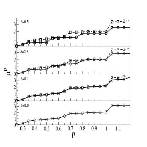
Figure 5: Density ($\rho$) vs. chemical potential ($\mu$) plot. Solid curve with circles are for nonzero dimerization in $t_{1}$ and dashed curves with squares are for nonzero dimerization in $V_{1}$. Parameters space for this figure are ${t_{1}}=0.1$, ${t_{2}}=0.0$, $U=1.0$, ${V_{1}}=0.7$, ${V_{2}}=0.45$.

We now turn our attention to the effect of dimerization on the phase diagrams. We do not assume simultaneous dimerizations in both $V_{1}$ and $t_{1}$ as we wish to explore the role of each of these parameters independently. The effect of dimerization in $t_{1}$ appears to smoothen the $\rho$ vs. $\mu$ behavior. However, the dimerization in $V_{1}$ seems to lead to higher jumps between plateaus, besides changing the value of $\rho$ at which the plateaus occur. It is easy to construct a real space picture for the observed $\rho$ vs $\mu$ behavior if we treat the transfer term as perturbation. In a model with next nearest neighbor interaction in the $t_{1}=0$ limit, it is possible to have a ground state with zero energy for all fillings, $\rho<1/3$ for which the particle can be so distributed that the inter particle interaction in Eq. 1 is zero. At, $\rho=1/3$, when an extra particle is added, there is jump in the gs energy by $(2V_{2})$ which is reflected as a step in the $\rho$ vs. $\mu$ plot. Further addition of particle will increase the gs energy by same amount until $\rho<1/2$, keeping $\mu$ constant between $\rho=1/3$ and $\rho=1/2$. This picture can be extended further for higher fillings. The effect of the transfer term is to reduce the sharpness of the jumps as well as introduce a slow variation in $\mu$ between jumps. For $\rho>1/2$, the chemical potential is nearly $U$ for $U<2V_{1}$ and $2V_{1}$ for $U>2V_{1}$, when transfer term is switched on. Dimerization of the lattice does not significantly affect the $\rho$ vs. $\mu$ behavior at least up to $\rho=1$. Beyond $\rho=1$, the analysis is not straightforward due to the large number of occupancy possibilities afforded by the the bosonic system.

The physics of our system is similar to that of a sawtooth spin chain under a magnetic field mentioned in sec. II. Here $\rho$ of the bosonic model is replaced by the magnetization and $\mu$ is replaced by the magnetic field. We would like to give the physical explanation of the plateau state following the reference hone . The energy levels of a magnetic chain can be labeled by the $M_{s}$ value of the state. When an external magnetic field $H$ is applied the state is stabilized by an energy $-gHM_{s}$. Thus if the $M_{s}$ value of the gs in the absence of an external field is zero, when the field is turned on, the gs switches progressively to higher values of $M_{s}$. If to begin with, the system had gaps between the lowest energy state in different $M_{s}$ sectors, then the $M_{s}$ value of the gs state shows jumps at discrete values of the magnetic field. This results in plateau in the $M_{s}$ vs $H$ plot.

In summary, We have carried out quantum phase analysis of dimerized Bose-Hubbard model, emphasing quantum field theoretic treatment as well as DMRG method to follow the quantum phases. A real space picture of the system in the zero hopping limit gives clear insights into the nature of the quantum phases, which are also predicted by the quantum field in the strongly interacting limit.

Acknowledgement: MK thanks UGC, India for financial support, SS thanks dept. of Physics, IISc for facilities extended. This work was supported in part by a grant from DST (No.SR/S2/CMP-24/2003), India.

References

- (1) O. Penrose and L. Onsager, Phys. Rev. 104, 576 (1956).
- (2) E. Kim and M. H. W. Chan, Nature 427, 225 (2004); Science 305, 1941 (2004).
- (3) A. S. C. Rittner and J. D. Reppy, cond-mat/0604528; J. Day and J. Beamish, Phys. Rev. Lett 96, 105304 (2006).
- (4) B. K. Clark and D. M. Ceperly, Phys. Rev. Lett 96, 105302 (2006); E. Burovski , Phys. Rev. Lett 94, 165301 (2005); M. Boninsegni , Phys. Rev. Lett. 97, 080401 (2006).
- (5) Jaeger, H. M., Haviland, D. B. , Orr, B. G. and Goldmann A. M., Phys. Rev. B 40, 182 (1989),182.
- (6) van der Zant H. S. J. , Fritschy F. C. , Elion W. J. , Geerligs L. J. , and Mooij J. E. , Phys. Rev. Lett, 69, (1992), 2971.
- (7) Chen C. D. , Delsing P. , Haviland D. B. , Harada Y. , and Claeson T. , Phys. Rev. B 51, (1995), 15645.
- (8) Chow E., Delsing P., and Haviland D. B. , Phys. Rev. Lett. 81, (1998), 204.
- (9) F. Dalfovo, S. Giorgini, L. Pitaevskii and S. Stringari, Rev. Mod. Phys 71, 463 (1999).
- (10) A. Leggett, Rev. Mod. Phys 73, 307 (2001).
- (11) L. Pitaevskii, S. Stringari, Bose-Einstein Condensation, Oxford University Press, Oxford 2003.
- (12) C. Pethiek, H. Smith, Bose-Einstein Condensation in Dilute Gases, Cambridge University Press, Cambridge, 2001.
- (13) D. Jaksch, C. Bruder, J. Cirac, C. Gardiner and P. Zoller, Phys. Rev. Lett 81, 3108 (1998).
- (14) D. Jaksch and P. Zoller, Annal of Physics 315, 52 (2005).
- (15) M. Greiner, O. Mandel, T. Esslinger, T. Hansch and I. Bloch, Nature 415, 39 (2002).
- (16) A. Kuklov, N. Prokofev and B. Svistunov, Phys. Rev. Lett 92, 050402 (2004).
- (17) A. Sorensen and K. Molmer, Phys. Rev. Lett 83, 2274 (1999).
- (18) J. K. Pachos and M. B. Plenio, Phys. Rev. Lett 93, 056402 (2004).
- (19) R. Roth and K. Burnett, Phys. Rev. A 69, 021601 (2004).
- (20) M. Lewenstein, L. Santos, M. Baranov, H. Fehrmann, Phys. Rev. Lett 92, 050401 (2004).
- (21) M.P.A. Fisher, P.B. Weichman , G. Grinstein , and D.S. Fisher , Phys. Rev. B 40, 546, (1989).
- (22) D. Kühner Till, S. R. White, and H. Monien, Phys. Rev. B 61, 12474, (2000).
- (23) G. G. Batrouni, F. Hébert , and R. T. Scalettar, Phys. Rev. Lett. 97, 087209, (2006).
- (24) S. R. White , Phys. Rev. Lett. 69 , 2863, (1992).
- (25) R. Pai, R. Pandit, H.R. Krishnamurthy and S. Ramasesha, Phys. Rev. Lett.,Vol. 76, 2937 (1996); R.V. Pai and R. Pandit, Physical Review B, Vol.71, 104508 (2005).
- (26) L. I. Glazmann and A. I. Larkin , Phys. Rev. Lett. 79, 3786, (1997) and references therein.
- (27) R. Fazio , and H. van der Zant, Physics Report 355, 235, (2001).
- (28) T. Giamarchi in Quantum Physics in One Dimension (Claredon Press, Oxford 2004).
- (29) D. Sen, B. S. Shastry, R. E. Walstedt and R. Cava, Phys. Rev. B, 53, 6401, (1996); S. Sarkar and D. Sen, Phys. Rev. B, 65, 172408 ,(2002); Manoranjan Kumar, S. Ramasesha, Diptiman Sen, and Z. G. Soos, Phys. Rev. B, 75 052404 (2007).
- (30) T. Giamarchi, Phys. Rev. B 46, 342 (1992).
- (31) T. Giamarchi, Physica B 230, 975 (1997).
- (32) J. Richter, O. Derzhko and A. Honecker, Cond-Mat/0806.0922.