Renormalization Group Equation and QCD Coupling Constant in the Presence of SU(3) Chromo-Electric Field

Abstract

We solve renormalization group equation in QCD in the presence of SU(3) constant chromo-electric field $E^{a}$ with arbitrary color index $a$=1,2,…8 and find that the QCD coupling constant $\alpha_{s}$ depends on two independent casimir/gauge invariants $C_{1}=[E^{a}E^{a}]$ and $C_{2}=[d_{abc}E^{a}E^{b}E^{c}]^{2}$ instead of one gauge invariant $C_{1}=[E^{a}E^{a}]$. The $\beta$ function is derived from the one-loop effective action. This coupling constant may be useful to study hadron formation from color flux tubes/strings at high energy colliders and to study quark-gluon plasma formation at RHIC and LHC.

I Introduction

Although quantum chromodynamics describes the interaction among quarks and gluons, the classical color field is used in many experimental situations, especially to model the non-perturbative physics. Quark and gluon production from strong chromo-electric field via Schwinger mechanism peter ; schw ; he ; cash itself is a non-perturbative effect. This mechanism is often used in PYTHIA generator pythia to study low $p_{T}$ hadron production at collider experiments. At RHIC and LHC heavy-ion colliders the classical color field play an important role to study production of quark-gluon plasma qgp1 . Color glass condensate provide a natural framework to determine the initial condition on the classical color field at RHIC and LHC larry .

In these situations it is necessary to know how QCD coupling constant depends on SU(3) color field. In this paper we solve the renormalization group equation in QCD in the presence of SU(3) constant chromo-electric field $E^{a}$ with arbitrary color index $a$=1,2,…8. Using background field method in QCD we derive $\beta$ function from the one loop effective action of quark and gluon in the presence of constant chromo-electric field $E^{a}$. Using these two facts we determine the exact dependence of the QCD coupling constant $\alpha_{s}$ on chromo-electric field $E^{a}$ in SU(3).

The paper is organized as follows. In section II we solve renormalization group equation in QCD in the presence of SU(3) chromo-electric field. In section III we derive $\beta$ function from one-loop effective action. In section IV we discuss the dependence of QCD coupling constant on the second casimir invariant in SU(3). We present our conclusions in section V.

II Renormalization Group Equation in QCD in SU(3) Chromo-Electric Field

In the background field method of QCD thooft ; abbott the total gauge field is the sum of classical background field $A_{\mu}^{a}$ and quantum gluon field $Q_{\mu}^{a}$. The gauge fixing term depends on the background field $A_{\mu}^{a}$. As pointed out in abbott it is not necessary to renormalize the quantum gluon fields $Q_{\mu}^{a}$ and the ghost fields. Gauge fixing parameter renormalization is also not necessary because the physical result is gauge fixing parameter independent. Hence the background field $A_{\mu}^{a}$ and coupling constant $g$ need to be renormalized. We define the bare quantities in terms of the renormalized one as follows abbott

$$A_{\mu}^{a}=Z_{A}^{-\frac{1}{2}}~{}A_{\mu r}^{a},~{}~{}~{}~{}~{}~{}~{}~{}~{}~{}~{}~{}~{}g=Z_{g}~{}g_{r}.$$ (1)

This gives

$$F_{\mu\nu}^{a}[A]=Z_{A}^{-\frac{1}{2}}[\partial_{\mu}A_{\nu r}^{a}-\partial_{\nu}A_{\mu r}^{a}+Z_{A}^{-{\frac{1}{2}}}Z_{g}~{}gf^{abc}~{}A_{\mu r}^{b}~{}A_{\nu r}^{c}].$$ (2)

Since $F_{\mu\nu}^{a}[A]$ transforms covariantly with respect to gauge transformation we find from the above equation

$$Z_{g}=Z_{A}^{\frac{1}{2}},~{}~{}~{}~{}~{}~{}~{}~{}~{}~{}~{}~{}~{}{\rm which~{}~{}gives},~{}~{}~{}~{}~{}~{}~{}~{}~{}~{}~{}~{}~{}\beta=-g\gamma,$$ (3)

where we have used

$$\beta=-g\mu\frac{\partial}{\partial\mu}{\rm Ln}Z_{g},~{}~{}~{}~{}~{}~{}~{}~{}~{}~{}~{}~{}~{}~{}{\rm and}~{}~{}~{}~{}~{}~{}~{}~{}~{}~{}~{}~{}~{}\gamma=\frac{1}{2}\mu\frac{\partial}{\partial\mu}{\rm Ln}Z_{A}.$$ (4)

The renormalization group equation for the effective action $\Gamma$ can be written as weinberg

$$[\mu^{2}\frac{\partial}{\partial\mu^{2}}+\beta\frac{\partial}{\partial g}+\gamma\int d^{4}xA^{a}_{\mu}\frac{\delta}{\delta A^{a}_{\mu}}]\Gamma=0.$$ (5)

The effective action may be written in terms of the 1PI Green’s function via

$$\Gamma=\sum_{n}\frac{1}{n!}\int d^{4}x_{1}.....d^{4}x_{n}{\Gamma^{(n)}}^{a_{1},....,a_{n}}_{\mu_{1},....\mu_{n}}(x_{1},...x_{n})A_{\mu_{1}}^{a_{1}}......A_{\mu_{n}}^{a_{n}}.$$ (6)

Using eq. (6) in (5) we find

$$[\mu^{2}\frac{\partial}{\partial\mu^{2}}+\beta\frac{\partial}{\partial g}+n\gamma]\Gamma^{(n)}=0$$ (7)

which is the familiar form of the renormalization group equation in QCD muta .

There is another way to expand the effective action schw ; weinberg . Instead of expanding in powers of $A_{\mu}^{a}$ one can expand in powers of momentum. In coordinate space it has the form

$$\Gamma=\int d^{4}x{\cal L}=\int d^{4}x~{}[-V(A)+\frac{1}{2}(\partial_{\mu}A_{\nu}^{a})^{2}Z_{A}+....].$$ (8)

Hence we will use eq. (5) instead of (7) for the differential equation of the renormalization group. In the presence of constant chromo-electric field the one loop effective action for gluon

$${\cal L}^{(1)}=\sum_{j=1}^{3}{\cal L}^{(1)}_{j}$$ (9)

depends on three independent gauge and Lorentz invariant eigenvalues $\lambda_{j}$ of $f^{abc}E^{c}$ in SU(3)

$$\lambda_{1}^{2}=\frac{C_{1}}{2}[1-{\rm cos}\theta],~{}~{}~{}~{}~{}~{}~{}~{}\lambda_{2,3}^{2}=\frac{C_{1}}{2}[1+{\rm cos}(\frac{\pi}{3}\pm\theta)],~{}~{}~{}~{}~{}~{}~{}~{}{\rm cos}3\theta=-1+\frac{6C_{2}}{C_{1}^{3}}.$$ (10)

Hence the renormalized effective lagrangian density ${\cal L}_{j}$ depends on $\lambda_{j}$. In terms of gauge and Lorentz invariant variables, the renormalization group equation becomes

$$[\mu^{2}\frac{\partial}{\partial\mu^{2}}+\beta\frac{\partial}{\partial g}+\gamma\lambda_{j}\frac{\partial}{\partial\lambda_{j}}]{\cal L}_{j}=0.$$ (11)

In order to solve this differential equation we define dimensionless Lagrangian density

$${\bar{\cal L}_{j}}=\frac{{{\cal L}_{j}}}{\frac{1}{3}\lambda_{j}^{2}}$$ (12)

which can only depend on the dimensionless quantity

$$t_{j}={\rm ln}~{}r_{j}={\rm ln}~{}\frac{g\lambda_{j}}{\mu^{2}}.$$ (13)

We find from eq. (11)

$$\frac{1}{{\bar{\cal L}_{j}}(t_{j})}\frac{\partial{\bar{\cal L}_{j}}(t_{j})}{\partial t_{j}}+\frac{{\bar{\beta}}}{{\bar{\cal L}_{j}}(t_{j})}\frac{\partial{\bar{\cal L}_{j}}(t_{j},g)}{\partial g}=-2{\bar{\gamma}}$$ (14)

where

$${\bar{\beta}}=\frac{\beta}{(\gamma-1)},~{}~{}~{}~{}~{}~{}~{}~{}~{}~{}{\rm and}~{}~{}~{}~{}~{}~{}~{}~{}~{}~{}~{}~{}~{}{\bar{\gamma}}=\frac{\gamma}{(\gamma-1)}.$$ (15)

Solving the differential eq. (14) we find:

$${-\bar{\cal L}_{j}}(t_{j})~{}dt_{j}=-\frac{{\bar{\cal L}_{j}}(t_{j})}{\bar{\beta}}~{}dg=\frac{d{{\bar{\cal L}_{j}}(t_{j})}}{2{\bar{\gamma}}}$$ (16)

which gives

$$\frac{dg}{dt_{j}}={\bar{\beta}}.$$ (17)

In this paper we consider $\alpha_{s}$ at the one loop level and take the $\beta$ function of the form

$${\bar{\beta}}(g)=-{\bar{\beta}_{0}}g^{3}.$$ (18)

We find from eq. (17) the QCD coupling constant

$$\alpha_{s}(\lambda_{j})=\frac{g^{2}(t_{j})}{4\pi}=\frac{g^{2}}{4\pi[1+2{\bar{\beta}_{0}}g^{2}t_{j}]}=\frac{\alpha_{s}}{[1+4\pi{\bar{\beta}_{0}}\alpha_{s}{\rm Log}(\frac{g^{2}\lambda_{j}^{2}}{\mu^{4}})]}=\frac{1}{4\pi{\bar{\beta}_{0}}{\rm Log}(\frac{g^{2}\lambda_{j}^{2}}{\Lambda^{4}})}$$ (19)

where

$$\Lambda=\mu~{}e^{(-1/(4{\bar{\beta}_{0}}g^{2}))},~{}~{}~{}~{}~{}~{}~{}~{}~{}~{}~{}~{}~{}~{}~{}~{}\alpha_{s}=\frac{g^{2}}{4\pi}.$$ (20)

For the quark case the $\beta$ functions are different and the eigenvalues are in fundamental representation of SU(3). Three independent gauge and Lorentz invariant eigenvalues of $T^{a}_{ij}E^{a}$ for the quark case are given by

$$\lambda_{1}=\sqrt{\frac{C_{1}}{3}}{\rm cos}\theta,~{}~{}~{}~{}~{}~{}~{}~{}\lambda_{2,3}=\sqrt{\frac{C_{1}}{3}}{\rm cos}(\frac{2\pi}{3}\pm\theta),~{}~{}~{}~{}~{}~{}~{}~{}{\rm cos}^{2}3\theta=\frac{3C_{2}}{C_{1}^{3}}.$$ (21)

All now remains is to find the $\beta$ functions from one-loop effective action which we will derive in the next section.

III $\beta$ function in QCD from one-loop effective action

The one-loop effective lagrangian density for gluon in the presence of SU(3) constant chromo-electric field $E^{a}$ with $a$=1,2,…8 is given by peter

$${\cal L}^{(1)}_{j}=\frac{1}{8\pi^{2}}\int_{0}^{\infty}\frac{ds}{s^{2}}[g\lambda_{j}\frac{{\rm cos}2g\lambda_{j}s}{{\rm sin}g\lambda_{j}s}-\frac{1}{s}].$$ (22)

Expanding ${\rm sin}$ and ${\rm cos}$ functions we get

$${\cal L}^{(1)}_{j}=\frac{1}{8\pi^{2}}\int_{0}^{\infty}\frac{ds}{s^{2}}[-\frac{11g^{2}\lambda_{j}^{2}s}{6}+\frac{39g^{4}\lambda_{j}^{4}}{240}s^{3}+...].$$ (23)

Since $s$ has dimension of length, the ultra violate divergence occurs at $s\rightarrow 0$ which leads to charge renormalization schw . The ultra violate divergent term in eq. (23) is $\frac{1}{8\pi^{2}}\int_{0}^{\infty}\frac{ds}{s}\frac{11g^{2}\lambda_{j}^{2}}{6}$. We write eq. (22) as follows

$${\cal L}^{(1)}_{j}=\frac{1}{8\pi^{2}}\int_{0}^{\infty}\frac{ds}{s^{2}}[g\lambda_{j}\frac{{\rm cos}2g\lambda_{j}s}{{\rm sin}g\lambda_{j}s}+\frac{11g^{2}\lambda_{j}^{2}s}{6}-\frac{1}{s}]-\frac{1}{8\pi^{2}}\int_{0}^{\infty}\frac{ds}{s}\frac{11g^{2}\lambda_{j}^{2}}{6}.$$ (24)

The $s$ integration involving the square bracket term is now finite. We can obtain the $\beta$ function from the coefficient of the divergent term by renormalization procedure by adding the counter term $Z{\cal L}_{0}$. We put a cut-off for the infrared limit at $s=s_{0}$ and by change to the dimensionless variable $s_{j}\rightarrow sg\lambda_{j}$. We find

$${\cal L}^{(1)}_{j}=\frac{g^{2}\lambda_{j}^{2}}{8\pi^{2}}\int_{0}^{\infty}\frac{ds_{j}}{s_{j}^{2}}[\frac{{\rm cos}2s_{j}}{{\rm sin}s_{j}}+\frac{11}{6}-\frac{1}{s_{j}}]-\frac{1}{8\pi^{2}}\int_{0}^{g\lambda_{j}s_{0}}\frac{ds_{j}}{s_{j}}\frac{11g^{2}\lambda_{j}^{2}}{6}.$$ (25)

The free lagrangian density is given by

$${\cal L}_{0}=\frac{E^{a}E^{a}}{2}=\frac{1}{3}\sum_{j=1}^{3}\lambda_{j}^{2}~{}=~{}\sum_{j=1}^{3}{\cal L}_{0}^{j}.$$ (26)

Adding the counter term ($Z{\cal L}_{0}^{j}$) to eq. (25) the renormalized lagrangian density becomes

$${\cal L}_{j}(t_{j})=Z{\cal L}_{0}^{j}+{\cal L}^{(1)}_{j}.$$ (27)

The renormalization condition is then given by

$$\frac{{\cal L}_{j}(t_{j})}{{\cal L}_{0}^{j}}|_{t_{j}=0}=1.$$ (28)

We find from the above equation

$$Z=1-3\frac{g^{2}}{8\pi^{2}}\int_{0}^{\infty}\frac{ds_{j}}{s_{j}^{2}}[\frac{{\rm cos}2s_{j}}{{\rm sin}s_{j}}+\frac{11}{6}-\frac{1}{s_{j}}]+\frac{3}{8\pi^{2}}\int_{0}^{g\mu^{2}s_{0}}\frac{ds_{j}}{s_{j}}\frac{11g^{2}}{6}$$ (29)

which when used in eq. (27) gives the renormalized Lagrangian density

$${\bar{\cal L}}_{j}=\frac{{\cal L}_{j}(t_{j})}{{\cal L}_{0}^{j}}=1-\frac{11}{16\pi^{2}}g^{2}t_{j}.$$ (30)

The $\beta$ function can be obtained from the renormalized Lagrangian density. From eqs. (14), (12) and (28) we find

$${\bar{\gamma}}=-\frac{1}{2}\frac{\partial{{\bar{\cal L}}_{j}}(t_{j})}{\partial t_{j}}|_{t_{j}=0}.$$ (31)

Using eqs. (15) and (3) in the above equation we find

$${\bar{\beta}}=\frac{g}{2}~{}\frac{\partial{{\bar{\cal L}}_{j}}(t_{j})}{\partial t_{j}}|_{t_{j}=0}.$$ (32)

Using eq. (32) we find from eq. (30)

$${\bar{\beta}}=-\frac{11}{32\pi^{2}}g^{3}$$ (33)

which gives the $\beta$ function for a gluon loop

$${\bar{\beta_{0}}}^{g}=\frac{11}{32\pi^{2}}$$ (34)

where we have used eq. (18).

The effective Lagrangian density for massless quark is given by peter

$${\cal L}^{(1)}_{j}=-\frac{1}{8\pi^{2}}\int_{0}^{\infty}\frac{ds}{s^{2}}[g\lambda_{j}\frac{{\rm cos}g\lambda_{j}s}{{\rm sin}g\lambda_{j}s}-\frac{1}{s}].$$ (35)

Expanding ${\rm sin}$ and ${\rm cos}$ functions we get

$${\cal L}^{(1)}=-\frac{1}{8\pi^{2}}\int_{0}^{\infty}\frac{ds}{s}[\frac{g^{2}\lambda_{j}^{2}}{3}+\frac{g^{4}\lambda_{j}^{4}}{20}s^{2}+...].$$ (36)

The coefficient of the ultra violate divergent term (as $s\rightarrow 0$) is $\frac{1}{3}$. The free Lagrangian density is given by

$${\cal L}_{0}=\frac{E^{a}E^{a}}{2}=\sum_{j=1}^{3}\lambda_{j}^{2}~{}=~{}\sum_{j=1}^{3}{\cal L}_{0}^{j}.$$ (37)

Carrying out similar renormalization analysis as for gluons we obtain the renormalized Lagrangian density

$${\bar{\cal L}}_{j}=1+\frac{1}{24\pi^{2}}g^{2}t_{j}$$ (38)

which gives the $\beta$ function for a quark loop

$${\bar{\beta_{0}}}^{q}=-\frac{1}{48\pi^{2}}.$$ (39)

To summarize, eq. (19) describes evolution of QCD coupling constant in the presence of SU(3) constant chromo-electric field, together with eqs. (34) and (39) as ${\bar{\beta}}_{0}$ functions for a gluon and quark loop respectively.

IV QCD Coupling Constant and Second Casimir Invariant in SU(3)

It can be seen that the two independent casimir invariants $C_{1}=[E^{a}E^{a}]$ and $C_{2}=[d_{abc}E^{a}E^{b}E^{c}]^{2}$ in SU(3) are gauge invariant with respect to the gauge transformation

$$(T^{a}E^{a})^{\prime}=U(T^{a}U^{a})U^{-1},~{}~{}~{}~{}~{}~{}~{}~{}~{}~{}~{}~{}~{}~{}~{}~{}U=e^{iT^{a}\omega^{a}(x)}.$$ (40)

Let us denote the vector ${\vec{E}}$ in 8-dimensional color space in SU(3) with components $E_{a}=(E_{1},~{}E_{2},~{}.....,E_{8})$. It can be seen that while the first casimir invariant $C_{1}$ is independent of the direction of the vector ${\vec{E}}$, the second casimir invariant $C_{2}$ may depend on the direction of ${\vec{E}}$ in 8-dimensional color space even if it is gauge invariant. This is because of presence of $d_{abc}$ whose components are not equal to each other pdg . These two independent casimir invariants satisfy the limit

$$0\leq\frac{3C_{2}}{C_{1}^{3}}\leq 1.$$ (41)

Eq. (41) gives the limit

$$0\leq\theta\leq\frac{2\pi}{3}$$ (42)

when the $\lambda_{j}$’s are given by eq. (10) in the adjoint representation of SU(3) and

$$\frac{\pi}{6}\leq\theta\leq\frac{\pi}{2}$$ (43)

when the $\lambda_{j}$’s are given by eq. (21) in the fundamental representation of SU(3).

Since $\theta$ appears inside $log$ in $\alpha_{s}(\lambda_{j})$ it is useful to check that this $\theta$ dependence is under control for this one loop calculation. When the $\lambda_{j}$’s are given by eq. (10), it can be checked that the one-loop result of $\alpha_{s}(\lambda_{j})$ in the maximum allowed range $0\leq\theta\leq\frac{2\pi}{3}$ (see eq. (42)) is under control only for asymptotically very large value of $C_{1}=[E^{a}E^{a}]$ (see below). Similarly, when the $\lambda_{j}$’s are given by eq. (21), the one-loop result of $\alpha_{s}(\lambda_{j})$ in the maximum allowed range $\frac{\pi}{6}\leq\theta\leq\frac{\pi}{2}$ (see eq. (43)) is under control only for asymptotically very large value of $C_{1}=[E^{a}E^{a}]$.

For realistic values of $C_{1}=[E^{a}E^{a}]$, $g$ and $\Lambda$ at RHIC and LHC we can determine the range of $\theta$ for which $0<\alpha_{s}\leq 1$ in this one-loop calculation of $\alpha_{s}$. For example, by using eq. (10) we find from $0<\alpha_{s}\leq 1$, the range

$${\rm cos}^{-1}[1~{}-~{}\frac{2\Lambda^{4}}{g^{2}C_{1}}e^{\frac{1}{4\pi{\bar{\beta}_{0}}}}]~{}\leq~{}\theta~{}\leq~{}-\pi/3~{}+~{}{\rm cos}^{-1}[\frac{2\Lambda^{4}}{g^{2}C_{1}}e^{\frac{1}{4\pi{\bar{\beta}_{0}}}}~{}-~{}1].$$ (44)

It can be seen that when $C_{1}=[E^{a}E^{a}]$ is asymptotically very large, say, $C_{1}\rightarrow\infty$ we find from eq. (44), $0\leq\theta\leq\frac{2\pi}{3}$ which reproduces the maximum allowed range as given by eq. (42). For realistic values of $C_{1}=[E^{a}E^{a}]$, $g$ and $\Lambda$ at RHIC and LHC the range in eq. (44) may be be very close to the maximum allowed range in eq. (42). For example, if we choose $\Lambda$=0.2 GeV, g=3 and $C_{1}=E^{a}E^{a}$ = 1000 GeV⁴ (which may be a reasonable value at LHC) we find from eq. (44), $0.0021\leq\theta\leq 2.092$. This range of $\theta$ is very close to the maximum allowed range $0\leq\theta\leq\frac{2\pi}{3}$ or $0\leq\theta\leq 2.094$ as given by eq. (42).

Similarly, by using eq. (21) we find from $0<\alpha_{s}\leq 1$, the range

$$\frac{2\pi}{3}-{\rm cos}^{-1}[\sqrt{\frac{3\Lambda^{4}}{g^{2}C_{1}}e^{\frac{1}{4\pi{\bar{\beta}_{0}}}}}]~{}\leq~{}\theta~{}\leq~{}{\rm cos}^{-1}[\sqrt{\frac{3\Lambda^{4}}{g^{2}C_{1}}e^{\frac{1}{4\pi{\bar{\beta}_{0}}}}}].$$ (45)

It can be seen that when $C_{1}=[E^{a}E^{a}]$ is asymptotically very large, say, $C_{1}\rightarrow\infty$ we find from eq. (45), $\frac{\pi}{6}\leq\theta\leq\frac{\pi}{2}$ which reproduces the maximum allowed range as given by eq. (43). If we choose the previous values, $\Lambda$=0.2 GeV, g=3 and $C_{1}=E^{a}E^{a}$ = 1000 GeV⁴ we find from eq. (45), $0.526\leq\theta\leq 1.569$. This range of $\theta$ is very close to the maximum allowed range $\frac{\pi}{6}\leq\theta\leq\frac{\pi}{2}$ or $0.5236\leq\theta\leq 1.571$ as given by eq. (43).

In Fig. 1 we present the result of $\alpha_{s}(\lambda_{j})$ as function of $\theta$ for fixed values of $C_{1}=[E_{a}E_{a}]$. We have used $g$=3 and $\Lambda$= 200 MeV. The scale $\lambda_{j}$’s are given by eq. (10). The range of $\theta$ in Fig. 1 is given by eq. (44). The upper, middle and lower solid lines are the results of $\alpha_{s}(\lambda_{1})$ for $C_{1}$ = 10, 1000 and 100000 GeV⁴ respectively. The upper, middle and lower dotted lines are the results of $\alpha_{s}(\lambda_{2})$ for $C_{1}$ = 10, 1000 and 100000 GeV⁴ respectively. The upper, middle and lower dashed lines are the results of $\alpha_{s}(\lambda_{3})$ for $C_{1}$ = 10, 1000 and 100000 GeV⁴ respectively. It can be seen from Fig. 1 that the $\theta$ dependence is under control for the entire range of $\theta$ as given by eq. (44) which is very close to the actual maximum range $0\leq\theta\leq\frac{2\pi}{3}$ in eq. (42).

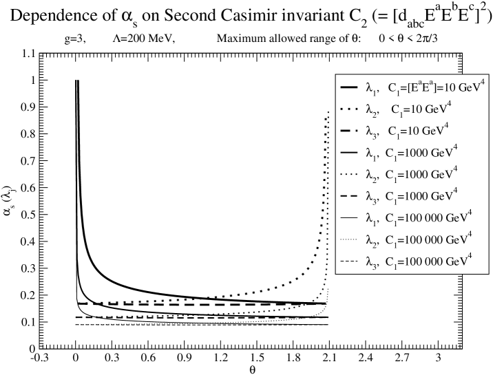
Figure 1: QCD coupling constant in the presence of SU(3) chromo-electric field as function $\theta$ for fixed values of first casimir invariant $C_{1}=E^{a}E^{a}$. The $\lambda_{j}$’s used are from eq. (10). Remember that $0\leq\theta\leq\frac{2\pi}{3}$ is the maximum range when the $\lambda_{j}$’s are given by eq. (10).

In Fig. 2 we present the result of $\alpha_{s}(\lambda_{j})$ as function of $\theta$ for fixed values of $C_{1}=[E_{a}E_{a}]$. We have used $g$=3 and $\Lambda$= 200 MeV. The scale $\lambda_{j}$’s are given by eq. (21). The range of $\theta$ in Fig. 2 is given by eq. (45). The upper, middle and lower solid lines are the results of $\alpha_{s}(\lambda_{1})$ for $C_{1}$ = 10, 1000 and 100000 GeV⁴ respectively. The upper, middle and lower dotted lines are the results of $\alpha_{s}(\lambda_{2})$ for $C_{1}$ = 10, 1000 and 100000 GeV⁴ respectively. The upper, middle and lower dashed lines are the results of $\alpha_{s}(\lambda_{3})$ for $C_{1}$ = 10, 1000 and 100000 GeV⁴ respectively. It can be seen from Fig. 2 that the $\theta$ dependence is under control for the entire range of $\theta$ as given by eq. (45) which is very close to the actual maximum range $\frac{\pi}{6}\leq\theta\leq\frac{\pi}{2}$ in eq. (43).

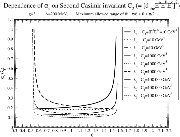
Figure 2: QCD coupling constant in the presence of SU(3) chromo-electric field as function $\theta$ for fixed values of first casimir invariant $C_{1}=E^{a}E^{a}$.The $\lambda_{j}$’s used are from eq. (21). Remember that $\frac{\pi}{6}\leq\theta\leq\frac{\pi}{2}$ is the maximum range when the $\lambda_{j}$’s are given by eq. (21).

It can be seen from Fig. 1 and Fig. 2 that, for same values of $\theta$, the value of $\alpha_{s}$ decreases as $C_{1}=[E^{a}E^{a}]$ increases which is consistent with asymptotic freedom.

In Fig. 3 we present the result of $\alpha_{s}(\lambda_{j})$ as function of $C_{1}=[E_{a}E_{a}]$ for fixed values of $\theta$. We have used $g$=3 and $\Lambda$= 200 MeV. The scale $\lambda_{j}$’s are given by eq. (10). The solid line is the result of $\alpha_{s}(\lambda_{1})$ for $\theta~{}=~{}\frac{\pi}{6}$. The dotted line is the result of $\alpha_{s}(\lambda_{2})$ for $\theta~{}=~{}\frac{\pi}{3}$ and the dashed line is the result of $\alpha_{s}(\lambda_{3})$ for $\theta~{}=~{}\frac{\pi}{2}$. In this figure we have chosen three different values of $\theta$ which are within the maximum allowed range $0\leq\theta\leq\frac{2\pi}{3}$ as given by eq. (42). It can be seen from Fig. 3 that the $\theta$ dependence is under control in the entire range of $C_{1}=[E_{a}E_{a}]$.

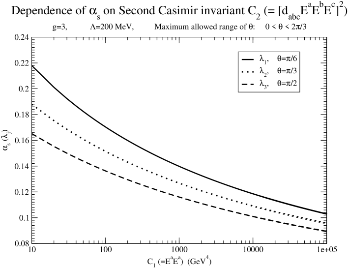
Figure 3: QCD coupling constant in the presence of SU(3) chromo-electric field as function of first casimir invariant $C_{1}=[E^{a}E^{a}]$ for fixed values of $\theta$. The $\lambda_{j}$’s used are from eq. (10). Remember that $0\leq\theta\leq\frac{2\pi}{3}$ is the maximum range when the $\lambda_{j}$’s are given by eq. (10).

In Fig. 4 we present the result of $\alpha_{s}(\lambda_{j})$ as function of $C_{1}=[E_{a}E_{a}]$ for fixed values of $\theta$. We have used $g$=3 and $\Lambda$= 200 MeV. The scale $\lambda_{j}$’s are given by eq. (21). The solid line is the result of $\alpha_{s}(\lambda_{1})$ for $\theta~{}=~{}\frac{5\pi}{12}$. The dotted line is the result of $\alpha_{s}(\lambda_{3})$ for $\theta~{}=~{}\frac{\pi}{3}$ and the dashed line is the result of $\alpha_{s}(\lambda_{2})$ for $\theta~{}=~{}\frac{\pi}{4}$. In this figure we have chosen three different values of $\theta$ which are within the maximum allowed range $\frac{\pi}{6}\leq\theta\leq\frac{\pi}{2}$ as given by eq. (43). It can be seen from Fig. 4 that the $\theta$ dependence is under control in the entire range of $C_{1}=[E_{a}E_{a}]$.

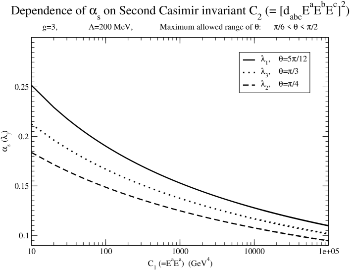
Figure 4: QCD coupling constant in the presence of SU(3) chromo-electric field as function of first casimir invariant $C_{1}=[E^{a}E^{a}]$ for fixed values of $\theta$. The $\lambda_{j}$’s used are from eq. (10). Remember that $\frac{\pi}{6}\leq\theta\leq\frac{\pi}{2}$ is the maximum range when the $\lambda_{j}$’s are given by eq. (21).

It can be seen from Fig. 3 and Fig. 4 that the value of $\alpha_{s}$ decreases as $C_{1}=[E^{a}E^{a}]$ increases which is consistent with asymptotic freedom.

V Conclusion

We have solved renormalization group equation in QCD in the presence of SU(3) constant chromo-electric field $E^{a}$ with arbitrary color index $a$=1,2,…8. Using background field method in QCD we have obtained the $\beta$ function from one loop effective action of quark and gluon in the presence of chromo-electric field $E^{a}$ in SU(3). Using these two facts we have determined the exact dependence of the QCD coupling constant on $E^{a}$. We have found that the renormalization scale of the QCD coupling constant $\alpha_{s}$ depends on two independent casimir/gauge invariants $C_{1}=[E^{a}E^{a}]$ and $C_{2}=[d_{abc}E^{a}E^{b}E^{c}]^{2}$ instead of one gauge invariant $C_{1}=[E^{a}E^{a}]$. These coupling constant may play an important role in the study of production and equilibration of quark-gluon plasma from classical color field at RHIC and LHC. This coupling constant may also play an important role to study low $p_{T}$ hadron production at collider experiments using string breaking mechanism in the color flux-tube model.

References

(1) G. C. Nayak and P. van Nieuwenhuizen,
Phys. Rev. D71 (2005) 125001; F. Cooper and G. C. Nayak, Phys. Rev. D73
(2006) 065005; G. C. Nayak, Phys. Rev. D72 (2005) 125010.
(2) J. Schwinger, Phys. Rev. 82 (1951) 664.
(3) W. Heisenberg and H. Euler, Z. Physik 98, 714 (1936).
(4) A. Casher, H. Neuberger and S. Nussinov, Phys. Rev. D 20, 179 (1979).
(5) B. Andersson, the Lund model, Cambridge University Press,
Cambridge, 1998); PYTHIA: http://www.thep.lu.se/(tilde)torbjorn/pythia.html
(6) F. Cooper, E. Mottola and G. C. Nayak, Phys. Lett. B 555, 181 (2003);
G. C. Nayak et al., Nucl. Phys. A687, 457 (2001).
(7) L. McLerran and R. Venugopalan, Phys. Rev. D49 (1994) 2233; Phys. Rev. D49
(1994) 3352; E. Iancuu, A. Leonidov and L. McLerran, Phys. Lett. B510 (2001) 133;
E. Iancuu, A. Leonidov and L. McLerran, Nucl. Phys. A692 (2001) 583; J. Jalilian-Marian,
A. Kovner, L. Mcerran and H. Weigert, Phys. Rev. D55 (1997) 5414.
(8) G. ’t Hooft, Nucl. Phys. B62 (1973) 444.
(9) L. F. Abbott, Nucl. Phys. B185 (1981) 189.
(10) S. Coleman and E. Weinberg, Phys. Rev. D 7 (1973) 1888.
(11) T. Muta, Foundations of Quantum Chromodynamics,
(World scientific lecture notes in physics-vol. 5).
(12) For a list of non-zero values of , see for example, Particle Data Group, http://pdg.lbl.gov/.