Deformed Gaussian Orthogonal Ensemble description of Small-World networks
Abstract
The study of spectral behavior of networks has gained enthusiasm over the last few years. In particular, Random Matrix Theory (RMT) concepts have proven to be useful. In discussing transition from regular behavior to fully chaotic behavior it has been found that an extrapolation formula of the Brody type can be used. In the present paper we analyze the regular to chaotic behavior of Small World (SW) networks using an extension of the Gaussian Orthogonal Ensemble. This RMT ensemble, coined the Deformed Gaussian Orthogonal Ensemble (DGOE), supplies a natural foundation of the Brody formula. SW networks follow GOE statistics till certain range of eigenvalues correlations depending upon the strength of random connections. We show that for these regimes of SW networks where spectral correlations do not follow GOE beyond certain range, DGOE statistics models the correlations very well. The analysis performed in this paper proves the utility of the DGOE in network physics, as much as it has been useful in other physical systems.
I Introduction
Initiated by two seminal works SW ; BA , the last decade has witnessed a spurt in activities of network research SW ; rev-Strogatz ; rev-network . Regular and random networks are the two limiting cases of network topology. For the regular network, each node is connected in a fixed pattern to the same number of neighboring nodes; on the other hand, for the random network, each node is randomly joined with any other node. Real-world networks show the properties which are intermediate of the regular and the random one SW ; rev-Strogatz ; rev-network . For example, many real-world networks from diverse field have very small diameter but have very high clustering, two characteristics shown respectively by random and regular networks. To model randomness and regularity, Watts and Strogatz proposed an algorithm to generate popularly known as Small-World (SW) network, which has the properties of small diameter and high clustering SW . Moreover, this model network is very sparse, i.e. network with a very few number of edges, which is another property shown by real-world networks.
The structure of networks is described by its associated adjacency matrix . It is defined in the following way: if and nodes are connected and zero otherwise. We consider only undirected networks. In this case, the adjacency matrix is symmetric and consequently has real eigenvalues. These eigenvalues give information about some basic topological properties of the underlying network handbook . The fluctuations of these eigenvalues can be studied by Random Matrix Theory (RMT).
There is a long history of applications of random matrix ensembles to model fluctuations of the spectra of diverse systems guhr . Unfortunately analytical results exist only if some ideal conditions are fulfilled by the systems studied. On the other hand real physical systems usually depart from these conditions. In order to cover these situations other ensembles have been introduced Dyson . One such class of ensemble is the so-called deformed Gaussian orthogonal ensemble (DGOE) dgoe1 ; dgoe2 ; dgoe3 . This ensemble has been proved to be particularly useful when one wants to study the breaking of a discrete symmetry in a many-body system such as the atomic nucleus. It is also useful for studying transition among classes of ensemble such as order-chaos (Poisson GOE) and symmetry violation (2GOE GOE) dgoe4 . Recently Jalan and Bandyopadhyay show that spectra of various model networks and real world networks follow universal random matrix properties SJ_pre2007a ; SJ_pre2007b , intermediate between Poisson and GOE statistics. Correlations among eigenvalues of SW networks follow GOE statistics of RMT for certain range and after that they deviate from the GOE statistics SJ_New . We believe that the DGOE supplies a RMT basis for the Brody Brody distribution and gives a more accurate description of the GOE-Poisson transition than the Berry-Robnik Berry model, which purports to justify the Brody formula from an RMT stand point. The Brody distribution was used previously in SW statistics investigation SJ_pre2007a ; SJ_pre2007b . In the present paper we analyze the spectra of SW model networks using DGOE. Based on the results of reference SJ_New we argue, and show through numerical simulations that fluctuations of the spectra of the SW model follows the description of a transition Poisson-GOE.
II Small-World networks
Watts-Strogatz model of SW network is constructed by rewiring the edges of regular ring lattice with probability . This rewiring procedure generates a network with some random connections, without altering the number of vertices or edges. For , structure of the regular lattice or -nearest neighbor coupled network remains same; on the other hand, for , the regular lattice becomes random network. For the intermediate values of , the graph is a SW network: highly clustered like a regular graph, yet with small characteristic path length like a random graph. This onset of SW property happens for a very small value of parameter . Characteristic path length is defined as the number of connections in the shortest path between two nodes, averaged over all pairs of nodes. For a network of size and average degree , it scales as if network is regular, and if network is random. Clustering coefficient () is defined as the ratio of connections between neighbors to the number of allowed links. For regular graphs is very high (), whereas for random graphs it scales as . Small-world networks show intermediate behavior between these two extremes, with average path length being as low as for the random graphs, and clustering coefficient as high as that of regular graphs. This intermediate statistical features of SW networks are reflected in their spectral fluctuations, and can be nicely described using the DGOE which provides a RMT basis for the deviation from the GOE behavior of the short range correlation aspect of the eigenvalues, exemplified through the spacing distribution, and the long range correlation measured by the . In the following we supply a description of the GOE-Poisson transition within the DGOE.
III The Deformed Gaussian Orthogonal Ensemble (DGOE): Transitions Among Universality Classes in RMT
The joint probability distribution of elements of DGOE has the general form dgoe2
| (1) |
where is a normalization factor and is the trace of the matrix . In order to describe two interpolating ensemble the matrix must be chosen as the sum of two terms
| (2) |
where the matrices and define complementary subspaces of . According to (1) for the elements of vanish and is projected onto the matrix . Since in this work we are concerned with the statistics intermediate between Poisson and GOE we will define as the Poissonian ensemble. It will be a diagonal matrix with elements given by whose eigenvalues are independent random variable with Gaussian distribution
| (3) |
and variance
| (4) |
The elements of the diagonal-less matrix are also random independent variables with zero mean and variance given by
| (5) |
where . When () the ensemble corresponds to the GOE. In the limit , there will be only diagonal elements and the Poisson regime is attained.
The average level density
| (6) |
and the cumulative level density
| (7) |
were calculated by Bertuola et al. dgoe5 , who observed that formula (7) provides a more accurate manner of unfolding the spectra than the usual polynomial unfolding used in ueda . These formulas work very well in the regime close either to Poisson or GOE statistics. Intermediate between these statistics there is a transition regime characterized by a rapid change in statistics from almost Poisson to almost GOE. In this regime formulas (6) and (7) need corrections (see foot ).
IV Simulations and Results
Numerical simulations of the SW networks are made by considering ensembles of 20 networks of size and average degree . The adjacency matrix was diagonalized numerically and its first and last 300 eigenvalues were discarded. Since an analytical expression for the average density is still lacking, the unfolding of eigenvalues was made by fitting the cumulative density or stair-case function
| (8) |
to Chebyshev polynomial using the linear least squares method. are the eigenvalues of the SW network and is the unit step function.
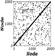
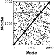
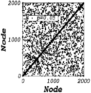
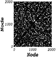
For , the corresponding adjacency matrix would be a banded matrix with entries one in the band. As some connections are randomized with probability , corresponding adjacency matrix gets some non-zero entries outside the band, at the expense of equal numbers of entries of in the band. The mean value of the elements of these matrices is and variance is . Fig. (1)-(6) plot the adjacency matrix for different rewiring probabilities. Left sub-figure of (1) plots the adjacency matrix at the onset of SW transition (). For such a small value of , very few connections are rewired and hence adjacency matrix is still almost banded with very few connections outside the band. Note that we take average degree of network as , which leads to a sparse network (i.e. the number of connections is of the order of the number of nodes). Left sub-figure of Fig. (6) plots the adjacency matrix for , for this value of , 20% of connections are rewired leading to the equal number of outside the band.
Results for the statistics intermediate between Poisson and GOE are obtained by diagonalization of an ensemble of random matrices. The mean value of the elements of these matrices were taken zero and the variance of the diagonal and off-diagonal elements given by (4) and (5). The unfolding of the spectra of the matrices is done using (7). In the simulations the values of and the size of matrices are kept fixed. In order to simulate a transition Poisson-GOE, ensembles with 100 matrices and different values of are considered. For each value of we check between the density of eigenvalue given by (6) and the density of eigenvalues from the numerical calculation. If the agreement between the two is poor, the simulations are re-run using a corrected version of , and (called and A in dgoe5 ) foot . These corrections are needed especially in the transitional regime alluded to following the discussion below Eq. (7).
In the discussion of the deviation of the spacing distribution from that of Wigner, SW practitioners have used the Brody distribution,Brody , which is given by,
| (9) |
where and are related to through the normalization condition. Another distribution which also purports to describe the transition case was derived by Berry using RMT and semiclassical considerations. The DGOE, which we use in this paper, supplies a natural RMT for the description of the GOE-Poisson and/or the Poisson-GOE transitions.
In order to investigate the long-range behavior among the eigenvalues of SW model we use the Dyson-Mehta statistics . It is defined as
| (10) |
where and are obtained from a least-square fit. is the average number of spacings in the integration interval, and the number of eigenvalues which are less than (for DGOE is given by (7) ). measures the least-square deviation of the function (the unfolded spectra) from a straight line in the interval . In order to improve the statistics and avoid the introduction of correlations we choose successive intervals which overlap by boh . According to RMT, for GOE the expected value for large values of approaches
| (11) |
and for Poisson statistics it approaches .
In the following we present results for SW networks for various values, and corresponding DGOE. The nearest neighbor spacing distribution of SW networks, which probes for short range correlations of spectra, for the range of can be modeled by Brody parameter as described in SJ_pre2007a . After this values of , which corresponds to the SW transition as defined by Strogatz-Watts SW , the short range correlations of spectra still follows GOE statistics, but the long range correlations probed via statistics follows GOE statistics only for certain range, and after that deviation from GOE statistics is seen SJ_pre2007b ; SJ_New . Which indicates possible breakdown of GOE theory for SW networks. And hence we turn to the random matrix theory of DGOE. Note that for the range for which follows GOE statistics depends upon the size and average degree of the network as well SJ_New .
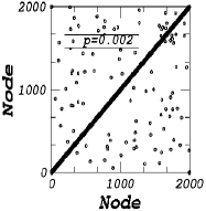
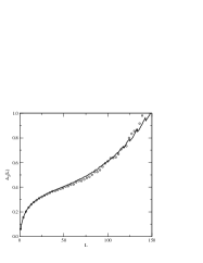
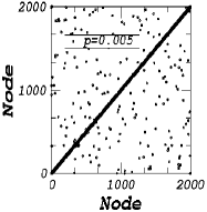
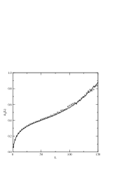


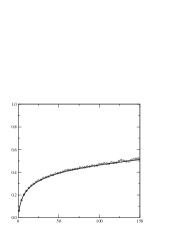

In Figs. (1) to (6), the spectral rigidity are presented for the different values of . The values of varies from , corresponding to the onset of SW behavior, to which corresponds to a random graph. Each figure also depicts the for DGOE describing a transition Poisson-GOE. The DGOE simulations are performed for matrices of size N=2000. Note that for each value of it is possible to find a correspondent such for which DGOE fits for SW model. The values of parameters and are listed in the table 1. Using the criteria developed in entropia we find that the critical value of which separates the chaotic (random) from regular regime is . Therefore before this value of the SW model is still in the regular regime, although the distribution of nearest neighbor spacing is totally compatible with a GOE description. The multi-peaks in the density of eigenvalues for these values of SJ_New ; Farkas also supports this finding, because it indicates that the network still has large amount of regularity. In Fig. (3) to (6) the values for are increased and the comes into the chaotic (random) regime. As the value of increases the spectra of becomes closer to the GOE prediction. In other words, the local regularity is gradually destroyed and the network becomes random. The DGOE description which we are using to model SW to random network behavior, shows that for , behavior of statistics can be modeled by a single value of . It suggests that under the framework of DGOE description, the network with has as much symmetry as for a complete random network ().
V Conclusion and Discussion
According to the RMT the Poisson statistic describes systems with localized states on
certain bases and uncorrelated spectrum. On the other hand the GOE describes systems
that become ergodic in the thermodynamic limit and have correlated spectra.
For we have the ring graph which possesses symmetry (rotational symmetry). The
numerical calculations of the spectra show several degenerate eigenvalues
SJ_New . There is no level repulsion and the spectra of ring graph should
follow the Poisson statistics. However, as the value of the parameter is
increased gradually the rotational symmetry is destroyed and coupling among the
eigenstates takes place. The spectra gradually suffer a transition from Poisson
statistics to GOE. For the spacing distribution, , agrees with GOE
description, however statistics shows some part in the regular regime.
This leads us to conclude that for the local regular structure is destroyed
and short-range correlation between eigenvalues is well described by GOE. However
some residual local regular structure is still present and the long-range correlation
among the eigenvalues measured by is intermediate
between Poisson and GOE. This residual regular structure is merely
connected to the symmetric nature of the SW ring. This implies a
symmetry constraint in the distribution and the existence of
pseudo-periodic orbits. Such effects leads to a which is
a linear combination of a regular, , term plus the GOE
term BP . Note that the is less
sensitive to the finer details of the statistics than
. The behavior of the SW level statistics (
both and ) in
this regime can be completely modeled by DGOE which was constructed to
deal with such situations ( Constrained GOE). Finally, for
the GOE description of and is recovered.
Before ending, we give a detailed assessment of the effect of the size of the random matrices on the results of the statistical analysis. We have extended our study above to sizes N = 500, 1000, besides N= 2000. For each case we have performed the simulations and the subsequent DGOE analysis. Space limitation does not allow us to present our results in the form of figures but we have collected the relevant information in the table alluded to above, Table 1.
| 500 | 0.0060 | 0.0180 | |
|---|---|---|---|
| 0.002 | 1000 | 0.0034 | 0.0116 |
| 2000 | 0.0065 | 0.0845 | |
| 500 | 0.0090 | 0.0405 | |
| 0.005 | 1000 | 0.0050 | 0.0250 |
| 2000 | 0.0070 | 0.0980 | |
| 500 | 0.0110 | 0.0605 | |
| 0.010 | 1000 | 0.0065 | 0.0422 |
| 2000 | 0.0100 | 0.2000 | |
| 500 | 0.0140 | 0.0980 | |
| 0.020 | 1000 | 0.0085 | 0.0722 |
| 2000 | 0.0100 | 0.2000 | |
| 500 | 0.0220 | 0.070 | |
| 0.050 | 1000 | 0.0120 | 0.144 |
| 2000 | 0.0150 | 0.450 | |
| 500 | 1.0 | 500 | |
| 0.200 | 1000 | - | - |
| 2000 | 0.0150 | 0.45 | |
| 500 | 1.0 | 500 | |
| 1.000 | 1000 | 1.0 | 1000 |
| 2000 | 1.0 | 2000 |
The first column indicates the value of SW rewiring probability p which is allowed to vary from very small, 0.002 to the allowed maximum of 1.00. In the second column indicates the size of matrices. The last two columns indicate the deduced DGOE parameters and (see the discussion of the DGOE in the section following the Introduction). As a reminder, the parameter , which takes the values inside the interval 0-1, measures the degree of deviation of the statistics from a pure GOE ( or pure Poisson). The results shown in table 1 clearly indicate that the SW network is a rigid GOE ensemble, regardless to the size for large values of p. The size does matter, however, for small values of p, where one sees a clear dependence of on the size of the matrices used in the DGOE simulations.
In conclusion, we have performed a statistical analysis of the SW networks within the DGOE. The analysis clearly demonstrates the usefulness of the DGOE statistics in supplying a solid basis of an RMT- based model to describe the chaos-order transitions in such networks. In general terms we conclude that there is a direct connection between and , which points to a natural mapping of SW network onto the DGOE. Finally, for when the system is totally random the GOE description is recovered.
From the random matrix point of view small-world networks studied here provide a very interesting system where depending upon the rewiring probability one can see that the short-range and the long-range correlations of the same ensemble of matrices belong to two different classes of random matrix models. From network point of view the analysis tells that on the one hand a small amount of random rewiring is enough to introduce short range correlations among eigenvalues suggesting spreading of randomness in the whole network, on the other hand DGOE statistics for long range correlations suggests the nature of symmetry in network. The future directions of this study is to understand the interplay of dynamical response syn which is based on the spectra of corresponding adjacency matrix and the symmetries hidden in the network under DGOE framework. So far we have only concentrated on the small-world model network, providing a basis to the DGOE description of networks, future investigations would involve studies of real-world networks realworld .
References
- (1) D. J. Watts and S. H. Strogatz, Nature 440, 393 (1998).
- (2) A.-L. Barabási and R. Albert, Science 286, 509 (1999).
- (3) S. H. Strogatz, Nature 410, 268 (2001).
- (4) R. Albert and A.-L. Barabási, Rev. Mod. Phys. 74, 47 (2002) ; S. Boccalettia et al., Phys. Rep. 424, 175 (2006).
- (5) M. Doob in Handbook of Graph Theory, edited by J. L. Gross and J. Yellen (Chapman & Hall/CRC, 2004).
- (6) T. Guhr, Müller-Goeling e H. Weidenmüller, Phys. Rep. 299, 189 (1998).
- (7) F. J. Dyson, J. Math. Phys. 3, 1191 (1962).
- (8) M. S. Hussein and M. P. Pato, Phys. Rev. C 47, 2401 (1993).
- (9) M. S. Hussein and M. P. Pato, Phys. Rev. Lett. 70, 1089 (1993)
- (10) C. E. Carneiro, M. S. Hussein, and M. P. Pato, in Quantum Chaos, edited by H. Cerdeira, R. Ramaswamy, M. C. Gutzwiller, and G. Casati (World Scientific, Singapore, 1991), p. 190.
- (11) J. X. de Carvalho, M. S. Hussein, M. P. Pato, and A. J. Sargeant, Phys. Rev. E 76, 0662l2 (2007).
- (12) J. N. Bandyopadhyay and S. Jalan, Phys. Rev. E 76, 026109 ( 2007).
- (13) S. Jalan and J. N. Bandyopadhyay, Phys. Rev. E 76, 046107 (2 007).
- (14) S. Jalan and J. N. Bandyopadhyay (submitted)
- (15) T. A. Brody, Lett. Nuovo Cimento 7, 482 (1973).
- (16) M. V. Berry and M. Robnik, J. Phys. A 17, 2413 (1984).
- (17) A. C. Bertuola, J. X. de Carvalho, M. S. Hussein, M. P. Pato, and A. J. Sargeant, Phys. Rev. E 71, 036117 (2005).
- (18) A. J. Sargeant, M. S. Hussein, M. P. Pato, and M. Ueda, Phys. Rev. C 61, 011302 (2000).
- (19) There are a range of values of where the formula (6) and (7), derived in dgoe5 , must be revised. A way of doing this is to make the substitution: and .
- (20) O. Bohigas, M. J. Giannoni, and C. Schmit, Phys. Rev. Lett. 52, 1 (1984).
- (21) Farkas, I. J, Derényi, Barabási, A. L and Vicsek, T., Phys. Rev. E, 64, 026704 (2001).
- (22) M. S. Hussein, and M. P. Pato, Phys. Rev. Lett., 80, 1003 (1998).
- (23) See, however, O. Bohigas and M. P. Pato, Phys. Lett. B595, 171 (2004). In this reference another effect was considered that leads to a which is a linear sum of a Poisson plus a GOE terms. If the statistical analysis is insensitive to, say, percentage of the levels, then the long-range correlation measure is given by . For small values of , which is the more likely case ( say, ), the is hardly affected by this effect, but the is significantly modified, especially for large , where the dependence is linear.
- (24) M. Girvan and M. E. J. Newman, Proc. Natl. Acad. Sci. USA 99, 7821 (2002); L. M. Pecora and T. L. Carroll, Phys. Rev. Lett. 80, 2109 (1998); A. E. Motter, Y.-C. Lai and F. C. Hopensteadt, ibid. 91, 014010 (2003); R. E. Amritkar, S. Jalan and C. K. Hu, Phys. Rev. E 72, 016212 (2005); C. Zhou, A. E. Motter and J. Kurths, Phys. Rev. Lett. 96, 034101 (2006); F. M. Atay, T. Biyikoglu, and J. Jost, IEEE Trans. Circuits and Systems I 53, 92, (2006).
- (25) J. X. de Carvalho, Sarika Jalan and M. S. Hussein (unpublished).