Source region of the 2003 November 18 CME that led to the strongest magnetic storm of cycle 23

Abstract

The super-storm of November 20, 2003 was associated with a high speed coronal mass ejection which originated in the NOAA AR 10501 on November 18. This coronal mass ejection had severe terrestrial consequences leading to a geomagnetic storm with D_ST index of -472 nT, the strongest of the current solar cycle. In this paper, we attempt to understand the factors that led to the coronal mass ejection on November 18. We have also studied the evolution of the photospheric magnetic field of NOAA AR 10501, the source region of this coronal mass ejection. For this purpose, the MDI line-of-sight magnetograms and vector magnetograms from Solar Flare Telescope, Mitaka, obtained during November, 17-19, 2003 were analysed. In particular, quantitative estimates of the temporal variation in magnetic flux, energy and magnetic field gradient were estimated for the source active region. The evolution of these quantities was studied for the 3-day period with an objective to understand the pre-flare configuration leading up to the moderate flare which was associated with the geo-effective coronal mass ejection. We also examined the chromospheric images recorded in H_α from Udaipur Solar Observatory to compare the flare location with regions of different magnetic field and energy. Our observations provide evidence that the flare associated with the CME occurred at a location marked by high magnetic field gradient which led to release of free energy stored in the active region.

Srivastava et al. Source region of CME of November 18, 2003 Nandita Srivastava, Udaipur Solar Observatory, Physical Research Laboratory, Udaipur. (nandita@prl.res.in)

1 Introduction

One of the major challenges in space weather prediction is to estimate the magnitude of the geomagnetic storm based on solar inputs, mainly the properties of the source active regions from which the coronal mass ejections ensue (Srivastava 2005a, 2006). Several specific properties of the source regions of CMEs and their corresponding active regions have been studied by various authors, for example, speeds of the halo CME (Srivastava and Venkatakrishnan, 2002, 2004; Schwenn et al. 2005), source active region energy and their relation to speed of the CMEs (Venkatakrishnan and Ravindra 2003; Gopalswamy et al. 2005a). These studies are aimed at understanding the solar sources of geo-effective CMEs and using this knowledge in developing a reliable working prediction scheme for forecasting geomagnetic storms (Schwenn et al. 2005, Srivastava 2005b, 2006). It is important to point out that continuous observations made available with the launch of SoHO suggest that most of the major geomagnetic storms (with D${}_{ST}\leq-100$ nT) are accompanied by high speed halo CMEs which, in turn, are associated with strong X-class flares. For example, Srivastava (2005a) found that geomagnetic storms with D_ST $\sim-300$ nT are related to strong X-class solar flares originating from low latitudes and located longitudinally close to the center of the Sun. These studies assume importance as properties of the source active regions could form the basis of solar inputs for developing a predictive model for forecasting space weather.

The motivation of this study stems from the observation that the source active region did not exhibit any solar characteristics significant enough to render the intense storm on 20 November 2003. This is an exception from the other super-storms (D_ST $\sim-300$ nT) of the current solar cycle described by Srivastava (2005a) and Gopalswamy et al. (2005a). This event is therefore, significant from the perspective of space weather prediction and requires a detailed investigation in order to understand the factors leading to such an event. Although most super storms studied by Srivastava (2005a) were associated with high speed CMEs and strong X-class flares in large active regions, the most intense storm of 20 November 2003 (D${}_{ST}\sim-472$ nT) had its source in a relatively smaller and weaker M3.9 class flare. This posed a real challenge for the space weather forecasters as the source of this geomagnetic storm was a CME with a moderate plane-of-sky speed of $\sim 1660$ km s^-1. Detailed studies on the CME of November 18, 2003 CME made by Gopalswamy et al. (2005a) and Yurchyshyn et al. (2005) reveal that the geomagnetic storm owes its large magnitude to the high interplanetary magnetic field (52 nT), strong southward component of the interplanetary magnetic field (-56 nT) and the high inclination of the magnetic cloud to the plane of the ecliptic which ensured a strong magnetic reconnection of the magnetic cloud with the earth’s magnetic field. This also enhanced the duration for which solar wind-magnetospheric interaction took place which was 13 hours as against a few hours for even the super-storms with D_ST index (-300 nT) recorded in the current solar cycle (Srivastava 2005a). The question is: what triggered this eruption of magnetic cloud from the Sun. In order to answer this question, we investigated the properties of the source active region NOAA AR 10501 of the November 18, 2003 CME. We compared the pre-flare/CME and the post-flare/CME magnetic field configuration and also studied the variation in the magnetic field gradient and the available magnetic energy in the source active region.

2 Observational Data

The present study on the source active region of the CME is based on (i) H_α filtergrams from the Udaipur Solar Observatory, India; (ii) line–of–sight magnetograms obtained from the Michelson Doppler Imager (MDI) instrument aboard SoHO spacecraft (Scherrer et al. 1995) (iii) vector magnetograms from the Solar Flare Telescope (SFT), at Mitaka, Japan (Sakurai et al. 1995) and (iv) associated white light CME data from Large Angle Spectrometric coronagraph (LASCO) (Brueckner et al. 1995).

The H_α chromospheric filtergrams used in this study were obtained during 5:00 to 10:00 UT on November 18. The image cadence in H_α varies from a few frames per minute to one frame per minute for the period of study. The spatial sampling of the H_α filtergrams is approximately 0.6 arc-sec per pixel with a field of view of $752\times 480$ pixels. Full disk line–of -sight magnetograms were obtained for the period November, 17 to 19, 2003 from the MDI instrument aboard SoHO. These images are available at a cadence of one minute and have a spatial sampling of $1.98$ arc-sec per pixel with a field of view of $1024\times 1024$ pixels.

We also used the small field high resolution vector magnetic field data for the same active region for 17 and 18 November (one image per day) recorded by the Solar Flare Telescope at Mitaka National Astronomical Observatory of Japan (http://solarwww.mtk.nao.ac.jp/en/database.html). This instrument measures the photospheric vector magnetic field using Fe 6302.5 Å line. The field of view of the vector magnetogram is $256\times 240$ pixels, where 1 pixel $=0.66$ arc-sec.

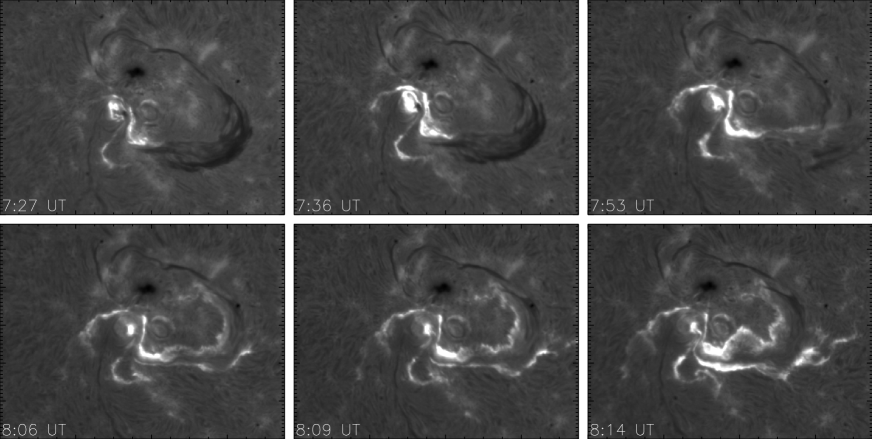
Figure 1: The M3.9, 2N flare observed in H_α at Udaipur Solar Observatory on November 18, 2003 in NOAA AR 10501.

Observations from GOES X-ray satellite showed an M3.9 class flare starting in the active region NOAA AR 10501 at 8:00 UT and attaining peak intensity at 8:30 UT. Figure 1 shows the time-lapse H_α images of the flare which started at a location close to the southern sunspots, and spread along the neutral line assuming the shape of a classic two-ribbon flare. The southern portion of the circular filament was blown off at 7:53 UT, which coincides with the timing of the launch of the associated CME. As a matter of fact, two CMEs were recorded in this active region on 18 November, at 8:06 UT and 08:50 UT. The first CME was associated with an M3.2 flare and was confined mostly to the southeast with minimal overlap with the earth direction, therefore the magnetic cloud of November 20 was identified to be associated with the the second CME. This eventually led to the strongest geomagnetic storm at the earth (Gopalswamy 2005b and Srivastava 2005a). In fact there were other CMEs on November 19 from the same region but they were too slow to be considered as the source of the observed magnetic cloud.

3 Data Analysis and Discussion

We analysed a series of magnetograms taken at 1 minute cadence during November $17-19$, 2003. For the analysis, we selected 168 images spanning the above period with an interval of 15 minutes. The bad images in the data-set were replaced by the ones closest in time. The images were first corrected for the solar rotation taking the last image on 18 November as the reference and then registered using a two-dimensional cross-correlation program. From these full disk magnetograms, a smaller region covering the AR 10501 including the filament channel was extracted for analysis.

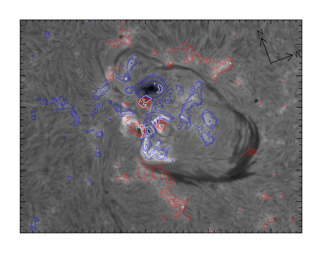
Figure 2: The magnetic field contours obtained from the line-of-sight MDI magnetogram, overlaid on H_α image obtained from the Udaipur Solar Observatory. Both the images were recorded at 6:24 UT. The red and blue contours here denote the positive and negative polarities respectively with field strength values of 1500, 1000, 200 and 100 G. The white contours overplotted on this image are the locations of strong magnetic field gradient derived from the line-of-sight magnetogram recorded at the same time. The two boxes correspond to the sub-areas considered for the study of magnetic flux evolution in MDI magnetograms shown in Figure 3.

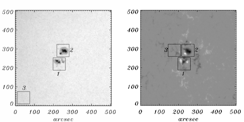
Figure 3: The left and right panels show the MDI continuum image and magnetogram taken on 18 November, respectively for the active region NOAA 10501. We studied the evolution of magnetic flux, average gradients in this region at 3 different locations marked by square boxes and named as 1,2,3. In order to compare, we chose these three regions to include northern sunspot of the AR in Box 2, southern sunspot in Box ‘1’ and relatively quiet region in Box 3. These three regions were $67\times 67$ arc-sec² size with the box size of $34\times 34$ pixels with each pixel corresponding to 1.98 arc-sec.

Figure 2 shows an overlay of the magnetic field contours obtained from one of the magnetograms taken at 06:24 UT on an H_α image taken around the same time. The H_α image and the magnetogram were co-aligned to contain the same area of interest. These co-aligned images were used to identify some of the sub-areas within the active region where most of the changes in magnetic flux or the initial flare activity in H_α images were observed. The sub-areas were chosen as a box of 1 arc-min size to accomodate the sunspot as well as its neighbouring region to detect any anomalous changes in the above mentioned quantities that might have led to flare. Considering the size of the sunspots, an optimum size of the box was chosen to include its neighbouring region as well. Choosing a larger box size would make it difficult to ascertain which region was responsible for the changes in the aforementioned parameters and a small box size would lead to a contamination by both emergence of flux as well motion of magnetic inhomogeneities, a consequence of the poor resolution of the magnetograms. The sub-regions are marked with boxes in Figure 3. The fact that there is no correlation in the flux in the two selected boxes 1 and 2 (cf. Figure 4) implies that variation of flux is consistent for the size of the box although a threshold value was not set as stated by Lara et al. (2000). It may be noted here that the source active region contains sunspots which are extremely complex as both the main spots have umbrae of opposite polarities within the same penumbra. Further, the initiation of the flare took place close to the umbrae of the sunspots in the box, labeled as ’1’. Using the magnetograms, a number of parameters were estimated for this active region such as magnetic potential energy, magnetic flux and magnetic field gradient.

The magnetic energy for a potential field configuration was computed for the active region using the virial theorem (Wheatland and Metcalf, 2006; Metcalf et al. 2008)

$$E_{p}=\frac{1}{4\pi}\int(xB_{px}+yB_{py})B_{z}dxdy$$ (1)

where E_p is the available potential energy in the region of interest. The origin of the coordinate system here is taken to be the center of the region of interest. The photospheric magnetic field components, B_px and B_py in x and y directions have been computed under the assumption of a potential magnetic field using Fast Fourier Transform (FFT) described by Alissandrakis (1981). These potential field components were then used to compute the magnetic energy using Equation 1. The parameters x and y signify the distance on the Sun having a transverse field B_x and B_y respectively.

Further, we estimated the magnetic flux in the active region using

$$\int{B_{z}da}$$ (2)

for the positive and negative polarities of the active region separately, where da is the elemental area. The magnetic field gradient in the active region can be computed using the following equation:

$$\nabla B_{z}=\sqrt{\left(\frac{dB_{z}}{dx}\right)^{2}+\left(\frac{dB_{z}}{dy}\right)^{2}}$$ (3)

3.1 Magnetic flux variation in the AR 10501

The SoHO/MDI magnetograms measure the line–of–sight component of the magnetic field, B_z. The area within which the flux is calculated is the selected area of the active region in each pixel. This was determined using the image scale and the angular scale of the Sun from the image header, which corresponds to $1409\times 1409$ km². The magnetic flux of positive and negative polarity was computed separately for each sub-region marked by boxes in Figure 3. Then, the variation of magnetic flux with time was studied (Figure 4). The figure shows that the negative flux for both the regions ’1’ and ’2’ and the positive flux in the region ’1’ show an increase with time, until 8:30 UT on November 18. This time coincides with the time of the M3.9 flare/halo CME on this day. After 8:30 UT, the magnetic flux values decreased.

In the region 1, the negative flux increased from 2.5 to 3.0 $\times 10^{21}$ Mx and then decreased to a value of 1.62$\times 10^{21}$ Mx after the flare/CME on November 18. The positive flux increased from $1.3\times 10^{21}$ Mx to $1.8\times 10^{21}$ Mx. On the other hand, region 2 showed an increase in the negative flux from 4.8 $\times 10^{21}$ Mx to 5.5 $\times 10^{21}$ Mx. This region shows negligible variation in the positive flux. The positive and negative flux in the region 3 show no variation, as expected, since the noise in the magnetogram is of the order of $\pm 10$ G (Scherrer et al. 1995).

Although the magnitude of the negative flux is higher (almost twice) in region 2 than in region 1 the rate of the increase of negative flux in both the regions is approximately the same, ($\sim 5.5\times 10^{15}$ Mx s^-1). It is found that in region 1, the positive flux also increased slowly with time, with absolute values higher than those of region 2. Thus, in region 1, the total flux increase is due to the increase in both the fluxes; while in region 2, the total flux increase is entirely due to the increase in the negative polarity flux. An overall increase in the absolute flux until the time of flare indicates that the emergence of new flux in the active region might have played a key role in triggering this flare/CME, particularly, in region 1. These indicate that the initiation of the flare is well correlated with the evolution of flux.

3.2 Variation of magnetic field gradient

We also estimated the value of average magnetic field gradient for the three small regions marked in Figure 5. Our measurements showed that the average gradient peaked to $\sim 90$ G Mm^-1 just before the flare in region 1. Region 2 also shows a sharp rise in the average gradient to 84 G Mm ^-1 before the flare. While there is a conspicuous rise in the average field gradient in both the regions, there are minor peaks in between that are possibly related to several other minor flares/CMEs which were launched from the same active region. An overlay of the gradient of magnetic field shows that the maximum gradient $\sim 90$ G Mm^-1 and occurred at the location where the flare kernel first appeared in H_α. It is to be noted that the flux and gradient seem to be well correlated. The plots also indicates that the initiation of the flare is well correlated with the magnetic field gradient in the region it occurred.

3.3 Variation in the magnetic energy

The magnetic potential energy calculated for the three small regions marked as 1, 2 and 3 show that the magnetic energy is the highest for the region 2 and of the order of $10^{32}$ ergs (Figure 6). For the regions 1 and 3, the magnetic energy is smaller of the order of $10^{31}$ and $10^{30}$ ergs respectively. One of the explanation for the large values of the magnetic energy in region 2 is that it includes a full big sunspot, which entails high magnetic flux and hence higher magnetic energy.

We measured the magnetic energy of the entire NOAA AR10501 for comparison, using the code developed by Wiegelmann (2004) to extrapolate the coronal magnetic field lines with vector magnetograms as input. These magnetograms were pre-processed with the help of a minimization method as described in Wiegelmann et al (2006). This method is superior to both the potential field extrapolation model and the linear force-free field extrapolation models as shown by Wiegelmann et al. (2005). The former has been used by several authors to compute the potential energy, because of its simplicity, (Forbes 2000, Venkatakrishnan and Ravindra, 2003, Gopalswamy et al. 2005a). However, it has been found that both these models are too simplistic to estimate the magnetic energy and the magnetic topology accurately (Schrijver et al. 2006 and Wiegelmann, 2008 and references therein). We compared the potential field energy of the entire active region NOAA 10501 on 17 (01:44 UT) and 18 November 2003 (00:20 UT) using the vector magnetogram data obtained from the Solar Flare Telescope at Mitaka. The entire computational box of 256x240x200 pixels size was chosen. Here, 1 pixel has a size of 1.32 arc-sec. The extrapolated field lines have been plotted in Figure 7. It is obvious from the plot that the field lines are highly twisted and non-potential close to region 1, and over the neighbouring curved filament in the active region which eventually erupted. The calculation shows that the magnetic energy over the entire active region is of the same order as that of region 2. The errors in the magnetic energy calculation using Wiegelmann (2004) code has been estimated to be within 3-4% for cases where the majority of magnetic flux is located sufficiently far away from the lateral boundaries of computational box and about 34% if high magnetic flux occur close to the boundaries (Schrijver et al. 2006; Wiegelmann et al. 2006, 2008). For the active region for which the magnetic energy has been calculated in this paper, the majority of the flux is located far from lateral boundaries of the computational box and magnetic strength flux is low close to the side boundaries. Therefore, one can consider an error of less than 5% in the estimated magnetic energy.

Table 1: Estimates of the energy for the NOAA AR10501

Date	Potential field	NLFF	Max Free
Time	Energy (ergs)	Energy (ergs)	Energy (ergs)
17 Nov 2003	$4.07(\pm 0.20)\times 10^{32}$	$6.72(\pm 0.34)\times 10^{32}$	$2.65(\pm 0.13)\times 10^{32}$
01:44 UT
18 Nov 2003	$3.3(\pm 0.17)\times 10^{32}$	$5.65(\pm 0.28)\times 10^{32}$	$2.35(\pm 0.12)\times 10^{32}$
00:20 UT

From Table 1, it is evident that the magnetic potential energy arising from a nonlinear force free field in the Active Region NOAA 10501 was higher on November 17, 2003 than on November 18, 2003, even before the CME took off. This can be reasonably explained by the fact that the same active region triggered off another CME the previous day i.e. 17 November at 8:57 UT. This CME was observed as a partial halo CME recorded by LASCO coronagraphs and was associated with an M4.2, 1N class flare. However, because of lack of co-temporal vector magnetograms, it is difficult to confirm this explanation.

Further, it is well established that it is the magnetic free energy in an active region that powers an ensuing coronal mass ejection and that the maximum speed of the coronal mass ejection is constrained by the maximum free energy available in the source region. As pointed out by Metcalf et al. (1995), free energy in the magnetic fields can be estimated from the distribution of the current in the coronal layers. Table 1 also shows that the maximum free energy available on November 17 and 18 is respectively, about $0.65(\pm 0.0325)$ and $0.7(\pm 0.035)$ times that of the corresponding estimated potential energy. Here, the errors in the computed magnetic energy has been estimated to be less than $5\%$ (Schrijver et al. 2006, Wiegelmann et al. 2008). This suggests that the assumption that the available potential energy may be a good indicator of the free energy may not always be true, as has been assumed by several authors viz. Venkatakrishnan and Ravindra (2003), Gopalswamy et al. (2005a) in the absence of vector magnetograms. For better estimates of the available free energy, vector magnetograms taken at a higher cadence are required.

3.4 Magnetic energy and CME speeds

The maximum projected plane-of-sky speed of the CMEs of November 17 and 18 (as estimated from the LASCO/SoHO coronagraph data) were of the order of 1000 km s^-1 and 1660 km s^-1, respectively. It is important to mention here that the flare classification in X-ray for the November 17 flare is M4.2, which is relatively higher than the M3.9 for the November 18 flare. Further, the free energy available on November 17 is higher compared to that on November 18, but the CME speed is higher for the latter.

We obtained the mass of the CMEs of November 17 and 18, 2003 (Vourlidas 2009, Private Communication). We then computed the kinetic energy of the CMEs under study using the measured values of the speeds of the CMEs. The estimated maximum kinetic energy for the CME of November 17 is about $0.3\times 10^{32}$ ergs. It may be pointed out here that the kinetic energy estimate can be uncertain by a factor of 2 because of the uncertainty involved in estimation of the CME mass (Vourlidas et al. 2000). However, even with this uncertainty, kinetic energy is only a fraction of the maximum free energy, suggesting that only a fraction of the maximum free energy was spent in launching the CME. On the other hand, we found that the estimated kinetic energy of the CME on the November 18 is $3.3\times 10^{32}$ ergs, a value higher than the available free energy. the reason for this discrepancy, may be well due to the uncertainties involved in measurement of the kinetic energy.

As mentioned above, due to uncertainty in the measurement of mass, the measured kinetic energy is uncertain by a factor of 2. Taking this into account we find that the kinetic energy of the CME on November 17, CME can vary from $1.6\times 10^{31}$ to $6.4\times 10^{31}$ ergs, which approximately corresponds to 5.5% and 22% of the available free energy. Although the observations are not co-temporal as in the case of November 18 CME, the estimated kinetic energy with the given uncertainty is still less than the estimated free energy.

If we extend the same argument to the CME of November 18, it is observed that the uncertainty in the estimated kinetic energy varies from $1.65\times 10^{32}$ to $6.6\times 10^{32}$ ergs. If one assumes the former value, the kinetic energy is approximately 70% of the available free energy while the latter exceeds the available free energy by a factor of 2.8. Since we are limited by lack of simultaneous observations, it would be inappropriate to quantify the small yet finite difference in available free energy in the active region and the estimated kinetic energy of the CME on November 18 CME originating from same active region.

Another possibility for this discrepancy could be the fact that the free energy on November 18 was calculated for the time at which the vector magnetogram was available, which was eight hours before the CME was actually launched. There is a possibility that the free energy was lower at this instant and had since risen. This is supported by the argument that the plot of the magnetic potential energy derived from the line-of-sight MDI magnetograms shows a rise during this phase. It is more likely that the total energy is also large owing to increase in magnetic flux. This also underscores the importance of obtaining regular vector magnetograms at a higher cadence. A study of source regions of geo-effective CMEs in this cycle using Hinode vector magnetograph observations may be extremely helpful to resolve similar issues.

4 Summary and Conclusion

The analysis of the magnetic field data of the source active region of November 18, 2003 CME, before, during and after the flare, lead to the following inferences.

Of the three regions, region 2 possesses the largest magnetic energy, and magnetic flux. It also shows a steeper rise in the magnetic field gradient than the other two regions. This indicates that initiation of the flare may occur at this region. However, the flare in H_α initiated at a location that is marked by high average gradient and the emergence of fluxes of both polarities. In fact, the rate of increase of magnetic flux is the same for both the regions 1 and 2. Moreover, the region associated with the flare/CME onset is also marked by twisted non-potential low-lying field lines, while region 2 is marked by straight non-twisted open field lines, as evident from the field line extrapolation. It is to be kept in mind that here the definition of open field lines here signify the field lines which pass through the upper boundary (200 pixel or 264 arc-sec). These ’open field lines’ do not close within the active region. It is not possible to distinguish, if they are globally open or connected to areas outside the considered active region.

This indicates that the best configuration for reconnection may have occurred in region 1, because new fluxes of both polarities emerge and maintain a high magnetic gradient in the small region chosen for the analysis. Once the flare is initiated and spreads in the shape of two-ribbons the field lines then get reconnected to the twisted magnetic field lines over the filament, leading to its destabilization and eruption as a whole. The extrapolation of non-linear 3-D force free field lines above the active region is shown in Figure 7. This clearly shows the twisted field lines above the filament which erupted with the flare and associated CME.

1. The pre-flare configuration of the active region NOAA AR 10501 is marked by emergence of flux in both polarities thereby increasing the total flux and high magnetic gradient of the order of 90 Mx s^-1 at a localized site of flare initiation.

2. The time of the initiation of the flare is well correlated with the evolution of the flux and gradient in the region it first appeared.

3. The nonlinear force-free field line extrapolation shows that the region of the flare/CME onset is marked by twisted non-potential low-lying field lines as compared to the other region, which is marked by straight open field lines as evident from the field line extrapolation. The flare triggered the reconnection of the field lines overlying the neighbouring filament in the active region which is also highly non-potential in nature.

4. The total magnetic potential energy of the active region was estimated to be of the order of 10³² ergs. The magnetic energy of the active region increased continuously before the flare.

5. The maximum free energy available in the active region is approximately 0.7 times that of the potential energy.

Figure 4: This figure shows evolution of the positive and negative magnetic flux in the separate boxes marked by 1,2,3 in Figure 3. The positive and negative flux for the three regions are shown as asterix, diamond, square box, triangle, open circles and filled circles respectively. The x-axis indicates time with start time as 0 UT on 17 November. The vertical line at 32.5 hour coincides with the peak of the flare. The discontinuity in the plots indicates a gap in the data recorded by the MDI instrument.

Figure 5: Evolution of magnetic field gradient for the regions 1 and 2 in Gauss per Mm. The plots show an increase in the magnetic field gradient for both the regions.

Figure 6: This plot shows the evolution of the magnetic potential energy (measured in ergs) with time, in the separate regions marked by 1,2.

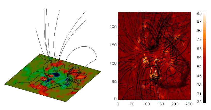
Figure 7: The above figure shows the nonlinear extrapolated magnetic field lines in the NOAA AR10501 from the vector magnetogram data obtained on 18 November at 00:20 UT from the Solar flare telescope at Mitaka. For this purpose, we considered the entire box of $256\times 240\times 240$ pixels, where 1 pixel =1.32 arc-sec and used the technique for field extrapolation developed by Wiegelmann (2004). The non-linear force free extrapolation field lines (shown in black) have been overplotted in this figure. The size of the magnetogram is $256\times 240$ pixels in x and y directions respectively. The field has been extrapolated to 200 pixels in the z-direction. On the right is shown the projection of both open and closed field lines onto the H_α image

.