Semiclassical analysis of Schrödinger operators with magnetic wells

Abstract.

We give a survey of some results, mainly obtained by the authors and their collaborators, on spectral properties of the magnetic Schrödinger operators in the semiclassical limit. We focus our discussion on asymptotic behavior of the individual eigenvalues for operators on closed manifolds and existence of gaps in intervals close to the bottom of the spectrum of periodic operators.

1. Preliminaries

1.1. The magnetic Schrödinger operators

Let $(M,g)$ be an oriented Riemannian manifold of dimension $n\geq 2$. Let $\bf B$ be a real-valued closed $C^{\infty}$ 2-form on $M$. Assume that $\bf B$ is exact and choose a real-valued $C^{\infty}$ 1-form $\bf A$ on $M$ such that $d{\bf A}=\bf B$.

Thus, one has a natural mapping

$$u\mapsto i\,du+{\bf A}u$$

from $C^{\infty}_{c}(M)$ to the space $\Omega^{1}_{c}(M)$ of smooth, compactly supported one-forms on $M$. The Riemannian metric allows to define scalar products in these spaces and consider the adjoint operator

$$(i\,d+{\bf A})^{*}:\Omega^{1}_{c}(M)\to C^{\infty}_{c}(M).$$

A Schrödinger operator with magnetic potential $\bf A$ is defined by the formula

$$H_{\bf A}=(i\,d+{\bf A})^{*}(i\,d+{\bf A}).$$

From the geometric point of view, we may regard $\bf A$ as a connection one form of a Hermitian connection on the trivial line bundle $\mathcal{L}$ over $M$, defining the covariant derivative $\nabla_{\bf A}=d-i{\bf A}$. The curvature of this connection is $-i\bf B$. Then the operator $H_{\bf A}$ coincides with the covariant (or Bochner) Laplacian:

$$H_{\bf A}=\nabla_{\bf A}^{*}\nabla_{\bf A}.$$

Choose local coordinates $X=(X_{1},\ldots,X_{n})$ on $M$. Write the 1-form $\bf A$ in the local coordinates as

$${\bf A}=\sum_{j=1}^{n}A_{j}(X)\,dX_{j},$$

the matrix of the Riemannian metric $g$ as

$$g(X)=(g_{j\ell}(X))_{1\leq j,\ell\leq n}$$

and its inverse as

$$g(X)^{-1}=(g^{j\ell}(X))_{1\leq j,\ell\leq n}.$$

Denote $|g(X)|=\det(g(X))$. Then the magnetic field $\bf B$ is given by the following formula

$${\bf B}=\sum_{j<k}B_{jk}\,dX_{j}\wedge dX_{k},\quad B_{jk}=\frac{\partial A_{k}}{\partial X_{j}}-\frac{\partial A_{j}}{\partial X_{k}}.$$

Moreover, the operator $H_{\bf A}$ has the form

$$H_{\bf A}=\frac{1}{\sqrt{|g(X)|}}\sum_{1\leq j,\ell\leq n}\left(i\frac{\partial}{\partial X_{j}}+A_{j}(X)\right)\left[\sqrt{|g(X)|}g^{j\ell}(X)\left(i\frac{\partial}{\partial X_{\ell}}+A_{\ell}(X)\right)\right].$$

When $n=2$, the magnetic two-form $\bf B$ is a volume form on $M$ and therefore can be identified with the function $b\in C^{\infty}(M)$ given by

$${\bf B}=b\,dx_{g},$$

where $dx_{g}$ denotes the Riemannian volume form $M$ associated with $g$.

When $n=3$, the magnetic two-form $\bf B$ can be identified with a magnetic vector field $\vec{b}$ by the Hodge star-operator. If $M$ is the Euclidean space ${\mathbb{R}}^{3}$, we have

$$\vec{b}=(b_{1},b_{2},b_{3})=\operatorname{curl}{\bf A}=(B_{23},-B_{13},B_{12})$$

with the usual definition of $\operatorname{curl}$.

We will consider the magnetic Schrödinger operator $H_{\bf A}$ as an unbounded operator in the Hilbert space $L^{2}(M)$. We will discuss two cases:

• $M$ is a compact manifold, possibly with boundary;

• $M$ is a noncompact oriented manifold equipped with a properly discontinuous action of a finitely generated, discrete group $\Gamma$ such that $M/\Gamma$ is compact.

In the first case, if $M$ has non-empty boundary, we will assume that the operator $H^{h}$ satisfies the Dirichlet boundary conditions. Moreover, we will only consider the case when the potential wells defined by the magnetic field lie in the interior of $M$. A closely related case is the case $M=\mathbb{R}^{2}$ under the assumption that the potential wells defined by the magnetic field lie in a compact subset of $\mathbb{R}^{2}$ and that $\liminf_{|x|\rightarrow+\infty}b(x)>\inf b$.

In the second case, we will assume that $M$ is complete and $H^{1}(M,{\mathbb{R}})=0$, i.e. any closed $1$-form on $M$ is exact. Moreover, the metric $g$ and the magnetic 2-form $\bf B$ are supposed to be $\Gamma$-invariant (but $\bf A$, in general, is not $\Gamma$-invariant). Moreover, we will assume that the magnetic field has a periodic set of compact potential wells (see Section 4 for a precise definition).

In both cases, if $M$ is without boundary (this is always true in the second case), the operator $H_{\bf A}$ is essentially self-adjoint with domain $C^{\infty}_{c}(M)$. In the case when $M$ has non-empty boundary, we will consider the self-adjoint operator obtained as the Friedrichs extension of the operator $H_{\bf A}$ with domain $C^{\infty}_{c}(M)$ (the Dirichlet realization). We refer the reader to the book [5] (and the references therein), for the description of the spectral properties of the Neumann realization of a magnetic Schrödinger operator on a compact manifold with boundary and their applications to problems in superconductivity and liquid crystals. We also refer the reader to the surveys [3, 7, 8, 25] for the presentation of general results concerning the Schrödinger operator with magnetic fields.

We will discuss spectral properties of the magnetic Schrödinger operator in the semiclassical limit. So we consider the operator $H^{h}$, depending on a semiclassical parameter $h>0$, defined as

$$H^{h}=(ih\,d+{\bf A})^{*}(ih\,d+{\bf A}).$$

The operators $H^{h}$ and $H_{\bf A}$ are related by the formula

$$H^{h}=h^{2}(\,d-ih^{-1}{\bf A})^{*}(\,d-ih^{-1}{\bf A})=h^{2}H_{h^{-1}\bf A}.$$

This formula shows, in particular, that the semiclassical limit $h\to 0$ is clearly equivalent to the large magnetic field limit.

1.2. Magnetic wells

For any $x\in M$, denote by $B(x)$ the linear operator on the tangent space $T_{x}{M}$ associated with the 2-form $\bf B$:

$$g_{x}(B(x)u,v)={\bf B}_{x}(u,v),\quad u,v\in T_{x}{M}.$$

In local coordinates $X=(X_{1},\ldots,X_{n})$, the matrix $(b^{\alpha}_{\beta}(X))_{\alpha,\beta=1,\ldots,n}$ of $B(X)$ is given by

$$b^{\alpha}_{\beta}(X)=\sum_{j=1}^{n}B_{\beta j}(X)g^{j\alpha}(X).$$

It is easy to check that $B$ is skew-adjoint with respect to $g$, and therefore for each $x\in M$ the non-zero eigenvalues of $B(x)$ can be written as $\pm i\lambda_{j}(x)$, where $\lambda_{j}(x)>0$, $j=1,2,\ldots,d$. Introduce the function (the intensity of the magnetic field)

$${\mbox{\rm Tr}}^{+}(B(x))=\sum_{j=1}^{d}\lambda_{j}(x)=\frac{1}{2}\mbox{\rm Tr}([B^{*}(x)\cdot B(x)]^{1/2}).$$

We will also use the trace norm of $B(x)$:

$$|B(x)|=[\mbox{\rm Tr}(B^{*}(x)\cdot B(x))]^{1/2}\,.$$

It coincides with the norm of $B(x)$ with respect to the Riemannian metric on the space of tensors of type $(1,1)$ on $T_{x}M$ induced by the Riemannian metric $g$ on $M$. In local coordinates $X=(X_{1},\ldots,X_{n})$, we have

$$|B(X)|=\left(\sum_{i,j,k,\ell}g^{ij}(X)g_{k\ell}(X)b_{i}^{k}(X)b_{j}^{\ell}(X)\right)^{1/2}\,.$$

When $n=2$, then

$${\mbox{\rm Tr}}^{+}(B(x))=|b(x)|\ \text{and}\ |B(x)|=\sqrt{2}\,|b(x)|\,.$$

When $n=3$, then

$${\mbox{\rm Tr}}^{+}(B(x))=|\vec{b}(x)|\ \text{and}\ |B(x)|=\sqrt{2}\,|\vec{b}(x)|\,.$$

Remark that the function $|B(x)|^{2}$ is clearly $C^{\infty}$, whereas the function ${\mbox{\rm Tr}}^{+}B$ is only continuous (more precisely, it is locally Hölder of order $1/2n$ (see [18] and references therein)). It turns out that in many spectral problems the function $x\mapsto h\cdot{\mbox{\rm Tr}}^{+}(B(x))$ can be considered as a magnetic potential, that is, as a magnetic analog of the electric potential $V$ in a Schrödinger operator $-h^{2}\Delta+V$. This leads us to introduce the notion of magnetic well as follows.

Let $b_{0}$ be the minimal intensity of the magnetic field

$$b_{0}=\min\{{\mbox{\rm Tr}}^{+}(B(x))\,:\,x\in{M}\}.$$

Consider the zero set of ${\mbox{\rm Tr}}^{+}(B(x))-b_{0}$

$$U=\{x\in M:{\mbox{\rm Tr}}^{+}(B(x))=b_{0}\}\,.$$

A magnetic well (attached to the given energy $hb_{0}$) is by definition a connected component of $U$. If $M$ is compact and has non-empty boundary, we will always assume that $U$ is included in the interior of $M$.

1.3. Rough estimates for the lowest eigenvalue

Assume that $M$ is a compact manifold. Denote by $\lambda_{0}(H^{h})$ the bottom of the spectrum of the operator $H^{h}$ in $L^{2}(M)$.

Theorem 1.1 ([14], Theorem 2.2).

For any $\mu\in\operatorname{Im}{\mbox{\rm Tr}}^{+}B$, there exists $C>0$ and $h_{0}>0$ such that, for any $h\in(0,h_{0}]$ ,

$$(-C\,h^{4/3}+h\mu,h\mu+C\,h^{4/3})\neq\emptyset\,.$$

Moreover, there exists $C>0$ such that

$$-C\,h^{5/4}\leq\lambda_{0}(H^{h})-hb_{0}\leq C\,h^{4/3}.$$

The last result can be improved if the rank of ${\bf B}$ is constant. This can be seen as a form of the Melin-Hörmander inequality. Using the techniques developed in [18] one can indeed get the existence of $C>0$ and $h_{0}>0$ such that, for any $h\in(0,h_{0}]$ ,

$$-C\,h^{2}\leq\lambda_{0}(H^{h})-hb_{0}\,.$$

Remark that if $n=2$ and $M$ is without boundary then we necessarily have $b_{0}=0$, since

$$\int_{M}b(x)dx_{g}=\int_{M}d{\bf A}=0\,.$$

If we suppose that $M$ has non-empty boundary, the operator $H^{h}$ satisfies the Dirichlet boundary conditions and $b_{0}>0$, it was observed by many authors [26, 24, 30] (as the immediate consequence of the Weitzenböck-Bochner type identity and the positivity of the square of a suitable Dirac operator) that

$$\inf\sigma(H_{\bf A})\geq b_{0}\,,$$

where $\sigma(H_{\bf A})$ denotes the spectrum of the operator $H_{\bf A}$ in $L^{2}(M)$ and, as a consequence, that, for any $h>0\,$,

$$\lambda_{0}(H^{h})\geq hb_{0}\,.$$

In the case $M=\mathbb{R}^{2}$, this estimate follows from the formula

$$b(x)=-i[D_{x_{1}}-A_{1},D_{x_{2}}-A_{2}]\,,$$

where, as usual, $D_{x_{k}}=\frac{1}{i}\frac{\partial}{\partial x_{k}}$, $k=1,2$, which implies (after an integration by parts) that

$$\int b(x)|u(x)|^{2}\,dx\leq\|(D_{x_{1}}-A_{1})u\|^{2}+\|(D_{x_{2}}-A_{2})u\|^{2}\;.$$

If $b_{0}=0$, one prove a more precise estimate for $\lambda_{0}(H^{h})$ in the case when the magnetic wells are regular submanifolds. Denote by $d(x,y)$ the geodesic distance between $x$ and $y$.

Theorem 1.2 ([14], Theorem 2.4).

Let us assume that $b_{0}=0$ and that $U$ is a $C^{\infty}$ compact submanifold of $M$ included in the interior in $M$. If there exist $k\in{\mathbb{Z}}_{+}$, $C_{1}$ and $C_{2}>0$ such that if $d(x,U)<C_{2}$

$$C_{1}^{-1}\,d(x,U)^{k}\leq|B(x)|\leq C_{1}\,d(x,U)^{k}\,,$$

then one can find $h_{0}$ and $C>0$ such that, for any $h\in(0,h_{0}]\,$,

$$C^{-1}\,h^{(2k+2)/(k+2)}\leq\lambda_{0}(H^{h})\leq C\,h^{(2k+2)/(k+2)}\,.$$

2. Discrete wells

In this section, we continue to assume that $M$ is compact. Denoting by $\lambda_{0}(H^{h})\leq\lambda_{1}(H^{h})\leq\lambda_{2}(H^{h})\leq\ldots$ the eigenvalues of the operator $H^{h}$ in $L^{2}(M)$, we will consider the case when the magnetic wells are points.

2.1. The case $b_{0}=0$

Let us assume that $b_{0}=0$, and, for some integer $k>0$, if $B(x_{0})=0$, then $x_{0}$ belongs to the interior of $M$ and there exists a positive constant $C$ such that for all $x$ in some neighborhood of $x_{0}$ the estimate holds:

$$C^{-1}\,d(x,x_{0})^{k}\leq{\mbox{\rm Tr}}^{+}(B(x))\leq C\,d(x,x_{0})^{k}.$$

In this case, the important role is played by a differential operator $K^{h}_{\bar{x}_{0}}$ in ${\mathbb{R}}^{n}\,$, which is in some sense an approximation to the operator $H^{h}$ near $x_{0}\,$. Recall its definition [14].

Let $\bar{x}_{0}$ be a zero of $B$. Choose local coordinates $f:U(\bar{x}_{0})\to{\mathbb{R}}^{n}$ on $M$, defined in a sufficiently small neighborhood $U(\bar{x}_{0})$ of $\bar{x}_{0}$. Suppose that $f(\bar{x}_{0})=0$, and the image $f(U(\bar{x}_{0}))$ is a ball $B(0,r)$ in ${\mathbb{R}}^{n}$ centered at the origin.

Write the $2$-form $\bf B$ in the local coordinates as

$${\bf B}(X)=\sum_{1\leq l<m\leq n}b_{lm}(X)\,dX_{l}\wedge dX_{m}\,,\quad X=(X_{1},\ldots,X_{n})\in B(0,r).$$

Let ${\bf B}^{0}$ be the closed 2-form in ${\mathbb{R}}^{n}$ with polynomial components defined by the formula

$${\bf B}^{0}(X)=\sum_{1\leq l<m\leq n}\sum_{|\alpha|=k}\frac{X^{\alpha}}{\alpha!}\frac{\partial^{\alpha}b_{lm}}{\partial X^{\alpha}}(0)\,dX_{l}\wedge dX_{m}\,,\quad X\in{\mathbb{R}}^{n}.$$

One can find a 1-form ${\bf A}^{0}$ on ${\mathbb{R}}^{n}$ with polynomial components such that

$$d{\bf A}^{0}(X)={\bf B}^{0}(X)\,,\quad X\in{\mathbb{R}}^{n}.$$

Let $K^{h}_{\bar{x}_{0}}$ be a self-adjoint differential operator in $L^{2}({\mathbb{R}}^{n})$ with polynomial coefficients given by the formula

$$K_{\bar{x}_{0}}^{h}=(ih\,d+{\bf A}^{0})^{*}(ih\,d+{\bf A}^{0})\,,$$

where the adjoints are taken with respect to the Hilbert structure in $L^{2}({\mathbb{R}}^{n})$ given by the flat Riemannian metric $(g_{lm}(0))$ in ${\mathbb{R}}^{n}$. If ${\bf A}^{0}$ is written as

$${\bf A}^{0}=A^{0}_{1}\,dX_{1}+\ldots+A^{0}_{n}\,dX_{n}\,,$$

then $K^{h}_{\bar{x}_{0}}$ is given by the formula

$$K_{\bar{x}_{0}}^{h}=\sum_{1\leq l,m\leq n}g^{lm}(0)\left(ih\frac{\partial}{\partial X_{l}}+A^{0}_{l}(X)\right)\left(ih\frac{\partial}{\partial X_{m}}+A^{0}_{m}(X)\right).$$

The operators $K^{h}_{\bar{x}_{0}}$ have discrete spectrum (cf, for instance, [17, 15]). Using the simple dilation $X\mapsto h^{\frac{1}{k+2}}X$, one can show that the operator $K^{h}_{\bar{x}_{0}}$ is unitarily equivalent to $h^{\frac{2k+2}{k+2}}K^{1}_{\bar{x}_{0}}\,$. Thus, $h^{-\frac{2k+2}{k+2}}K^{h}_{\bar{x}_{0}}$ has discrete spectrum, independent of $h$.

Under the current assumptions, the zero set $U$ of ${\bf B}$ is a finite collection of points:

$$U=\{\bar{x}_{1},\ldots,\bar{x}_{N}\}\,.$$

Let $K^{h}$ be the self-adjoint operator on $L^{2}(T_{\bar{x}_{1}}M)\oplus\cdots\oplus L^{2}(T_{\bar{x}_{N}}M)$ defined by

(2.1) $$K^{h}=K^{h}_{\bar{x}_{1}}\oplus\cdots\oplus K^{h}_{\bar{x}_{N}}\,.$$

Let $\mu_{0}\leq\mu_{1}\leq\ldots$ be the increasing sequence of eigenvalues associated with $K^{h}$ for $h=1$.

Theorem 2.1 ([14], Theorem 2.5).

For any natural $m$, the eigenvalue $\lambda_{m}(H^{h})$ has an asymptotic expansion, when $h\to 0$, of the form

$$\lambda_{m}(H^{h})=h^{(2k+2)/(k+2)}[\mu_{m}+O(h^{1/(k+2)})]\,.$$

Moreover ([14, Proposition 2.7]), if $\mu$ is a non degenerate eigenvalue of $K^{h}_{\bar{x}_{j}}$, for some $j$, then there exists an eigenvalue $\lambda(H^{h})$ of $H^{h}$ which has a complete asymptotic expansion of the form

$$\lambda(H^{h})\sim h^{(2k+2)/(k+2)}\sum_{j=0}^{+\infty}a_{j}h^{j/(k+2)}\,,$$

with $a_{0}=\mu$.

2.2. The case $b_{0}\neq 0$

In this subsection, we consider the case when $M$ is a two-dimensional compact manifold and $b_{0}\neq 0$. We assume that $M$ has non-empty boundary and the operator $H^{h}$ satisfies the Dirichlet boundary conditions. Moreover, we suppose that there is a unique minimum point $\bar{x}_{0}$, which belongs to the interior of $M$, such that $b(\bar{x}_{0})=b_{0}$ and which is non degenerate:

$${\rm Hess}\,b(\bar{x}_{0})>0.$$

We introduce in this case the notation

$$a=\operatorname{Tr}\left(\frac{1}{2}{\rm Hess}\,b(\bar{x}_{0})\right)^{1/2}.$$

Theorem 2.2 ([16] , Theorem 7.2).

There exist a constant $C>0$ and $h_{0}>0$, such that, for $h\in(0,h_{0}]\,$,

$$-C\,h^{19/8}\leq\lambda_{0}(H^{h})-hb_{0}-\frac{a^{2}}{2b_{0}}h^{2}\leq C\,h^{5/2}\,.$$

The proof is based on the analysis of the simpler model in ${\mathbb{R}}^{2}$ where near $0$

$$b(x,y)=b_{0}+\alpha x^{2}+\beta y^{2}\,.$$

In this case one can also choose a gauge ${\bf A}=A_{1}(x,y)dx+A_{2}(x,y)dy$ such that

$$A_{1}(x,y)=0\quad\text{and}\quad A_{2}(x,y)=b_{0}+\frac{\alpha}{3}x^{3}+\beta xy^{2}\,.$$

We mention two open problems in this setting:

1. Proof of the existence of a complete asymptotic expansion for $\lambda_{0}(H^{h})$ in the two-dimensional case.

2. Accurate analysis of the bottom of the spectrum in the three-dimensional case.

One should note that the situation is completely different when the Neumann boundary condition is considered. For a discussion of this case, we refer the reader to [4] and the references therein.

3. Hypersurface wells

In this section, we consider the case when $b_{0}=0$ and the zero set $U$ of the magnetic field is a smooth oriented hypersurface $S$. Moreover, there are constants $k\in{\mathbb{Z}}$, $k>0$, and $C>0$ such that, for all $x$ in a neighborhood of $S$, we have:

(3.1) $$C^{-1}\,d(x,S)^{k}\leq|B(x)|\leq C\,d(x,S)^{k}\,.$$

This model was introduced for the first time by Montgomery [26] and was further studied in [14, 27, 9, 12, 13].

We begin with a discussion of some family of ordinary differential operators, which play a very important role in the study of this case.

3.1. Some ordinary differential operators

For any $\alpha\in{\mathbb{R}}$ and $\beta\in{\mathbb{R}},\beta\neq 0$, consider the self-adjoint second order differential operator in $L^{2}({\mathbb{R}})$ given by

$$Q(\alpha,\beta)=-\frac{d^{2}}{dt^{2}}+\left(\frac{1}{k+1}\beta t^{k+1}-\alpha\right)^{2}.$$

In the context of magnetic bottles, this family of operators (for $k=1$) first appears in [26] (see also [14]). Denote by $\lambda_{0}(\alpha,\beta)$ the bottom of the spectrum of the operator $Q(\alpha,\beta)$.

Recall some properties of $\lambda_{0}(\alpha,\beta)$, which were established in [26, 14, 27]. First of all, $\lambda_{0}(\alpha,\beta)$ is a continuous function of $\alpha\in{\mathbb{R}}$ and $\beta\in{\mathbb{R}}\setminus\{0\}$. One can see by scaling that, for $\beta>0$,

(3.2) $$\lambda_{0}(\alpha,\beta)=\beta^{\frac{2}{k+2}}\,\lambda_{0}(\beta^{-\frac{1}{k+2}}\alpha,1)\,.$$

A further discussion depends on $k$ odd or $k$ even.

When $k$ is odd, $\lambda_{0}(\alpha,1)$ tends to $+\infty$ as $\alpha\rightarrow-\infty$ by monotonicity. For analyzing its behavior as $\alpha\rightarrow+\infty$, it is suitable to do a dilation $t=\alpha^{\frac{1}{k+1}}s$, which leads to the analysis of

$$\alpha^{2}\left(-h^{2}\frac{d^{2}}{ds^{2}}+\left(\frac{s^{k+1}}{k+1}-1\right)^{2}\right)\,,$$

with $h=\alpha^{-(k+2)/(k+1)}$ small. One can use the semi-classical analysis (see [2] for the one-dimensional case and [28, 19] for the multidimensional case) to show that

$$\lambda_{0}(\alpha,1)\sim(k+1)^{\frac{2k}{k+1}}\alpha^{\frac{k}{k+1}}\,,\;\mbox{ as }\alpha\rightarrow+\infty\,.$$

In particular, we see that $\lambda_{0}(\alpha,1)$ tends to $+\infty\,$.

When $k$ is even, we have $\lambda_{0}(\alpha,1)=\lambda_{0}(-\alpha,1)\,$, and, therefore, it is sufficient to consider the case $\alpha\geq 0\,$. As $\alpha\rightarrow+\infty$, semi-classical analysis again shows that $\lambda_{0}(\alpha,1)$ tends to $+\infty\,$.

So in both cases, it is clear that the continuous function $\lambda_{0}(\alpha,1)$ is positive:

$$\hat{\nu}:=\inf_{\alpha\in{\mathbb{R}}}\lambda_{0}(\alpha,1)\geq 0\,,$$

and there exists (at least one) $\alpha_{\mathrm{min}}\in{\mathbb{R}}$ such that $\lambda_{0}(\alpha,1)$ is minimal:

$$\lambda_{0}(\alpha_{\mathrm{min}},1)=\hat{\nu}\,.$$

The results of numerical computations for $\alpha_{\mathrm{min}}$, $\hat{\nu}$ and the second eigenvalue $\lambda_{1}$ of the operator $Q(\alpha_{\rm min},1)$ are given in Table 1.

$k$	1	2	3	4	5	6	7
$\alpha_{\mathrm{min}}$	0.35	0	0.16	0	0.10	0	0.07
$\hat{\nu}$	0.57	0.66	0.68	0.76	0.81	0.87	0.92
$\lambda_{1}$	1.98	2.50	2.61	2.98	3.18	3.47	3.66

Table 1. Numerical results for $\alpha_{\mathrm{min}}$, $\hat{\nu}$ and $\lambda_{1}$

In Figures 1 and 2, one can also see the graphs of the function $\lambda=\lambda_{0}(\alpha,1)$ and its quadratic approximation at $\alpha=\alpha_{\mathrm{min}}$:

$$\lambda^{\mathrm{quad}}(\alpha)=\lambda_{0}(\alpha_{\rm min},1)+\frac{1}{2}\frac{\partial^{2}\lambda_{0}}{\partial\alpha^{2}}(\alpha_{\mathrm{min}},1)(\alpha-\alpha_{\mathrm{min}})^{2}\,.$$

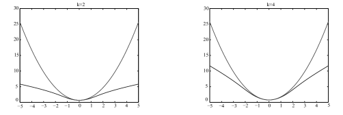
Figure 1. $k$ even

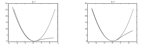
Figure 2. $k$ odd

Numerical computations show that when $k$ is even the minimum is attained at zero: $\alpha_{\rm min}=0\,$. They also suggest that the minimum $\alpha_{\rm min}$ is non degenerate:

$$\frac{\partial^{2}\lambda_{0}}{\partial\alpha^{2}}(\alpha_{\mathrm{min}},1)>0\,.$$

and that the second derivative $\frac{\partial^{2}\lambda_{0}}{\partial\alpha^{2}}(\alpha_{\mathrm{min}},1)$ tends as $k$ tends to $\infty$ to $2$.

Let $u^{0}_{\alpha}\in L^{2}({\mathbb{R}})$ be the $L^{2}$ normalized strictly positive eigenvector of the operator $Q(\alpha,1)$, corresponding to the eigenvalue $\lambda_{0}(\alpha,1)$:

$$Q(\alpha,1)u^{0}_{\alpha}=\lambda_{0}(\alpha,1)u^{0}_{\alpha},\quad\|u^{0}_{\alpha}\|=1\,.$$

One can show that $u^{0}_{\alpha}$ depends smoothly on $\alpha$. Then one can show that

$$\frac{\partial\lambda_{0}}{\partial\alpha}(\alpha,1)=-2\int\left(\frac{t^{k+1}}{k+1}-\alpha\right)(u^{0}_{\alpha}(t))^{2}\,dt$$

and

$$\frac{\partial^{2}\lambda_{0}}{\partial\alpha^{2}}(\alpha,1)=2-4\int\frac{t^{k+1}}{k+1}u^{0}_{\alpha}(t)\frac{\partial u^{0}_{\alpha}}{\partial\alpha}\,dt\,.$$

It follows that

$$\int\left(\frac{t^{k+1}}{k+1}-\alpha_{\mathrm{min}}\right)(u^{0}_{\alpha}(t))^{2}\,dt=0\,,$$

and, for $k$ odd, $\alpha_{\mathrm{min}}=\int\frac{t^{k+1}}{k+1}(u^{0}_{\alpha_{\mathrm{min}}}(t))^{2}\,dt>0\,$. It has been claimed that this minimum is unique for $k=1$ in [27] and for arbitrary odd $k$ in [1].

We also have

$$\left(Q(\alpha,1)-\lambda_{0}(\alpha,1)\right)\frac{\partial u^{0}_{\alpha}}{\partial\alpha}=\left[2\left(\frac{t^{k+1}}{k+1}-\alpha\right)+\frac{\partial\lambda_{0}}{\partial\alpha}(\alpha,1)\right]u^{0}_{\alpha}\,.$$

Finally, we mention the following identity (see [27], Proposition 3.5 and the formula (3.14)):

$$\left\|\left(\frac{1}{k+1}t^{k+1}-\alpha_{\rm min}\right)u^{0}_{\alpha_{\rm min}}\right\|^{2}=\frac{\hat{\nu}}{k+2}\,.$$

Motivated by numerical computations, we state two conjectures, which will be very important in further investigations.

Conjecture 3.1.

Any minimum of $\lambda_{0}(\alpha,1)$ is non-degenerate, that, is, for any $\alpha_{\rm min}\in{\mathbb{R}}$ such that $\lambda_{0}(\alpha_{\rm min},1)=\hat{\nu}$ we have

$$\frac{\partial^{2}\lambda_{0}}{\partial\alpha^{2}}(\alpha_{\rm min},1)>0\,.$$

Conjecture 3.2.

There exists a unique $\alpha_{\rm min}\in{\mathbb{R}}$ such that $\lambda_{0}(\alpha_{\rm min},1)=\hat{\nu}\,$.

One can show that the limit of $\hat{\nu}$ as $k\rightarrow+\infty$ is $\frac{\pi^{2}}{4}$, which is the lowest eigenvalue of the Dirichlet problem for the operator $-d^{2}/dt^{2}$ on $(-1,+1)$, and that Conjecture 3.1 is true for $k$ large enough.

3.2. Eigenvalue estimates

Suppose that the assumption (3.1) holds. Denote by $N$ the external unit normal vector to $S$ and by $\tilde{N}$ an arbitrary extension of $N$ to a smooth vector field on $U$. Let $\omega_{0,1}$ be the smooth one form on $S$ defined, for any vector field $V$ on $S$, by the formula

$$\langle V,\omega_{0,1}\rangle(y)=\frac{1}{k!}\tilde{N}^{k}({\mathbf{B}}(\tilde{N},\tilde{V}))(y)\,,\quad y\in S\,,$$

where $\tilde{V}$ is a $C^{\infty}$ extension of $V$ to $U$. By (3.1), it is easy to see that $\omega_{0,1}(x)\not=0$ for any $x\in S\,$. Denote

$$\omega_{\mathrm{min}}(B)=\inf_{x\in S}|\omega_{0,1}(x)|>0\,.$$

As above, $\lambda_{0}(H^{h})$ denotes the bottom of the spectrum of the operator $H^{h}$ in $L^{2}(M)$.

Theorem 3.3 ([13]).

There exists $C>0$ and $h_{0}>0$ such that, for any $h\in(0,h_{0}]$, we have :

$$\hat{\nu}\,\omega_{\mathrm{min}}(B)^{\frac{2}{k+2}}h^{\frac{2k+2}{k+2}}-C\,h^{\frac{6k+8}{3(k+2)}}\leq\lambda_{0}(H^{h})\leq\hat{\nu}\,\omega_{\mathrm{min}}(B)^{\frac{2}{k+2}}h^{\frac{2k+2}{k+2}}+C\,h^{\frac{6k+8}{3(k+2)}}\,.$$

Observe that a similar result was obtained for the bottom of the spectrum of the Neumann realization of the operator $H^{h}$ in a bounded domain in ${\mathbb{R}}^{2}$ by Pan and Kwek [27] in the case $k=1$ and by Aramaki [1] in the case $k$ arbitrary odd.

As an immediate consequence of Theorems 3.3 and 4.5, we obtain estimates for the eigenvalues of the operator $H^{h}$.

Corollary 3.4 ([13]).

For integer $m\geq 0$, we have

$$\lim_{h\to 0}h^{-\frac{2k+2}{k+2}}\lambda_{m}(H^{h})=\hat{\nu}\,\omega_{\mathrm{min}}(B)^{\frac{2}{k+2}}\,.$$

The proof of Theorem 3.3 is based on reduction to a second order differential operator $H^{h,0}$ on ${\mathbb{R}}\times S$, which is obtained by expanding the operator $H^{h}$ near $S$. It is defined as follows. Let $G$ be the Riemannian metric on $S$ induced by $g$. Denote by $dx_{G}$ the corresponding Riemannian volume form on $S$. Let

$$\omega_{0.0}=i^{*}_{S}{\mathbf{A}}$$

be the closed one form on $S$ induced by ${\mathbf{A}}$, where $i_{S}$ is the embedding of $S$ to $M$. For any $t\in{\mathbb{R}}$, let $P^{h}_{S}\left(\omega_{0,0}+\frac{1}{k+1}t^{k+1}\omega_{0,1}\right)$ be a formally self-adjoint operator in $L^{2}(S,dx_{G})$ defined by

$$P^{h}_{S}\left(\omega_{0,0}+\frac{1}{k+1}t^{k+1}\omega_{0,1}\right)=\left(ihd+\omega_{0,0}+\frac{1}{k+1}t^{k+1}\omega_{0,1}\right)^{*}\\ \times\left(ihd+\omega_{0,0}+\frac{1}{k+1}t^{k+1}\omega_{0,1}\right).$$

The operator $H^{h,0}$ is a self-adjoint operator in $L^{2}({\mathbb{R}}\times S,dt\,dx_{G})$ defined by the formula

$$H^{h,0}=-h^{2}\frac{\partial^{2}}{\partial t^{2}}+P^{h}_{S}\left(\omega_{0,0}+\frac{1}{k+1}t^{k+1}\omega_{0,1}\right).$$

By Theorem 2.7 of [14], the operator $H^{h,0}$ has discrete spectrum.

Further analysis based on separation of variables leads to spectral problems for the ordinary differential operator $Q(\alpha,\beta)$ discussed in Subsection 3.1. Consider a toy example considered in [26]. Suppose that $n=2$ and the zero set of $B$ is a connected smooth curve $\gamma$. Let $t\in[0,L)\cong S^{1}_{L}={\mathbb{R}}/L{\mathbb{Z}}$ be the natural parameter along $\gamma$ ($L$ is the length of $\gamma$). The operator $H^{h,0}$ acts in $L^{2}({\mathbb{R}}\times S^{1}_{L})$ by the formula

(3.3) $$H^{h,0}=-h^{2}\frac{\partial^{2}}{\partial t^{2}}+\left(ih\frac{\partial}{\partial x}+\alpha_{1}(x)+\frac{1}{(k+1)!}\beta_{1}(x)t^{k+1}\right)^{2},\quad t\in{\mathbb{R}},\quad x\in S^{1}_{L}.$$

Choosing an appropriate gauge, without loss of generality, we can assume that $\alpha_{1}(x)\equiv\alpha_{1}={\rm const}$. Assume, for simplicity, that $\beta_{1}(x)\equiv\beta_{1}={\rm const}$. Considering Fourier series, we obtain that the operator $H^{h,0}$ is unitarily equivalent to a direct sum $\bigoplus_{p\in{\mathbb{Z}}}H(a_{p})$, where

$$a_{p}=a_{p}(h):=2\pi hp/L-\alpha_{1}\,,$$

and $H(a)\,,\;a\in{\mathbb{R}}\,,$ is an operator in $L^{2}({\mathbb{R}},dt)$ given by

$$H(a)=-h^{2}\frac{\partial^{2}}{\partial t^{2}}+\left(a-\frac{1}{(k+1)!}\beta_{1}t^{k+1}\right)^{2}=h^{2}Q(h^{-1}a,h^{-1}\beta_{1})\,.$$

Using (3.2), we obtain

$$\inf\sigma(H^{h,0})=\inf_{p\in{\mathbb{Z}}}\sigma(H(a_{p}))=\beta_{1}^{\frac{2}{k+2}}\,h^{\frac{2k+2}{k+2}}\inf_{p\in{\mathbb{Z}}}\lambda_{0}(h^{-\frac{k+1}{k+2}}a_{p},1)\,.$$

We can always find $p_{0}\in{\mathbb{Z}}$ such that

$$\left|h^{-\frac{k+1}{k+2}}a_{p_{0}}-\alpha_{\mathrm{min}}\right|\leq\frac{2\pi}{L}\,h^{\frac{1}{k+2}}\,.$$

Therefore, we obtain that

$$|\inf\sigma(H^{h,0})-\hat{\nu}\beta_{1}^{\frac{2}{k+2}}h^{\frac{2k+2}{k+2}}|\leq C\,h^{\frac{2k+2}{k+2}}\left|h^{-\frac{k+1}{k+2}}a_{p_{0}}-\alpha_{\mathrm{min}}\right|^{2}\leq C_{1}\,h^{2}.$$

Observe that $\omega_{(0,1)}=\beta_{1}dx$ and $\omega_{\mathrm{min}}=\beta_{1}$. So we obtain that

$$\hat{\nu}\omega_{\mathrm{min}}^{\frac{2}{k+2}}h^{\frac{2k+2}{k+2}}-C_{1}\,h^{2}\leq\inf\sigma(H^{h,0})\leq\hat{\nu}\omega_{\mathrm{min}}^{\frac{2}{k+2}}h^{\frac{2k+2}{k+2}}+C_{1}\,h^{2}\,.$$

Remark that these estimates are stronger than the estimates of Theorem 3.3. As observed by Montgomery [26], in this case, the eigenvalues splitting $\lambda_{1}-\lambda_{0}$ between the second eigenvalue $\lambda_{1}$ and the lowest eigenvalue $\lambda_{0}$ of the operator $H^{h,0}$ is $O(h^{2})$ and oscillating between this upper bound and $o(h^{2})$.

Moreover, if we admit that $\alpha_{\rm{min}}$ is the unique critical point of $\lambda_{0}(\alpha,1)$ (that implies, in particular, Conjecture 3.2) then, for any $\alpha_{1}\neq 0$, one can show that there exist $h_{0}$ and $p_{0}$ such that, for any $p$, such that $|p|\geq p_{0}$ and $\alpha_{1}\,p>0\,$, there exists $h_{p}\in(0,h_{0})$ such that $\lim_{p\rightarrow+\infty}h_{p}=0$ and the multiplicity of the the lowest eigenvalue of $H^{h_{p},0}$ is at least $2$. This is still true if $\alpha_{1}=0$ and $k$ is odd. On the contrary, in the case when $k$ is even, if we only admit Conjecture 3.2, then the multiplicity is $1$.

Let us treat the case when $\alpha_{1}>0$. Take an arbitrary $h_{0}>0$. Using the asymptotic behavior of $\lambda_{0}(\alpha,1)$ at $+\infty$ (one can actually prove the monotonicity), we obtain that there exists $p_{0}$ such that, for $p\geq p_{0}$, we have

$$\lambda_{0}(h_{0}^{-\frac{k+1}{k+2}}a_{p}(h_{0}),1)<\lambda_{0}(h_{0}^{-\frac{k+1}{k+2}}a_{p+1}(h_{0}),1)\;.$$

On the other hand, we observe that, for a given $p$,

$$\lim_{h\rightarrow 0}h^{-\frac{k+1}{k+2}}a_{p}=-\infty\,.$$

Using the monotonicity of $\lambda_{0}(\alpha,1)$ at $-\infty$, we get

$$\lambda_{0}(h^{-\frac{k+1}{k+2}}a_{p}(h),1)>\lambda_{0}(h^{-\frac{k+1}{k+2}}a_{p+1}(h),1)\;,$$

for $h$ small enough. Hence, for $p\geq p_{0}$, there exists $h_{p}\in(0,h_{0})$ such that

$$\lambda_{0}(h_{p}^{-\frac{k+1}{k+2}}a_{p}(h_{p}),1)=\lambda_{0}(h_{p}^{-\frac{k+1}{k+2}}a_{p+1}(h_{p}),1)$$

Since we admit that $\alpha_{\rm{min}}$ is the unique critical point of $\lambda_{0}(\alpha,1)$, we immediately get that, for $p\geq p_{0}$,

$$\lambda_{0}(h_{p}^{-\frac{k+1}{k+2}}a_{p}(h_{p}),1)=\inf_{q\in\mathbb{Z}}\lambda_{0}(h_{p}^{-\frac{k+1}{k+2}}a_{q}(h_{p}),1)\,,$$

and

$$h_{p}^{-\frac{k+1}{k+2}}a_{p}(h_{p})\leq\alpha_{\mathrm{min}}\leq h_{p}^{-\frac{k+1}{k+2}}a_{p+1}(h_{p})\;.$$

Hence we have, for $p\geq p_{0}$,

$$h_{p}^{-\frac{k+1}{k+2}}a_{p}(h_{p})\leq\alpha_{\mathrm{min}}+C\left(\frac{2\pi}{L}\right)^{2}h_{p}^{\frac{2}{k+2}}\leq C_{1}\,,$$

this shows that $\lim_{p\rightarrow+\infty}h_{p}=0$.

Like in the case of the Schrödinger operator with electric potential (see [20]), one can introduce an internal notion of magnetic well for the fixed hypersurface $S$ in the zero set of the magnetic field $\mathbf{B}$. Such magnetic wells can be naturally called magnetic miniwells. They are defined by means of the function $|\omega_{0,1}|$ on $S$. Assuming that there exists a non-degenerate miniwell on $S$, we prove stronger upper bounds for the eigenvalues of $H^{h}$.

Theorem 3.5 ([13]).

Assume that there exist $x_{1}\in S$ and $C_{1}>0$, such that $|\omega_{0,1}(x_{1})|=\omega_{\mathrm{min}}(B)$ and, for all $x\in S$ in some neighborhood of $x_{1}$, we have the estimate

$$C_{1}^{-1}\,d_{S}(x,x_{1})^{2}\leq|\omega_{0,1}(x)|-\omega_{\mathrm{min}}(B)\leq C_{1}\,d_{S}(x,x_{1})^{2}\,.$$

Then, for any natural $m$, there exist $\widehat{C}_{m}>0$ and $h_{m}>0$ such that, for any $h\in(0,h_{m}]\,$, we have

$$\lambda_{m}(H^{h})\leq\hat{\nu}\,\omega_{\mathrm{min}}(B)^{\frac{2}{k+2}}\,h^{\frac{2k+2}{k+2}}+\widehat{C}_{m}\,h^{\frac{2k+3}{k+2}}\,.$$

For the proof of Theorem 3.5, we use a more refined model operator than the operator $H^{h,0}$ , which is obtained by considering further terms in the asymptotic expansion of the operator $H^{h}$ near $S$. Then we apply the method initiated by Grushin [6] (and references therein) and Sjöstrand [29] in the context of hypoellipticity. We refer also the reader to [9] for a discussion of a toy model of this type.

We believe that, if we assume that there exists a unique miniwell and that Conjecture 3.1 is true, then, using the methods of [4], one can prove the lower bound for the ground state energy $\lambda_{0}(H^{h})$ of the form

$$\lambda_{0}(H^{h})\geq\hat{\nu}\,\omega_{\mathrm{min}}(B)^{\frac{2}{k+2}}h^{\frac{2k+2}{k+2}}-Ch^{\frac{2k+3}{k+2}}\,,$$

and the upper bound for the splitting between $\lambda_{0}(H^{h})$ and $\lambda_{1}(H^{h})$ of the form

$$\lambda_{1}(H^{h})-\lambda_{0}(H^{h})\leq Ch^{\frac{2k+3}{k+2}}\,.$$

Moreover, if, in addition, Conjecture 3.2 is true, we believe that one can prove the lower bound for the splitting between $\lambda_{0}(H^{h})$ and $\lambda_{1}(H^{h})$ of the form

$$\lambda_{1}(H^{h})-\lambda_{0}(H^{h})\geq\frac{1}{C}h^{\frac{2k+3}{k+2}}\,.$$

Hence the situation here is quite different of the case when $n=2$ and $|\omega_{0,1}(x)|$ is constant along $S$ discussed by Montgomery [26] (see the analysis above of our toy model (3.3)). Remark that the question about upper and lower bounds for the eigenvalue splitting $\lambda_{1}-\lambda_{0}$ in the Montgomery case is still open.

4. Periodic operators

4.1. The setting of the problem

In this section, we discuss the case when $M$ is a noncompact oriented manifold of dimension $n\geq 2$ equipped with a properly discontinuous action of a finitely generated, discrete group $\Gamma$ such that $M/\Gamma$ is compact. Suppose that $H^{1}(M,{\mathbb{R}})=0$, i.e. any closed $1$-form on $M$ is exact.

As an example, one can consider the Euclidean space ${\mathbb{R}}^{n}$ equipped with an action of ${\mathbb{Z}}^{n}$ by translations or the hyperbolic plane $\mathbb{H}$ equipped with an action of the fundamental group of a compact Riemannian surface of genus $g\geq 2$.

Let $g$ be a $\Gamma$-invariant Riemannian metric and $\bf B$ a real-valued $\Gamma$-invariant closed 2-form on $M$. Assume that $\bf B$ is exact and choose a real-valued 1-form $\bf A$ on $M$ such that $d{\bf A}=\bf B$.

Throughout in this section, we will assume that the magnetic field has a periodic set of compact potential wells. More precisely, we assume that there exist a (connected) fundamental domain ${\mathcal{F}}$ and a constant $\epsilon_{0}>0$ such that

(4.1) $${\mbox{\rm Tr}}^{+}(B(x))\geq b_{0}+\epsilon_{0},\quad x\in\partial{\mathcal{F}}.$$

For any $\epsilon_{1}\leq\epsilon_{0}$, put

$$U_{\epsilon_{1}}=\{x\in{\mathcal{F}}\,:\,{\mbox{\rm Tr}}^{+}(B(x))<b_{0}+\epsilon_{1}\}\,.$$

Thus $U_{\epsilon_{1}}$ is an open subset of ${\mathcal{F}}$ such that $U_{\epsilon_{1}}\cap\partial{\mathcal{F}}=\emptyset$ and, for $\epsilon_{1}<\epsilon_{0}$, $\overline{U_{\epsilon_{1}}}$ is compact and included in the interior of ${\mathcal{F}}$.

We will discuss gaps in the spectrum of the operator $H^{h}$, which are located below the top of potential barriers, that is, on the interval $[0,h(b_{0}+\epsilon_{0})]$. Here by a gap in the spectrum $\sigma(T)$ of a self-adjoint operator $T$ in a Hilbert space we understand any connected component of the complement of $\sigma(T)$ in ${\mathbb{R}}$, that is, any maximal interval $(a,b)$ such that $(a,b)\cap\sigma(T)=\emptyset\,$. The problem of existence of gaps in the spectra of second order periodic differential operators has been extensively studied recently (some relevant references can be found, for instance, in [21, 12]).

4.2. Spectral gaps and tunneling effect

Using the semiclassical analysis of the tunneling effect, it was shown in [11] that the spectrum of the magnetic Schrödinger operator $H^{h}$ on the interval $[0,h(b_{0}+\epsilon_{0})]$ is localized in an exponentially small neighborhood of the spectrum of its Dirichlet realization inside the wells. This result extends to the periodic setting the result obtained in [14] in the case of compact manifolds. It allows us to reduce the investigation of some gaps in the spectrum of the operator $H^{h}$ to the study of the eigenvalue distribution for a “one-well” operator and leads us to suggest a general scheme of a proof of existence of spectral gaps in [10]. We disregard the analysis of the spectrum in the above mentioned exponentially small neighborhoods.

For any domain $W$ in $M$, denote by $H^{h}_{W}$ the unbounded self-adjoint operator in the Hilbert space $L^{2}(W)$ defined by the operator $H^{h}$ in $\overline{W}$ with Dirichlet boundary conditions. The operator $H^{h}_{W}$ is generated by the quadratic form

$$u\mapsto q^{h}_{W}[u]:=\int_{W}|(ih\,d+{\bf A})u|^{2}\,dx$$

with the domain

$$\mbox{\rm Dom}(q^{h}_{W})=\{u\in L^{2}(W):(ih\,d+{\bf A})u\in L^{2}\Omega^{1}(W),u\left|{}_{\partial W}\right.=0\},$$

where $L^{2}\Omega^{1}(W)$ denotes the Hilbert space of $L^{2}$ differential $1$-forms on $W$, $dx$ is the Riemannian volume form on $M$.

Assume now that the operator $H^{h}$ satisfies the condition of (4.1). Fix $\epsilon_{1}>0$ and $\epsilon_{2}>0$ such that $\epsilon_{1}<\epsilon_{2}<\epsilon_{0}$, and consider the operator $H^{h}_{D}$ associated with the domain $D=\overline{U_{\epsilon_{2}}}$. The operator $H^{h}_{D}$ has discrete spectrum.

Theorem 4.1.

Let $N\geq 1$. Suppose that there exist $h_{0}>0$, $c>0$ and $M\geq 1$ and, for each $h\in(0,h_{0}]$, a subset $\mu_{0}^{h}<\mu_{1}^{h}<\ldots<\mu_{N}^{h}$ of an interval $I(h)\subset[0,h(b_{0}+\epsilon_{1}))$ such that :

1. $$\begin{split}&\mu_{j}^{h}-\mu_{j-1}^{h}>ch^{M},\quad j=1,\ldots,N,\\ &{\rm dist}(\mu_{0}^{h},\partial I(h))>ch^{M},\quad{\rm dist}(\mu_{N}^{h},\partial I(h))>ch^{M}\,.\end{split}$$

2. Each $\mu_{j}^{h},j=0,1,\ldots,N,$ is an approximate eigenvalue of the operator $H^{h}_{D}$: for some $v_{j}^{h}\in C^{\infty}_{c}(D)$ we have

   $$\|H^{h}_{D}v_{j}^{h}-\mu^{h}_{j}v_{j}^{h}\|=\alpha_{j}(h)\|v_{j}^{h}\|,$$

   where $\alpha_{j}(h)=o(h^{M})$ as $h\to 0$.

Then there exists $h_{1}\in(0,h_{0}]$ such that, for $h\in(0,h_{1}]$, the spectrum of $H^{h}$ on the interval $I(h)$ has at least $N$ gaps.

4.3. Results on the existence of spectral gaps

In [10], we show that, under the assumption (4.1), the spectrum of the operator $H^{h}$ has gaps (and, moreover, an arbitrarily large number of gaps) on the interval $[0,h(b_{0}+\epsilon_{0})]$ in the semiclassical limit $h\to 0\,$. Under some additional generic assumption, this result was obtained in [11].

Theorem 4.2.

For any natural $N$, there exists $h_{0}>0$ such that, for any $h\in(0,h_{0}]$, the spectrum of $H^{h}$ in the interval $[0,h(b_{0}+\epsilon_{0})]$ has at least $N$ gaps.

The case when $b_{0}=0$ and there are regular discrete wells was considered in [10].

Theorem 4.3.

Suppose that there exist a zero $\bar{x}_{0}$ of $B$, $B(\bar{x}_{0})=0$, some integer $k>0$ and a positive constant $C$ such that, for all $x$ in some neighborhood of $x_{0}\,$, the estimate holds:

(4.2) $$C^{-1}d(x,x_{0})^{k}\leq{\mbox{\rm Tr}}^{+}(B(x))\leq Cd(x,x_{0})^{k}.$$

Then, for any natural $N$, there exist constants $C_{N}>0$ and $h_{N}>0$ such that, for any $h\in(0,h_{N}]\,$, the part of the spectrum of $H^{h}$ contained in the interval $[0,C_{N}h^{\frac{2k+2}{k+2}}]$ has at least $N$ gaps.

A slightly stronger result was shown in [22] under the assumptions that $b_{0}=0$ and each zero $\bar{x}_{0}$ of $B$ satisfies (4.2).

Theorem 4.4.

Under the current assumptions, there exists an increasing sequence $\{\mu_{m},m\in{\mathbb{N}}\}$, satisfying $\mu_{m}\to\infty$ as $m\to\infty$, and, for any $a$ and $b$ satisfying $\mu_{m}<a<b<\mu_{m+1}$ with some $m$, $h_{m}>0$ such that, for $h\in(0,h_{m}]\,$, the interval $[ah^{\frac{2k+2}{k+2}},bh^{\frac{2k+2}{k+2}}]\,$ does not meet the spectrum of $H^{h}$. It follows that there exists an arbitrarily large number of gaps in the spectrum of $H^{h}$ provided the coupling constant $h$ is sufficiently small.

In this case the zero set $U$ in ${\mathcal{F}}$ is a finite collection of points $\{\bar{x}_{1},\ldots,\bar{x}_{N}\}$. Then the sequence $\{\mu_{m},m\in{\mathbb{N}}\}$ in Theorem 4.4 is the increasing sequence of eigenvalues associated with the operator $K^{h}$ defined in (2.1). The proof of Theorem 4.4 is based on abstract operator-theoretic results obtained in [23],

Now suppose that $b_{0}=0$ and the zero set of the magnetic field is a smooth oriented hypersurface $S$. Moreover, there are constants $k\in{\mathbb{Z}},k>0$ and $C>0$ such that for all $x\in U$ we have:

$$C^{-1}d(x,S)^{k}\leq|B(x)|\leq Cd(x,S)^{k}\,.$$

First of all, note, that the estimates of Theorem 3.3 hold in this setting [13]. In [12] we have proved the following result.

Theorem 4.5.

For any $a$ and $b$ such that

$$\hat{\nu}\,\omega_{\mathrm{min}}(B)^{\frac{2}{k+2}}<a<b\,,$$

and for any natural $N$, there exists $h_{0}>0$ such that, for any $h\in(0,h_{0}]\,$, the spectrum of $H^{h}$ in the interval $[h^{\frac{2k+2}{k+2}}a,h^{\frac{2k+2}{k+2}}b]$ has at least $N$ gaps.

Finally, assuming the existence of a non-degenerate miniwell on $S$, we prove the existence of gaps in the spectrum of $H^{h}$ on intervals of size $h^{\frac{2k+3}{k+2}}$, close to the bottom $\lambda_{0}(H^{h})$.

Theorem 4.6.

Under the current assumptions, suppose that there exist $x_{1}\in S$ and $C_{1}>0$, such that $|\omega_{0,1}(x_{1})|=\omega_{\mathrm{min}}(B)$ and, for all $x\in S$ in some neighborhood of $x_{1}$

$$\frac{1}{C_{1}}\,d_{S}(x,x_{1})^{2}\leq|\omega_{0,1}(x)|-\omega_{\mathrm{min}}(B)\leq C_{1}\,d_{S}(x,x_{1})^{2}.$$

Then, for any natural $N$, there exist $b_{N}>0$ and $h_{N}>0$ such that, for any $h\in(0,h_{N}]\,$, the spectrum of $H^{h}$ in the interval

$$\left[\hat{\nu}\,\omega_{\mathrm{min}}(B)^{\frac{2}{k+2}}\,h^{\frac{2k+2}{k+2}}\,,\,\hat{\nu}\,\omega_{\mathrm{min}}(B)^{\frac{2}{k+2}}\,h^{\frac{2k+2}{k+2}}+b_{N}\,h^{\frac{2k+3}{k+2}}\right]$$

has at least $N$ gaps.

References

- [1] Junichi Aramaki. Asymptotics of upper critical field of a superconductor in applied magnetic field vanishing of higher order. Int. J. Pure Appl. Math., 21(2):151–166, 2005.
- [2] J.-M. Combes, P. Duclos, and R. Seiler. Kreĭn’s formula and one-dimensional multiple-well. J. Funct. Anal., 52(2):257–301, 1983.
- [3] H. L. Cycon, R. G. Froese, W. Kirsch, and B. Simon. Schrödinger operators with application to quantum mechanics and global geometry. Texts and Monographs in Physics. Springer-Verlag, Berlin, study edition, 1987.
- [4] Soeren Fournais and Bernard Helffer. Accurate eigenvalue asymptotics for the magnetic Neumann Laplacian. Ann. Inst. Fourier (Grenoble), 56(1):1–67, 2006.
- [5] Soeren Fournais and Bernard Helffer. Spectral methods in surface superconductivity. Birkhäuser, Basel, 2009.
- [6] V. V. Grušin. Hypoelliptic differential equations and pseudodifferential operators with operator-valued symbols. Mat. Sb. (N.S.), 88(130):504–521, 1972.
- [7] Bernard Helffer. On spectral theory for Schrödinger operators with magnetic potentials. In Spectral and scattering theory and applications, volume 23 of Adv. Stud. Pure Math., pages 113–141. Math. Soc. Japan, Tokyo, 1994.
- [8] Bernard Helffer. Analysis of the bottom of the spectrum of Schrödinger operators with magnetic potentials and applications. In European Congress of Mathematics, pages 597–617. Eur. Math. Soc., Zürich, 2005.
- [9] Bernard Helffer. Introduction to semi-classical methods for the schrödinger operator with magnetic fields. In Aspects théoriques et appliqués de quelques EDP issues de la géométrie ou de la physique, Proceedings of the CIMPA School held in Damas (Syrie) (2004), Séminaires et Congrès. SMF, 2009.
- [10] Bernard Helffer and Yuri A. Kordyukov. The periodic magnetic Schrödinger operators: spectral gaps and tunneling effect. Trudy Matematicheskogo Instituta Imeni V.A. Steklova, 261:176–187, 2008. translation in Proceedings of the Steklov Institute of Mathematics, 261 (2008) 171-182.
- [11] Bernard Helffer and Yuri A. Kordyukov. Semiclassical asymptotics and gaps in the spectra of periodic Schrödinger operators with magnetic wells. Trans. Amer. Math. Soc., 360(3):1681–1694 (electronic), 2008.
- [12] Bernard Helffer and Yuri A. Kordyukov. Spectral gaps for periodic Schrödinger operators with hypersurface magnetic wells. In “Mathematical results in quantum mechanics”, Proceedings of the QMath10 Conference Moieciu, Romania 10 - 15 September 2007, pages 137–154. World Sci. Publ., Singapore, 2008.
- [13] Bernard Helffer and Yuri A. Kordyukov. Spectral gaps for periodic Schrödinger operators with hypersurface magnetic wells: Analysis near the bottom. E-print arXiv:0812.4350 [math.SP], 2008.
- [14] Bernard Helffer and Abderemane Mohamed. Semiclassical analysis for the ground state energy of a Schrödinger operator with magnetic wells. J. Funct. Anal., 138(1):40–81, 1996.
- [15] Bernard Helffer and Abderemane Mohamed. Asymptotic of the density of states for the Schrödinger operator with periodic electric potential. Duke Math. J., 92(1):1–60, 1998.
- [16] Bernard Helffer and Abderemane Morame. Magnetic bottles in connection with superconductivity. J. Funct. Anal., 185(2):604–680, 2001.
- [17] Bernard Helffer and Jean Nourrigat. Hypoellipticité maximale pour des opérateurs polynômes de champs de vecteurs, volume 58 of Progress in Mathematics. Birkhäuser Boston Inc., Boston, MA, 1985.
- [18] Bernard Helffer and Didier Robert. Puits de potentiel généralisés et asymptotique semi-classique. Ann. Inst. H. Poincaré Phys. Théor., 41(3):291–331, 1984.
- [19] Bernard Helffer and Johannes Sjöstrand. Multiple wells in the semiclassical limit. I. Comm. Partial Differential Equations, 9(4):337–408, 1984.
- [20] Bernard Helffer and Johannes Sjöstrand. Puits multiples en mécanique semi-classique. V. Étude des minipuits. In Current topics in partial differential equations, pages 133–186. Kinokuniya, Tokyo, 1986.
- [21] Rainer Hempel and Olaf Post. Spectral gaps for periodic elliptic operators with high contrast: an overview. In Progress in analysis, Vol. I, II (Berlin, 2001), pages 577–587. World Sci. Publ., River Edge, NJ, 2003.
- [22] Yuri A. Kordyukov. Spectral gaps for periodic Schrödinger operators with strong magnetic fields. Comm. Math. Phys., 253(2):371–384, 2005.
- [23] Yuri A. Kordyukov, Varghese Mathai, and Mikhail Shubin. Equivalence of spectral projections in semiclassical limit and a vanishing theorem for higher traces in -theory. J. Reine Angew. Math., 581:193–236, 2005.
- [24] Paul Malliavin. Analyticité transverse d’opérateurs hypoelliptiques sur des fibrés principaux. Spectre équivariant et courbure. C. R. Acad. Sci. Paris Sér. I Math., 301(16):767–770, 1985.
- [25] Abdérémane Mohamed and George D. Raĭkov. On the spectral theory of the Schrödinger operator with electromagnetic potential. In Pseudo-differential calculus and mathematical physics, volume 5 of Math. Top., pages 298–390. Akademie Verlag, Berlin, 1994.
- [26] Richard Montgomery. Hearing the zero locus of a magnetic field. Comm. Math. Phys., 168(3):651–675, 1995.
- [27] Xing-Bin Pan and Keng-Huat Kwek. Schrödinger operators with non-degenerately vanishing magnetic fields in bounded domains. Trans. Amer. Math. Soc., 354(10):4201–4227 (electronic), 2002.
- [28] Barry Simon. Semiclassical analysis of low lying eigenvalues. I. Nondegenerate minima: asymptotic expansions. Ann. Inst. H. Poincaré Sect. A (N.S.), 38(3):295–308, 1983.
- [29] Johannes Sjöstrand. Operators of principal type with interior boundary conditions. Acta Math., 130:1–51, 1973.
- [30] Naomasa Ueki. Lower bounds for the spectra of Schrödinger operators with magnetic fields. J. Funct. Anal., 120(2):344–379, 1994.