Asymptotic expansion of the wobbling kink

Abstract

The method of multiple scales is used to study the wobbling kink of the $\phi^{4}$ equation. The amplitude of the wobbling is shown to decay very slowly, as $t^{-1/2}$, and hence the wobbler turns out to be an extremely long-lived object.

I Introduction

Since the early 1960s, the one-dimensional $\phi^{4}$ theory has been among the most heavily utilised models of statistical mechanics and condensed-matter physics Stats . At the same time, it served as a testing ground for a variety of ideas in topological quantum field theory QFT_books and cosmology cosmology . The equation of motion for the model reads

$$\frac{1}{2}\phi_{tt}-\frac{1}{2}\phi_{xx}-\phi+\phi^{3}=0,$$ (1)

and the fundamental role in applications is played by its kink solution,

$$\phi(x,t)=\tanh x.$$ (2)

Mathematically, the $\phi^{4}$ kink has a lot in common with its sine-Gordon counterpart; the two kinks are the simplest examples of topological solitons in one dimension. There is an important difference though; the sine-Gordon equation is integrable whereas the $\phi^{4}$ theory is not. Accordingly, the kink-antikink interaction becomes a nontrivial matter in the $\phi^{4}$ case Aubry ; collisions ; Getmanov . Another (not unrelated) difference is that unlike the kink of the sine-Gordon equation, the $\phi^{4}$ kink has an internal mode — an extra degree of freedom which allows for oscillations in the width of the kink. Although these oscillations are accompanied by the emission of radiation (a manifestation of the nonintegrability of the $\phi^{4}$ model), the radiation seems to be quite weak and the oscillations are sustained over long periods of time. For small oscillation amplitudes, this periodically expanding and contracting kink (termed wobbling kink in literature) can be characterised simply as a linear perturbation of the stationary kink (2); however for larger amplitudes one needs a self-consistent fully-nonlinear description.

The wobbling kink was discovered in the early numerical experiments of Getmanov Getmanov who interpreted it as a bound state of three ordinary kinks. (For a more recent series of numerical simulations, see Belova .) Rice and Mele have reobtained this nonlinear excitation within a variational approach employing the width of the kink as a dynamical variable RM . Segur then constructed the wobbler as a regular perturbation expansion in powers of the oscillation amplitude Segur . He has calculated the first two orders of the perturbation series and noted the likely occurrence of unbounded terms at the third, $\epsilon^{3}$-, order, implying the consequent breakdown of the expansion. Subsequently, Sukstanskii and Primak Sukstanskii examined the mobility of the wobbler using a variant of the Lindstedt-Poincaré technique where the velocity of the kink is adjusted so as to eliminate secular terms at the lowest orders of the perturbation expansion. Although this approach provides valuable insights at the lowest orders, it is not suitable to deal with the secular terms at the $\epsilon^{3}$-order and therefore gives rise to a nonuniform expansion. Finally, Kiselev studied the perturbed $\phi^{4}$ kink using the Krylov-Bogoliubov method Kiselev . His two papers have a wealth of useful formulas; however a self-consistent system of equations for the kink’s parameters was not derived in Kiselev and the long-term evolution of the wobbling kink has remained unexplored.

The aim of this paper is to construct the wobbling kink as a singular perturbation expansion which remains uniform for long times and large distances. Our approach employing a sequence of space and time scales will also yield equations for the amplitude of the wobbling mode which will be used to analyse its long-term evolution.

II Multiscale Expansion

Making the change of variables $(x,t)\to(\xi,\tau)$, where $\xi=x-\int_{0}^{t}v(t^{\prime})dt^{\prime}$, $\tau=t$, we transform Eq.(1) to the co-moving frame:

$$\frac{1}{2}\phi_{\tau\tau}-v\phi_{\xi\tau}-\frac{v_{\tau}}{2}\phi_{\xi}-\frac{1-v^{2}}{2}\phi_{\xi\xi}-\phi+\phi^{3}=0.$$ (3)

Like the authors of Sukstanskii , we shall determine the kink’s velocity $v(t)$ by imposing the condition that the kink be always centred at $\xi=0$ [i.e. at $x=\int_{0}^{t}v(t^{\prime})dt^{\prime}$].

At first glance, the inclusion of the function $v(t)$ is unnecessary: having constructed a quiescent wobbling kink, we could make it move simply by a Lorentz boost. By introducing $v$ explicitly in Eq.(3) we wish to check whether the wobbling kink can drift with a nonconstant velocity. The soliton moving with a variable $v(t)$ could obviously not be Lorentz-transformed to the rest frame.

We expand the field about the kink $\phi_{0}\equiv\tanh\xi$:

$$\phi =\phi_{0}+\epsilon\phi_{1}+\epsilon^{2}\phi_{2}+\ldots.$$ (4)

Here $\epsilon$ is a (formal) small parameter. Substituting (4) in (3) and setting to zero coefficients of like powers of $\epsilon$ would constitute Segur’s approach which is expected to produce secular terms in the expansion Segur . To avoid these, we introduce stretched space and time scales

$$X_{n}\equiv\epsilon^{n}\xi,\quad T_{n}\equiv\epsilon^{n}\tau,\quad n=0,1,2,...,$$ (5)

with the standard short-hand notation for the derivatives: $\partial_{n}\equiv\frac{\partial}{\partial X_{n}}$, $D_{n}\equiv\frac{\partial}{\partial T_{n}}$. In the limit $\epsilon\to 0$, the different scales become uncoupled and may be treated as independent variables: $\phi_{n}=\phi_{n}(X_{0},X_{1},...;T_{0},T_{1},...)$. We also assume that $v$ is small and slowly varying, i.e. $v=\epsilon V$ where $V=V(T_{1},T_{2},\ldots)$ is of order 1. Expanding $\frac{\partial}{\partial\xi}$ and $\frac{\partial}{\partial\tau}$ using the chain rule, and substituting along with the series (4) in Eq.(3), we equate coefficients of like powers of $\epsilon$.

II.1 Linear corrections

At ${\mathcal{O}}\left(\epsilon^{1}\right)$, we obtain the linearisation of Eq.(1) about the kink $\phi_{0}=\tanh X_{0}$:

$$\frac{1}{2}D_{0}^{2}\phi_{1}+{\mathcal{L}}\phi_{1}=0,$$ (6)

where we have introduced the Schrödinger operator

$${\mathcal{L}}=-\frac{1}{2}\partial_{0}^{2}-1+3\phi_{0}^{2}=-\frac{1}{2}\partial_{0}^{2}+2-3\operatorname{sech}^{2}X_{0}.$$ (7)

The general solution of the variable-coefficient Klein-Gordon equation (6) can be written as

$$\phi_{1}=C_{0}y_{0}(X_{0})+Ae^{i\omega_{0}T_{0}}y_{1}(X_{0})+c.c.+\phi_{R}(X_{0},T_{0}),$$ (8)

$$\phi_{R}=\int_{-\infty}^{\infty}\left[{\cal R}(p)e^{i\omega(p)T_{0}}+{\cal R}^{*}(-p)e^{-i\omega(p)T_{0}}\right]y_{p}(X_{0})dp.$$ (9)

Here $y_{0}$ and $y_{1}$ are eigenfunctions of the operator $\cal L$ associated with eigenvalues $0$ and $\frac{3}{2}$, respectively:

$$y_{0}(X_{0})=\operatorname{sech}^{2}X_{0};$$ (10)

$$y_{1}(X_{0})=\operatorname{sech}X_{0}\tanh X_{0}.$$ (11)

The functions $y_{p}(X_{0})$ are solutions pertaining to the continuous spectrum of $\cal L$:

$${\cal L}y_{p}(X_{0})=\left(2+\frac{p^{2}}{2}\right)y_{p}(X_{0});$$ (12)

these were constructed by Segur Segur :

$$y_{p}=e^{ipX_{0}}\Bigg{[}1+\frac{3(1-ip)}{1+p^{2}}\tanh X_{0}(1+\tanh X_{0})-\frac{3(2-ip)}{4+p^{2}}(1+\tanh X_{0})^{2}\Bigg{]}.$$ (13)

The internal mode frequency $\omega_{0}=\sqrt{3}$, while the phonon frequencies $\omega(p)$ are given by $\omega(p)=\sqrt{4+p^{2}}>0$. Finally, the coefficients ${\cal R}(p)$ and $A$ are complex; $C_{0}$ is real, and $c.c.$ in (8) stands for the complex conjugate of the immediately preceding term.

We set the coefficient of the translation mode to zero as the kink is assumed to be centered at $X_{0}=0$. Since we are interested in the wobbling of the kink sustained over long periods of time, we also set the radiation amplitudes ${\cal R}(p)=0$. As a result, the first-order perturbation comprises only the wobbling mode:

$$\phi_{1}=A(X_{1},\ldots;T_{1},\ldots)\operatorname{sech}X_{0}\tanh X_{0}e^{i\omega_{0}T_{0}}+c.c.$$ (14)

II.2 Quadratic corrections

At the second order in the perturbation expansion we arrive at the equation

$$\frac{1}{2}D_{0}^{2}\phi_{2}+{\mathcal{L}}\phi_{2}=F_{2}(X_{0},...;T_{0},...),$$ (15)

where the forcing term is

$$F_{2}=(\partial_{0}\partial_{1}-D_{0}D_{1})\phi_{1}-3\phi_{0}\phi_{1}^{2}+VD_{0}\partial_{0}\phi_{1}+\frac{1}{2}D_{1}V\partial_{0}\phi_{0}-\frac{1}{2}V^{2}\partial_{0}^{2}\phi_{0}.$$ (16a)

Substituting for $$\phi_{0} \phi_{1}$$ and , this becomes

$$F_{2}=-6|A|^{2}\operatorname{sech}^{2}X_{0}\tanh^{3}X_{0}+\frac{1}{2}D_{1}V\operatorname{sech}^{2}X_{0}-V^{2}\operatorname{sech}^{2}X_{0}\tanh X_{0}$$

$$+\left[(\partial_{1}A+i\omega_{0}VA)(2\operatorname{sech}^{3}X_{0}-\operatorname{sech}X_{0})-i\omega_{0}D_{1}A\operatorname{sech}X_{0}\tanh X_{0}\right]e^{i\omega_{0}T_{0}}+c.c.$$

$$-3A^{2}\operatorname{sech}^{2}X_{0}\tanh^{3}X_{0}e^{2i\omega_{0}T_{0}}+c.c.\ \$$ (16b)

The $T_{0}$-independent term in Eq.(16b) and the term proportional to $e^{i\omega_{0}T_{0}}$ are resonant with the two discrete eigenmodes of the operator in the left-hand side of (15), while the term proportional to $e^{2i\omega_{0}T_{0}}$ is resonant with its continuous spectrum. The latter part of the forcing is localised in the region near the origin and acts as a source of radiation which spreads outward from there.

Once transients have died out, the $\epsilon^{2}$-correction will consist only of the harmonics present in the forcing, i.e.

$$\phi_{2}=\varphi_{2}^{(0)}+\varphi_{2}^{(1)}e^{i\omega_{0}T_{0}}+c.c.+\varphi_{2}^{(2)}e^{2i\omega_{0}T_{0}}+c.c.,$$ (17)

where $\varphi_{2}^{(0)}$, $\varphi_{2}^{(1)}$ and $\varphi_{2}^{(2)}$ are functions of $X_{0}$ which satisfy

$${\mathcal{L}}\varphi_{2}^{(0)}=-6|A|^{2}\operatorname{sech}^{2}X_{0}\tanh^{3}X_{0}+\frac{1}{2}D_{1}V\operatorname{sech}^{2}X_{0}-V^{2}\operatorname{sech}^{2}X_{0}\tanh X_{0},$$ (18)

$$({\mathcal{L}}-\tfrac{3}{2})\varphi_{2}^{(1)}=\;(\partial_{1}A+i\omega_{0}VA)(2\operatorname{sech}^{3}X_{0}-\operatorname{sech}X_{0})-i\omega_{0}D_{1}A\operatorname{sech}X_{0}\tanh X_{0},$$ (19)

and

$$({\mathcal{L}}-6)\varphi_{2}^{(2)}=-3A^{2}\operatorname{sech}^{2}X_{0}\tanh^{3}X_{0}.$$ (20)

These equations admit bounded solutions if and only if their right-hand sides are orthogonal to the corresponding eigenfunctions of the operator $\cal L$, Eqs.(10) and (11). For this to be the case, we must set $D_{1}V=0$ and $D_{1}A=0$. The variation of parameters yields then

$$\varphi_{2}^{(0)}=2|A|^{2}\operatorname{sech}^{2}X_{0}\tanh X_{0}+\left(\frac{V^{2}}{2}-3|A|^{2}\right)X_{0}\operatorname{sech}^{2}X_{0}$$ (21)

and

$$\varphi_{2}^{(1)}=-(\partial_{1}A+i\omega_{0}VA)X_{0}\operatorname{sech}X_{0}\tanh X_{0}.$$ (22)

Although the function $\varphi_{2}^{(1)}$ decays to zero as $|X_{0}|\to\infty$, the product $\epsilon\varphi_{2}^{(1)}$ becomes greater than the first-order correction $y_{1}(X_{0})$ for each fixed $\epsilon$ and sufficiently large $|X_{0}|$. Consequently, the term $\epsilon^{2}\phi_{2}$ in the expansion (4) becomes greater than the previous term, $\epsilon^{1}\phi_{1}$, leading to the nonuniformity of the expansion. In order to obtain a uniform expansion, we set

$$\partial_{1}A+i\omega_{0}VA=0,$$ (23)

which gives $A=A_{0}e^{-i\omega_{0}VX_{1}}$, with $A_{0}=A_{0}(X_{2},X_{3},...;T_{2},T_{3},...)$.

We also note the terms proportional to $X_{0}\operatorname{sech}^{2}X_{0}$ in Eq.(21). These terms do not grow bigger than the previous term, $\phi_{0}=\tanh X_{0}$, yet they become larger than the difference $\phi_{0}-1$ as $X_{0}\to\infty$ and $\phi_{0}-(-1)$ as $X_{0}\to-\infty$. If we attempted to construct the asymptotic expansion of the function $\phi-1$ at the right infinity or the function $\phi+1$ at the left infinity, the terms in question would cause the nonuniformity of these. Since the function $X_{0}\operatorname{sech}^{2}X_{0}$ is nothing but the derivative of $\tanh(kX_{0})$ with respect to $k$, these terms represent the variation of the kink’s width. Hence the potential nonuniformity of the expansion can be avoided simply by incorporating them in the variable width [see Eq.(36) below].

We now turn to the remaining nonhomogeneous equation, Eq.(20). The variation of parameters gives

$$\varphi_{2}^{(2)}=A^{2}f(X_{0}),$$ (24)

$$f(X_{0})=\frac{1}{8}\big{[}6\tanh X_{0}\operatorname{sech}^{2}X_{0}+(3-\tanh^{2}X_{0}+ik_{0}\tanh X_{0})({J}^{\ast}_{2}-J_{2}^{\infty})e^{ik_{0}X_{0}}\\ +(3-\tanh^{2}X_{0}-ik_{0}\tanh X_{0})J_{2}e^{-ik_{0}X_{0}}\big{]}.$$ (25)

Here the wavenumber $k_{0}=\sqrt{8}$; the function $J_{2}=J_{2}(X_{0};k_{0})$ is defined by the integral

$$J_{2}(X_{0};k)=\int_{-\infty}^{X_{0}}e^{ik\xi}\operatorname{sech}^{2}\xi\;d\xi,$$ (26)

and the constant $J_{2}^{\infty}$ is the asymptotic value of $J_{2}(X_{0};k_{0})$ as $X_{0}\to\infty$.

The solution (24) describes right-moving radiation for positive $X_{0}$ and left-moving radiation for negative $X_{0}$. The function (24) is bounded but does not decay to zero as $|X_{0}|\to\infty$.

II.3 The amplitude equation

Collecting terms of order $\epsilon^{3}$ gives the equation

$$\frac{1}{2}D_{0}^{2}\phi_{3}+{\mathcal{L}}\phi_{3}=F_{3},$$ (27a)

where

$$F_{3}=(\partial_{0}\partial_{1}-D_{0}D_{1})\phi_{2}+(\partial_{0}\partial_{2}-D_{0}D_{2})\phi_{1}+\frac{1}{2}(\partial_{1}^{2}-D_{1}^{2})\phi_{1}-\phi_{1}^{3}-6\phi_{0}\phi_{1}\phi_{2}+VD_{0}\partial_{0}\phi_{2}\\ +VD_{0}\partial_{1}\phi_{1}+VD_{1}\partial_{0}\phi_{1}+\frac{1}{2}D_{2}V\partial_{0}\phi_{0}-\frac{1}{2}V^{2}\partial_{0}^{2}\phi_{1}.$$ (27b)

Having evaluated $F_{3}$ using the known functions $\phi_{0}$, $\phi_{1}$ and $\phi_{2}$, we again decompose the solution into simple harmonics as we did at ${\mathcal{O}}\left(\epsilon^{2}\right)$. The solvability condition for the zeroth harmonic in equation (27b) gives $D_{2}V=0$, which means that $V$ remains constant up to times $t\sim\epsilon^{-3}$. The solvability condition for the first harmonic produces

$$i\frac{2\omega_{0}}{3}D_{2}A+\zeta|A|^{2}A-V^{2}A=0,$$ (28)

where

$$\zeta=6\int_{-\infty}^{\infty}\operatorname{sech}^{2}X_{0}\tanh^{3}X_{0}\Big{[}\frac{5}{2}\operatorname{sech}^{2}X_{0}\tanh X_{0}-3X_{0}\operatorname{sech}^{2}X_{0}+f(X_{0})\Big{]}\,dX_{0}.\ \$$ (29)

The imaginary part of $\zeta$ can be evaluated analytically:

$$\operatorname{Im}\zeta=\frac{3\pi^{2}k_{0}}{\sinh^{2}\left(\pi k_{0}/2\right)}=0.04636,$$ (30)

while the real part can only be obtained numerically:

$$\operatorname{Re}\zeta=-0.8509.$$ (31)

Denoting $\epsilon A_{0}\equiv a(t)$ the unscaled amplitude of the wobbling mode and recalling that $v=\epsilon V$, we express the amplitude equation (28) in terms of the original variables:

$$ia_{t}=-\frac{\omega_{0}\zeta}{2}\,|a|^{2}a+\frac{\omega_{0}}{2}v^{2}a+{\mathcal{O}}\left(|a|^{4}\right).$$ (32)

We are referring to Eq.(32) as the “master” amplitude equation. The master equation contains solvability conditions at all orders [which arise simply by expanding the derivative $d/dt$ in powers of $\epsilon$] but unlike any particular amplitude equation, it is applicable for all times. The master equation is the final product of the asymptotic analysis; all the conclusions about the behaviour of the wobbler’s amplitude shall be made on the basis of this equation.

The modulus of $a$ is governed by the equation

$$\frac{d}{dt}|a|^{2}=-\omega_{0}\operatorname{Im}\zeta\,|a|^{4}+{\mathcal{O}}\left(|a|^{5}\right).$$ (33)

Since $\operatorname{Im}\zeta>0$, the amplitude of the wobbling is monotonically decreasing with time: a constant emission of radiation damps the wobbler. The decay law is straightforward from (33):

$$|a(t)|^{2}=\frac{|a(0)|^{2}}{1+\omega_{0}\operatorname{Im}\zeta\,|a(0)|^{2}t}=\frac{|a(0)|^{2}}{1+0.08030\times|a(0)|^{2}t}.$$ (34)

When $a(0)$ is small, the decay becomes appreciable only after long times $t\sim|a(0)|^{-2}$. The decay is slow; for times $t\gg 12.5\times|a(0)|^{-2}$, Eq.(34) gives $|a|\sim t^{-1/2}$.

We have verified the above decay law in direct numerical simulations of the full partial differential equation (1). As the initial conditions, we took $\phi(x,0)=\tanh x+2a_{0}\operatorname{sech}x\tanh x$ with some real $a_{0}$ and $\phi_{t}(x,0)=0$. After a short initial transient, the solution was seen to settle to the curve (34) with $|a(0)|$ close to $a_{0}$, see Fig.1.

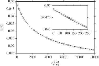
Figure 1: The decay of the free wobbling kink. Crosses: $|a(t)|$ as obtained from the direct numerical simulations of Eq.(1) with the initial conditions in the form $\phi=\tanh x+2a_{0}\operatorname{sech}x\tanh x$, $\phi_{t}=0$, with $a_{0}=0.05$. Solid curve: equation (34) with $|a(0)|=0.0492$. The inset shows the first 250 periods of oscillation; during this time the amplitude drops by less than $10\%$.

The equation (32) gives us the leading-order contributions to the frequency of the wobbling:

$$\omega=\omega_{0}\left[1-\tfrac{1}{2}v^{2}+\tfrac{1}{2}\operatorname{Re}\zeta\,|a|^{2}+{\mathcal{O}}\left(|a|^{4}\right)\right],$$ (35)

with $\operatorname{Re}\zeta<0$ as in (31). The $|a|^{2}$-term here is a nonlinear shift from the linear frequency $\omega_{0}=\sqrt{3}$. The $v^{2}$-term comes from the transverse Doppler effect. We could have obtained this term simply by calculating the wobbling frequency in the rest frame and then multiplying the result by the relativistic time-dilation factor $\sqrt{1-v^{2}}$ (which becomes $1-\tfrac{1}{2}v^{2}$ for small $v$).

III Conclusion

One result of this project is the uniform asymptotic expansion of the wobbling kink. In terms of the original variables, this expansion reads

$$\phi(x,t)=\tanh\left(\frac{1-3|a|^{2}}{\sqrt{1-v^{2}}}\xi\right)+a\operatorname{sech}\xi\tanh\xi e^{i\omega_{0}(t-v\xi)}+c.c.\\ +2|a|^{2}\operatorname{sech}^{2}\xi\tanh\xi+a^{2}f(\xi)e^{2i\omega_{0}(t-v\xi)}+c.c.+{\mathcal{O}}\left(|a|^{3}\right).$$ (36)

Here $\xi=x-vt$ and $f(\xi)$ is given by Eq.(25). The first term describes the “background”, stationary, kink with the width modified by the wobbling. [Note that we have incorporated two $X_{0}\operatorname{sech}^{2}X_{0}$ terms of the sum (21) into the width of the kink.] The second term is the wobbling mode itself; the third one accounts for further stationary deformation of the kink’s shape, and the last term represents the second-harmonic radiation from the wobbler.

Our second result is the amplitude equation (32) and the conclusion of the extreme longevity of the wobbling mode which follows from (32). In view of its anomalously long lifetime, the wobbling kink can be regarded as one of the fundamental nonlinear excitations of the $\phi^{4}$ theory, on par with the nonoscillatory kinks and breathers.

- (1) A. R. Bishop and T. Schneider (eds). Solitons and condensed matter physics. Springer-Verlag, Berlin, 1978; A.R. Bishop. Solitons and Physical Perturbations. In: Solitons in Action. Editors K. Lonngren and A. Scott. Academic Press, New York, 1978
- (2) R. Rajaraman, Solitons and Instantons. North-Holland, Amsterdam, 1982; N. Manton and P. Sutcliffe. Topological Solitons. Cambridge University Press, Cambridge, England, 2004
- (3) A. Vilenkin and E. P. S. Shellard. Cosmic Strings and Other Topological Defects. Cambridge University Press, Cambridge, England, 1994
- (4) S Aubry, J. Chem. Phys. 64 3392 (1976)
- (5) A. E. Kudryavtsev, JETP Lett. 22 82 (1975); Ablowitz M J, Kruskal M D, Ladik J F, SIAM J. Appl. Math. 36 428 (1979); Sugiyama T, Prog. Theor. Phys. 61 1550 (1979); Moshir M., Nucl. Phys. B 185 318 (1981); C A Wingate, SIAM J. Appl. Math. 43 120 (1983); Klein R, Hasenfratz W, Theodorakopoulos N, Wunderlich W, Ferroelectrics 26 721 (1980); D. K. Campbell, J. F. Schonfeld, and C. A. Wingate, Physica D 9 1 (1983); Belova T I, Kudryavtsev A E, Physica D 32 18 (1988); Anninos P, Oliveira S, Matzner R A, Phys. Rev. D 44 1147 (1991); Belova T I, Physics of Atomic Nuclei 58 124 (1995); Belova T I, Kudryavtsev A E, Uspekhi Fizicheskikh Nauk, 167 377 (1997)
- (6) B. S. Getmanov, JETP Lett. 24 291 (1976)
- (7) Belova T I, ZhETF 109 1090 (1996)
- (8) M J Rice and E J Mele, Solid State Commun. 35 487 (1980); M J Rice, Phys Rev B 28 3587 (1983)
- (9) H. Segur, J. Math. Phys. 24, 1439 (1983)
- (10) A.L. Sukstanskii and K.I. Primak, Phys Rev Lett 75 3029 (1995)
- (11) O M Kiselev, Russian J. Math. Phys. 5 29 (1997); Siberian Mathematical Journal 41 2 (2000)