El Niño Southern Oscillation as Sporadic Oscillations between Metastable States

Abstract.

The main objective of this article is to establish a new mechanism of the El Niño Southern Oscillation (ENSO), as a self-organizing and self-excitation system, with two highly coupled processes. The first is the oscillation between the two metastable warm (El Niño phase) and cold events (La Niña phase), and the second is the spatiotemporal oscillation of the sea surface temperature (SST) field. The interplay between these two processes gives rises the climate variability associated with the ENSO, leads to both the random and deterministic features of the ENSO, and defines a new natural feedback mechanism, which drives the sporadic oscillation of the ENSO. The new mechanism is rigorously derived using a dynamic transition theory developed recently by the authors, which has also been successfully applied to a wide range of problems in nonlinear sciences.

1. Introduction

This article is part of a research program initiated recently by the authors on dynamic transitions in geophysical fluid dynamics and climate dynamic. The main objective is to study the interannual low frequency variability of the atmospheric and oceanic flows, associated with typical sources of the climate variability, including the wind-driven (horizontal) and the thermohaline (vertical) circulations (THC) of the ocean, and the El Niño Southern Oscillation (ENSO). Their variability, independently and interactively, may play a significant role in climate changes, past and future.

ENSO is the known strongest interannual climate variability associated with strong atmosphere-ocean coupling, which has significant impacts on global climate. ENSO is in fact a phenomenon that warm events (El Niño phase) and clod events (La Niña phase) in the equatorial eastern Pacific SST anomaly, which are associated with persistent weakening or strengthening in the trade winds.

It is convenient and understandable to employ simplified coupled dynamical models to investigate some essential behaviors of ENSO dynamics; see among many others [24, 1, 6, 25, 19, 7, 18, 16, 17, 5, 23, 22, 21].

An interesting current debate is whether ENSO is best modeled as a stochastic or chaotic system - linear and noise-forced, or nonlinear oscillatory and unstable system [19]? It is obvious that a careful fundamental level examination of the problem is crucial. The main objective of this article is to address this fundamental question.

By establishing a rigorous mathematical theory on the formation of the Walker circulation over the tropics, we present in this article a new mechanism of the ENSO. Here we present a brief account of this new mechanism, and refer the readers to Section 5 for more precise description.

We show that interannual variability of ENSO is the interplay of two oscillation processes. The first is the oscillation between the metastable warm event (El Niño phase), normal event, and cold event (La Niña phase). We show that each metastable state has a basin of attraction, and the uncertainty of the initial states between these basins of attraction gives rise of the oscillation between these metastable states. The second is the spatiotemporal oscillation of the sea surface temperature (SST) field, which is mainly caused by the solar heating and the oceanic upwelling near Peru.

The interplay between these two processes give rises the inter-annual variability associated with the ENSO. On the one hand, the metastable states oscillation has direct influence on the SST, leading to 1) the intensification or weakening of the oceanic upwelling, and 2) the variation of the atmospheric Rayleigh number. Consequently, forcing the system to adjust to a different metastable phase, and to intensify/weaken the corresponding event. On the other hand, the oscillation of the SST has a direct influence on the atmospheric Rayleigh number, leading to a different El Niõ, La Niña and normal conditions.

This interplay The above mechanism of ENSO as an interplay of the two processes defines a new natural feedback mechanism, which drives the sporadic oscillation of the ENSO, and leads to both the random and deterministic features of the ENSO. The uncertainty is closely related to the fluctuations between the narrow basins of attractions of the corresponding metastable events, and the deterministic feature is represented by the deterministic modeling predicting the basins of attraction and the SST. Hence ENSO can be considered as a self-organizing and self-excitation system.

The main technical method is the dynamical transition theory developed recently by the authors. The main philosophy of the dynamic transition theory is to search for the full set of transition states, giving a complete characterization on stability and transition. The set of transition states –physical ”reality” – is represented by a local attractor. Following this philosophy, the theory is developed to identify the transition states and to classify them both dynamically and physically; see [13, 15] from application point of view of the theory.

With this theory, many longstanding phase transition problems are either solved or become more accessible. The modeling and the analysis with the applications of the theory to specific physical problems, on the one hand, provide verifications of existing experimental and theoretical studies, and, on the other hand, lead to various new physical predictions. For example, our study [12, 15, 14] of phase transitions of both liquid helium-3 and helium-4 leads not only to a theoretical understanding of the phase transitions to superfluidity observed by experiments, but also to such physical predictions as the existence of a new superfluid phase C for liquid helium-3. Although these predictions need yet to be verified experimentally, they certainly offer new insights to both theoretical and experimental studies for a better understanding of the underlying physical problems.

2. Atmospheric Model over the Tropics

Upwelling and zonal circulation over the tropics contains six convective cells, as shown in Figure 2.1. Usually the Walker circulation is referred to the Pacific cell over the equator, responsible for creating ocean upwelling off the coasts of Peru and Ecuador. It was discovered by Jacob Bjerknes in 1969 and was named after the English physicist Gilbert Walker, an early-20th-century director of British observatories in Indian, who discovered an indisputable link between periodic pressure variations in the Indian Ocean and the Pacific, which he termed the ”Southern Oscillation”.

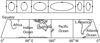
Figure 2.1. Global atmospheric Walker circulation over the tropics.

The Walker cell is of such importance that its behavior is a key factor giving rise to the El Niño (more precisely, the El Niño-Southern Oscillation (ENSO)) phenomenon. When the convective activity weakens or reverses, an El Niño phase takes place, causing the ocean surface to be warmer than average, reducing or terminating the upwelling of cold water. A particularly strong Walker circulation causes a La Niña event, resulting in cooler ocean temperature due to stronger upwelling; see Figure 2.2.

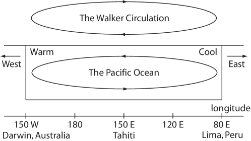
Figure 2.2. A schematic diagram of the Walker circulation at the equatorial Pacific Ocean, a main factor of the El Niño and the la Niña phenomena.

The atmospheric motion associated with the Walker circulation affects the loops on either side. Under normal years, the weather behaves as expected. But every few years, the winters becomes unusually warm or unusually cold, or the frequency of hurricanes increases or decreases. This entirely ocean-based cell is seen at the lower surface as easterly trade winds which drives the seawater and air warmed by sun moving towards the west. The western side of the equatorial Pacific is characterized by warm, wet low pressure weather, and the eastern side is characterized by cool, dry high pressure weather. The ocean is about 60 cm higher in the western Pacific as the result of this circulation. The air is returned at the upper surface to the east, and it now becomes much cooler and drier. An El Niño phase is characterized by a breakdown of this water and air cycle, resulting in relatively warm water and moist air in the eastern Pacific. Meanwhile, a La Niña phase is characterized by the strengthening of this cycle, resulting in much cooler water and drier air than the normal phase. During an El Niño or La Niña event, which occurs about every 3-6 years, the weather sets in for an indeterminate period.

It is then clear that the ENSO is a coupled atmospheric-ocean phenomena. The main objective of this section is to address the mechanism of atmospheric Walker circulations over the tropics from the dynamic transition point of view.

The atmospheric motion equations over the tropics are the Boussinesq equations restricted on $\theta=0$, where the meridional velocity component $u_{\theta}$ is set to zero, and the effect of the turbulent friction is taking into considering using the scaling law derived in [20]:

(2.1) $$\frac{\partial u_{\varphi}}{\partial t}=-(u\cdot\nabla)u_{\varphi}-\frac{u_{\varphi}u_{z}}{a}+\nu\left(\Delta u_{\varphi}+\frac{2}{a^{2}}\frac{\partial u_{z}}{\partial\varphi}-\frac{2u_{\varphi}}{a^{2}}\right)$$

$$\ \ \ \ -\sigma_{0}u_{\varphi}-2\Omega u_{z}-\frac{1}{\rho_{0}a}\frac{\partial p}{\partial\varphi},$$

$$\frac{\partial u_{z}}{\partial t}=-(u\cdot\nabla)u_{z}+\frac{u^{2}_{\varphi}}{a}+\nu\left(\Delta u_{z}-\frac{2}{a^{2}}\frac{\partial u_{\varphi}}{\partial\varphi}-\frac{2u_{z}}{a^{2}}\right)$$

$$\ \ \ \ -\sigma_{1}u_{z}+2\Omega u_{\varphi}-\frac{1}{\rho_{0}}\frac{\partial p}{\partial z}-(1-\alpha_{T}(T-T_{0}))g,$$

$$\frac{\partial T}{\partial t}=-(u\cdot\nabla)T+\kappa\Delta T,$$

$$\frac{1}{a}\frac{\partial u_{\varphi}}{\partial\varphi}+\frac{\partial u_{z}}{\partial z}=0.$$

Here $\sigma_{i}=C_{i}h^{2}$ ($i=0,1$) represent the turbulent friction, $a$ is the radius of the earth, the space domain is taken as $M=S^{1}_{a}\times(a,a+h)$ with $S^{1}_{a}$ being the one-dimensional circle with radius $a$, and

$$(u\cdot\nabla)=\frac{u_{\varphi}}{a}\frac{\partial}{\partial\varphi}+u_{z}\frac{\partial}{\partial z},\qquad\Delta=\frac{1}{a^{2}}\frac{\partial^{2}}{\partial\varphi^{2}}+\frac{\partial^{2}}{\partial z^{2}}.$$

For simplicity, we denote

$$(x_{1},x_{2})=(a\varphi,z),\qquad(u_{1},u_{2})=(u_{\varphi},u_{z}).$$

In atmospheric physics, the temperature $T_{1}$ at the tropopause $z=a+h$ is a constant. We take $T_{0}$ as the average on the lower surface $z=a$. To make the nondimensional form, let

$$x=hx^{\prime},\qquad t=h^{2}t^{\prime}/\kappa,\qquad u=\kappa u^{\prime}/h,$$

$$T=(T_{0}-T_{1})T^{\prime}+T_{0}-(T-T_{0})x^{\prime}_{2},$$

$$p=\kappa\nu\rho_{0}p^{\prime}/h^{2}-g\rho_{0}(hx^{\prime}_{2}+\alpha_{T}(T_{0}-T_{1})hx^{\prime 2}/2).$$

Also, we define the Rayleigh number, the Prandtl number and the scaling laws by

(2.2) $$R=\frac{\alpha_{T}g(T_{0}-T_{1})h^{3}}{\kappa\nu},\qquad\text{\rm Pr }=\frac{\nu}{\kappa},\qquad\delta_{i}=C_{i}h^{4}/\nu\quad(i=0,1).$$

Omitting the primes, the nondimensional form of (2.1) reads

(2.3) $$\frac{\partial u_{1}}{\partial t}=\text{Pr }\left[\Delta u_{1}+\frac{2}{r_{0}}\frac{\partial u_{2}}{\partial x_{1}}-\frac{2}{r_{0}}u_{1}-\delta_{0}u_{1}-\frac{\partial p}{\partial x_{1}}\right]$$

$$\ \ \ \ -\omega u_{2}-(u\cdot\nabla)u_{1}-\frac{1}{r_{0}}u_{1}u_{2},$$

$$\frac{\partial u_{2}}{\partial t}=\text{Pr }\left[\Delta u_{2}-\frac{2}{r_{0}}\frac{\partial u_{1}}{\partial x_{1}}-\frac{2}{r_{0}}u_{2}-\delta_{1}u_{2}+RT-\frac{\partial p}{\partial x_{2}}\right]$$

$$\ \ \ \ +\omega u_{1}-(u\cdot\nabla)u_{2}-\frac{1}{r_{0}}u^{2}_{1},$$

$$\frac{\partial T}{\partial t}=\Delta T+u_{2}-(u\cdot\nabla)T,$$

$$\frac{\partial u_{1}}{\partial x_{1}}+\frac{\partial u_{2}}{\partial x_{2}}=0,$$

where $(x_{1},x_{2})\in M=(0,2\pi r_{0})\times(r_{0},r_{0}+1)$, $\delta_{0}$ and $\delta_{1}$ are as in (2.2), $(u\cdot\nabla)$ and $\Delta$ as usual differential operators, and

(2.4) $$\omega=\frac{2\Omega h^{2}}{\kappa}.$$

The problem is supplemented with the natural periodic boundary condition in the $x_{1}$-direction, and the free-slip boundary condition on the top and bottom boundary:

(2.5) $$(u,T)(x_{1}+2\pi r_{0},x_{2},t)=(u,T)(x_{1},x_{2},t),$$

(2.6) $$\left\{\begin{aligned} &u_{2}=0,\ \frac{\partial u_{1}}{\partial x_{2}}=0,T=\varphi(x_{1})\qquad&&\text{at}\ x_{2}=r_{0},\\ &u_{2}=0,\ \frac{\partial u_{1}}{\partial x_{2}}=0,\ T=0\qquad&&\text{at}\ x_{2}=r_{0}+1.\end{aligned}\right.$$

Here $\varphi(x_{1})$ is the temperature deviation from the average $T_{0}$ on the equatorial surface and is periodic, i.e.,

$$\int^{2\pi r_{0}}_{0}\varphi(x_{1})dx_{1}=0\ \ \ \ \text{and }\ \varphi(x_{1})=\varphi(x_{1}+2\pi r_{0}).$$

The deviation $\varphi(x_{1})$ is mainly caused by a difference in the specific heat capacities between the sea water and land.

3. Walker Circulation under the Idealized Conditions

In an idealized case, the temperature deviation $\varphi$ vanishes. In this case, the study of transition of (2.3) is of special importance to understand the longitudinal circulation. Here, we are devoted to discuss the dynamic bifurcation of (2.3), the Walker cell structure of bifurcated solutions, and the convection scale under the idealized boundary condition

(3.1) $$\varphi(x_{1})=0\qquad\text{ for any }0\leq x_{1}\leq 2\pi r_{0}.$$

The following theorem provides a theoretical basis to understand the equatorial Walker circulation. The proof of this theorem follows the same method as given in [11], where similar results are obtained for the classical Bénard convection.

Theorem 3.1.

Under the idealized condition (3.1), the problem (2.3) with (2.5) and (2.6) undergoes a Type-I transition at the critical Rayleigh number $R=R_{c}$. More precisely, the following statements hold true:

• When the Rayleigh number $R\leq R_{c}$, the equilibrium solution $(u,T)=0$ is globally stable in the phase space $H$ defined by:

  $$H=\{(u,T)\in L^{2}(M)^{3}\ |\ \text{\rm div}u=0,u_{2}|_{x_{2}=r_{0},r_{0}+1}=0,(u,T)\ \text{satisfies}\ (\ref{10.41})\},$$

  where $L^{2}(M)$ stands for the square-integrable functions in $M$.

• When $R_{c}<R<R_{c}+\delta$ for some $\delta>0$, this problem bifurcates from $((u,T),R)=(0,R_{c})$ to an attractor ${\mathcal{A}}_{R}=S^{1}$, consisting of steady state solutions, which attracts $H\setminus\Gamma$ , where $\Gamma$ is the stable manifold of $(u,T)=0$ with codimension two.

• For each steady state solution $\psi_{R}=(u_{R},T_{R})\in{\mathcal{R}},u_{R}$ is topologically equivalent to the structure as shown in Figure 3.1.

• For any initial value $\psi_{0}=(u_{0},T_{0})\in H\setminus(\Gamma\cup E)$, there exists a time $t_{0}\geq 0$ such that for any $t>t_{0}$ the velocity field $u(t,\psi_{0})$ is topologically equivalent to the structure as shown in Figure 3.2 either (a) or (b), where $\psi=(u(t,\psi_{0}),T(t,\psi_{0}))$ is the solutions of the problem with $\psi(0)=\psi_{0}$, and

  $$E=\{(u,T)\in H|\ \int^{r_{0}+1}_{r_{0}}u_{1}dx_{2}=0\}.$$

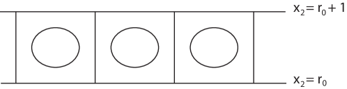
Figure 3.1. The cell structure of the steady state solutions in the bifurcated attractor ${\mathcal{A}}_{R}$.

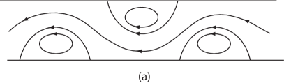
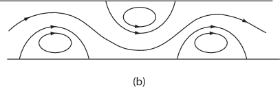
Figure 3.2. The Walker cell structure with the cells separated by a cross channel flow: (a) a westbound cross channel flow, and (b) an eastbound cross channel flow. This cross-channel flow pattern has the same topological structure as the Walker circulation over the tropics and the Branstator-Kushnir waves in the atmospheric dynamics [2, 8].

A few remarks are now in order:

First, in a more realized case where $T=T_{0}+\varphi(x_{1})$ at $x_{2}=r_{0}$, the temperature deviation $\varphi(x_{1})$ is small in comparison with the average temperature gradient $T_{0}-T_{1}$. Therefore, the more realistic case can be considered as a perturbation of the idealized case.

Second, mathematically, the conclusion that ${\mathcal{A}}_{R}=S^{1}$ consisting of steady state solutions is derived from the invariance of (2.3) under a translation $x_{1}\rightarrow x_{1}+\alpha$. It implies that for any two solutions $\psi_{1},\psi_{2}\in{\mathcal{A}}_{R}$, they are the same up to a phase angle $\alpha$ in the longitude, namely

$$\psi_{2}(x_{1},x_{2})=\psi_{1}(x_{1}+\alpha,x_{2}),\ \text{for\ some}\ \alpha\in[0,2\pi r_{0}].$$

For the idealized case, this conclusion is nature as the equator is treated as homogeneous.

In addition, Assertion (2) amounts to saying that as the initial value $\psi_{0}$ varies, i.e., an external perturbation is applied, the rolls of the Walker circulation will be translated by a phase angle $\alpha$. This behavior is termed as the translation oscillation, which can be used to explain the ENSO phenomenon for the idealized circumstance.

Third, when a deviation $\varphi(x_{1})$ is present, the translation symmetry is broken, and consequently, the bifurcated attractor ${\mathcal{A}}_{R}$ consists of isolated equilibrium solutions instead of a circle $S^{1}$. Thus, the mechanism of the ENSO will be explained as state exchanges between these equilibrium solutions in ${\mathcal{A}}_{R}$, which are metastable. We shall address this point in detail later.

Fourth, by the structural stability theorems in [10], we see from Assertion (4) that the roll structures illustrated by Figure 3.2 (a) and (b) are structurally stable. Hence, for a deviation perturbation $\varphi(x_{1})$, these structures are not destroyed, providing a realistic characterization of the Walker circulation.

Fifth, in Assertion (3), these rolls in the bifurcated solutions are closed. However, under some external perturbation, a cross channel flow appears which separates the rolls apart, and globally transports heat between them.

Sixth, it is then classical [11, 9, 3, 4] to show that the critical Rayleigh number is given by

(3.2) $$R_{c}=\min\limits_{\alpha^{2}}\left[(\alpha^{2}+\pi^{2})\delta_{1}+\frac{(\alpha^{2}+\pi^{2})^{3}+\pi^{2}(\alpha^{2}+\pi^{2})\delta_{0}}{\alpha^{2}}\right].$$

Let $g(x)=(x+\pi^{2})\delta_{1}+((x+\pi^{2})^{3}+\pi^{2}(x+\pi^{2})\delta_{0})/x$. Then, $x_{c}=\alpha^{2}_{c}$ satisfies $g^{\prime}(x)=0$. Thus we get

(3.3) $$\delta_{1}\alpha^{4}_{c}-(\alpha^{2}_{c}+\pi^{2})^{3}-\pi^{2}(\alpha^{2}_{c}+\pi^{2})\delta_{0}+3\alpha^{2}_{c}(\alpha^{2}_{c}+\pi^{2})^{2}+\pi^{2}\alpha^{2}_{c}\delta_{0}=0.$$

We assume that $\delta_{1}>\delta_{0}$ for $h\neq 0$. By $\alpha^{2}_{c}=\pi^{2}/L^{2}_{c}$, when $h$ is large, $\delta_{1}\gg 1$ and $\delta_{1}\gg\delta_{0}$, from (3.2) and (3.3) we derive that

(3.4) $$\alpha^{4}_{c}\cong\frac{\pi^{4}(\pi^{2}+\delta_{0})}{\delta_{1}},$$

(3.5) $$L^{2}_{c}\cong\delta^{{1}/{2}}_{1}/(\pi^{2}+\delta_{0})^{{1}/{2}},$$

(3.6) $$R_{c}\cong\pi^{2}\delta_{1}+\pi^{2}\delta_{0}L^{2}_{c},$$

These formulas (3.4)-(3.6) are very useful in studying large-scale convection motion, as shown in the next section.

4. Walker circulation under natural conditions

4.1. Physical parameters and effects of the turbulent friction terms

It is known that air properties vary with the temperature and pressure. The table below lists some common properties of air: density, kinematic viscosity, thermal diffusivity, expansion coefficient and the Prandtl number for temperatures between-$100^{\circ}$C and $100^{\circ}$C.

$\begin{aligned} &\text{Temperature}\\ &\ \ t\\ &(^{\circ}C)\end{aligned}$	$\begin{aligned} &\text{Density}\\ &\ \ \rho\\ &(\text{kg/m}^{3})\end{aligned}$	$\begin{aligned} &\text{Kinematic}\\ &\text{viscosity}\\ &\ \ \nu\\ &(\text{m}^{2}/\text{s})\times 10^{-6}\end{aligned}$	$\begin{aligned} &\text{Thermal}\\ &\text{Diffusivity}\\ &\ \ \kappa\\ &(\text{m}^{2}/\text{s})\times 10^{-6}\end{aligned}$	$\begin{aligned} &\text{Expansion}\\ &\text{coefficient}\\ &\ \ a\\ &(1/\text{k})\times 10^{-3}\end{aligned}$	$\begin{aligned} &\text{Prandtl}\\ &\text{number}\\ &\ \ \text{Pr }\end{aligned}$
-100	1.980	5.95	8.4	5.82	0.74
-50	1.534	9.55	13.17	4.51	0.725
0	1.293	13.30	18.60	3.67	0.715
20	1.205	15.11	21.19	3.40	0.713
40	1.127	16.97	23.87	3.20	0.711
60	1.067	18.90	26.66	3.00	0.709
80	1.000	20.94	29.58	2.83	0.708
100	0.946	23.06	32.8	2.68	0.703

The average temperature over the equator is about $20\sim 30^{\circ}$C. Based on the data in Table 4.1, we take a set of physical parameters of air for the Walker circulation as follows:

$$\nu=1.6\times 10^{-5}\text{m}^{2}/\text{s},\ \ \ \ \kappa=2.25\times 10^{-5}\text{m}^{2}/\text{s},$$

$$\alpha_{T}=3.3\times 10^{-3}/{}^{\circ}C,\ \ \ \ \text{Pr }=0.71.$$

The height $h$ of the troposphere is taken by

$$h=8\times 10^{3}\text{m}.$$

Thus, the Rayleigh number for the equatorial atmosphere is

(4.1) $$R=\frac{g\alpha_{T}(T_{0}-T_{1})}{\kappa\nu}h^{3}=3.6\times 10^{19}(T_{0}-T_{1})/{}^{\circ}C.$$

In the classical theory, we have the critical Rayleigh number

(4.2) $$R_{c}=\min\limits_{\alpha^{2}}\frac{(\alpha^{2}+\pi^{2})^{3}}{\alpha^{2}}=\frac{27}{4}\pi^{4}=675,$$

and the convective scale

(4.3) $$L^{2}_{c}=\pi^{2}/\alpha^{2}_{c}=2.$$

Namely, the diameter of convective roll is

$$d=L_{c}\times h=20\text{km}.$$

However, based on atmospheric observations, there are six cells overall tropics, and it shows that the real convective scale is about

(4.4) $$L=\frac{a\pi}{3}=6600\text{ km }.$$

As a comparison, the values (4.2) and (4.3) from the classical theory are too small to match the realistic data given in (4.1) and (4.4).

We use (3.4)-(3.6) to discuss this problem. With the values in (4.1) and (4.4), we take

(4.5) $$\delta_{1}=2.7\times 10^{20},\ \ \ \ \delta_{0}=3.5\times 10^{8}.$$

In comparison with (2.2), for air, the constants $C_{0}$ and $C_{1}$ take the following values

$$C_{0}=1.37\times 10^{-12}\ m^{-2}\cdot s^{-1},\qquad C_{1}=1.05\ m^{-2}\cdot s^{-1}.$$

Then, the convective scale $L_{c}$ in (3.5) takes the value

(4.6) $$L_{c}=[\delta_{1}/\delta_{0}]^{{1}/{4}}h=7500\text{km},$$

which is slightly bigger than the realistic value $L\cong 6300\text{km}$. And, the critical Rayleigh number in (3.6) takes

$$R_{c}\cong\pi^{2}\delta_{1}+\pi^{2}\delta_{0}L^{2}_{c}\cong 2.7\times 10^{21}.$$

Thus, the critical temperature difference is

(4.7) $$\Delta T_{c}\cong 60^{\circ}C,$$

which is realistic, although it is slightly smaller than the realistic temperature difference on the equator.

However, with the classical theory with no friction terms, the critical values would be $L_{c}\cong 20km$ and $\Delta T_{c}\cong 10^{-17\circ}C$, which are certainly unrealistic.

4.2. Transition in natural conditions

We now return the natural boundary condition

$$\varphi(x_{1})\not\equiv 0.$$

In this case, equations (2.3) admits a steady state solution

(4.8) $$\tilde{\psi}=(V,J),\ \ \ \ (V=(V_{1},V_{2})).$$

Consider the deviation from this basic state:

$$u\rightarrow u+V,\ \ \ \ T\rightarrow T+J.$$

Then (2.3) becomes

(4.9) $$\frac{\partial u_{1}}{\partial t}+(u\cdot\nabla)u_{1}+\frac{u_{1}u_{2}}{r_{0}}=\text{Pr }[\Delta u_{1}-\delta^{\prime}_{0}u_{1}-\frac{\partial p}{\partial x_{1}}]$$

$$\ \ \ \ -(u\cdot\nabla)u_{1}-(u\cdot\nabla)V_{1}-\frac{V_{1}}{r_{0}}u_{2}-\frac{V_{2}}{r_{0}}u_{1},$$

$$\frac{\partial u_{2}}{\partial t}+(u\cdot\nabla)u_{2}-\frac{u^{2}_{1}}{r_{0}}=\text{Pr }[\Delta u_{2}-\delta^{\prime}_{1}u_{2}+RT-\frac{\partial p}{\partial x_{2}}]$$

$$\ \ \ \ -(u\cdot\nabla)u_{2}-(u\cdot\nabla)V_{2}+\frac{2V_{1}}{r_{0}}u_{1},$$

$$\frac{\partial T}{\partial t}+(u\cdot\nabla)T=\Delta T+u_{2}-(u\cdot\nabla)J-(u\cdot\nabla)T,$$

$$\text{div}u=0.$$

The boundary conditions are the free-free boundary conditions given by

(4.10) $$(u,T)\ \text{is\ periodic\ in}\ x_{1}-\text{direction},$$

$$T=0,u_{2}=0,\frac{\partial u_{1}}{\partial x_{2}}=0\ \text{at}\ x_{2}=r_{0},r_{0}+1.$$

It is known that $|\varphi(x_{1})|$, with $\Delta T=T_{0}-T_{1}\cong 100^{\circ}C$ as unit, is small. Hence, the steady state solution $(V,J)$ is also small:

$$\|(V,J)\|_{L^{2}}=\varepsilon\ll 1.$$

Thus, (4.9) is a perturbated equation of (2.3).

Since perturbation terms involving $(V,J)$ are not invariant under the zonal translation (in the $x_{1}$-direction), for general small functions $\varphi(x_{1})\neq 0$, the first eigenvalues of (4.9) are (real or complex) simple, and by the perturbation theorems in [9], all eigenvalues of linearized equation of (4.9) satisfy the following principle of exchange of stability (PES):

$$\text{Re}\beta^{\varepsilon}_{i}(R)\left\{\begin{aligned} &<0&&\text{ for }R<R^{\varepsilon}_{c},\\ &=0&&\text{ for }R=R^{\varepsilon}_{c},\\ &>0&&\text{ for }R>R^{\varepsilon}_{c},\end{aligned}\right. \text{ for any }1\leq i\leq m,$$

$$\text{Re}\beta^{e}_{j}(R^{\varepsilon}_{c})<0 \text{ for any }j\geq m+1,$$

where $m=1$ as $\beta^{\varepsilon}_{1}(R)$ is real, $m=2$ as $\beta^{\varepsilon}_{1}(R)$ is complex near $R^{\varepsilon}_{c}$, and $R^{\varepsilon}_{c}$ is the critical Rayleigh number of perturbed system (4.9).

The following two theorems follow directly from Theorem 3.1 and the perturbation theorems in [9].

Theorem 4.1.

Let $\beta^{\varepsilon}_{1}(R)$ near $R=R^{\varepsilon}_{c}$ be a real eigenvalue. Then the system (4.9) has a transition at $R=R^{\varepsilon}_{c}$, which is either mixed (Type-III) or continuous (Type-I), depending on the temperature deviation $\varphi(x_{1})$. Moreover, we have the following assertions:

• If the transition is Type-I, then as $R^{\varepsilon}_{c}<R<R^{\varepsilon}_{c}+\delta$ for some $\delta>0$, the system bifurcates at $R^{\varepsilon}_{c}$ to exactly two steady state solutions $\psi_{1}$ and $\psi_{2}$ in $H$, which are attractors. In particular, space $H$ can be decomposed into two open sets $U_{1},U_{2}$:

  $$H=\bar{U}_{1}+\bar{U}_{2},\ \ \ \ U_{1}\cap U_{2}=\phi,\ \ \ \ \psi=0\in\partial U_{1}\cap\partial U_{2},$$

  such that $\psi_{i}\in U_{i}$ $(i=1,2)$, and $\psi_{i}$ attracts $U_{i}$.

• If the transition is Type-III, then there is a saddle-node bifurcation at $R=R^{*}$ with $R^{*}<R^{\varepsilon}_{c}$ such that the following statements hold true:

  • if $R^{*}<R<R^{\varepsilon}_{c}+\delta$ with $R\neq R^{\varepsilon}_{c}$, the system has two steady state solutions $\psi^{R}_{+}$ and $\psi^{R}_{-}$ which are attractors, as shown in Figure 5.3, such that

    $$\psi^{R}_{+}=0\qquad\text{ for }R^{*}<R<R^{\varepsilon}_{c}.$$

  • There is an open set $U\subset H$ with $0\in U$ which can be decomposed into two disjoint open sets $\bar{U}=\bar{U}^{R}_{+}+\bar{U}^{R}_{-}$ with $\psi^{R}_{\pm}\in U^{R}_{\pm}$ and $\psi^{R}_{\pm}$ attracts $U^{R}_{\pm}$.

• For any initial value $\psi_{0}=(u_{0},T_{0})\in U^{R}_{-}$ for $R>R^{\ast}$ or $\psi_{0}=(u_{0},T_{0})\in U^{R}_{+}$ for $R>R^{\varepsilon}_{c}$, there exists a time $t_{0}\geq 0$ such that for any $t>t_{0}$ the velocity field $u(t,\psi_{0})$ is topologically equivalent to the structure as shown in Figure 3.2 either (a) or (b), where $\psi=(u(t,\psi_{0}),T(t,\psi_{0}))$ is the solutions of the problem with $\psi(0)=\psi_{0}$.

Theorem 4.2.

Let $\beta^{\varepsilon}_{1}(R)$ be complex near $R=R^{\varepsilon}_{c}$. Then the system (4.9) bifurcates from $(\psi,R)=(0,R^{\varepsilon}_{c})$ to a periodic solution $\psi_{R}(t)$ on $R^{\varepsilon}_{c}<R$, which is an attractor, and $\psi_{R}(t)$ can be expressed as

(4.11) $$\psi_{R}(t)=A_{R}(\cos\rho t\psi_{1}+\sin\rho t\tilde{\psi}_{1})+o(|A_{R}|,\varepsilon),$$

where $A_{R}=\alpha(R-R^{\varepsilon}_{c}),\alpha$ and $\rho$ are constants depending on $\varphi(x_{1})$, and $\psi_{1},\tilde{\psi}_{1}$ are first eigenfunctions of linearized equations of (2.3).

A few remarks are now in order.

First, Theorems 3.1, 4.1 and 4.2 provide the possible dynamical behaviors for the zonal atmospheric circulation over the tropics. Theorem 3.1 describes the translation oscillation, and does not represent a realistic explanation to the ENSO.

Second, the periodic solution (4.11) characterizes a roll pattern translating with a constant velocity over the equator, eastward or westward, as shown in Figure 4.1 (a) and (b) The time-periodic oscillation obtained in Theorem 4.2 does not represent the typical oscillation in the ENSO phenomena, as the Walker circulation does not obey this zonal translational oscillation.

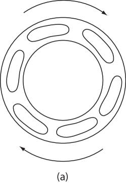
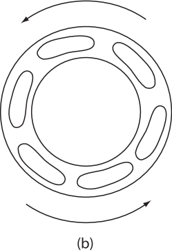
Figure 4.1. Time-periodic translation of the Walker circulation pattern; (a) an eastward translation, (b) a westward translation.

Third, Theorem 4.1 characterizes the oscillation between metastable states, The oscillation between the metastable states in Theorem 4.1 can be either Type-I or Type-III, depending on the number

$$b=<G(\Psi_{1}),\Psi^{*}_{1}>,$$

where $\Psi_{1}$ is the first eigenvector of the linearized equation of (4.9) at $R=R^{\varepsilon}_{c}$, $\Psi^{*}$ is the corresponding first eigenvector of the adjoint linearized problem, and $G$ represents the nonlinear terms in (4.9).

Namely, if $b\neq 0$, the transition is Type-III and if $b=0$, the transition is Type-I. From mathematical viewpoint, for almost all functions $\varphi$, $b\neq 0$. Hence, the case where $b\neq 0$, consequently the Type-III transition in Theorem 4.1, is generic. In other words, the Type-III transition derived in this theorem provides a correct oscillation mechanism of the ENSO between two metastable El Niño and La Niña events, and we shall explore this point of view in the next section in detail.

5. Metastable Oscillation Theory of ENSO

It is well known that the Walker cell at the equatorial Pacific Ocean is closely related to the ENSO phenomenon. Its behavior is the key to the understanding of ENSO.

Southern Oscillation Phenomenon. The Southern Oscillation Index (SOI) gives a simple measure of the strength and phase of the Southern Oscillation, and indicates the state of the Walker circulation. The SOI is defined by the pressure difference between Tahiti and Darwin. When the Walker circulation enters its El Niño phase, the SOI is strongly negative; when it is in the La Niña phase, the SOI is strongly positive; and in the normal state the SOI is small; see Figure 5.1.

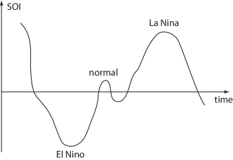
Figure 5.1. SOI indicates the state of the Walker circulation.

This point can be further examined by further observational data of SOI as shown in Figure 5.2. In the SOI diagram, we observe that there are two groups of oscillations: the relatively large amplitude fluctuation and the relatively small amplitude fluctuation. The large one occurred in 1950-1951, 1955-1956, and 1974-1975 for positive SOI higher than 13, in 1965-1966, 1972-1973, 1977-1978, 1981-1982, and 1987-1988 for negative SOI lower than -12. The small one with SOI between-8 to 8 appeared in other years.

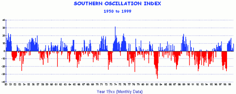
Figure 5.2. SOI diagram, adopted from Web: BOM-Monitoring Climate-Climate variability and El Niño.

El Niño and La Niña States. The non-homogeneous temperature distribution shows that the locations of the cells over the tropics are relatively fixed. This suggests that the homogeneous case as described by Theorem 3.1 is not a valid description of the realistic situation. In addition, the translation oscillation formation, suggest in Theorem 4.2, does not describe the ENSO either.

Hence the nature theory for the atmospheric circulation over the tropics associated with the Walker circulation and the ENSO is given by Theorem 4.1. It is known that the steady state solutions of (2.3) can be written as

(5.1) $$\tilde{\psi}+\psi_{R},$$

where $\tilde{\psi}=(V,J)$ is the steady state solution given by (4.8), and $\psi_{R}^{\pm}$ are the stable equilibria of (4.9), derived in Theorem 4.1. In fact, the ENSO phenomenon can be explained as the transition between the two metastable steady state solutions $\tilde{\psi}+\psi_{R}^{\pm}$.

Theorem 4.1 amounts to saying that for a mixed transition, there are two critical Rayleigh numbers $R^{*}$ and $R^{\varepsilon}_{c}$, with $R^{*}<R^{\varepsilon}_{c}$, where $R^{\ast}\cong R_{c}\cong 2.7\times 10^{21}$. At $R=R^{*}$, the equation (4.9) has a saddle-node bifurcation, and at $R=R^{\varepsilon}_{c}$ has the normal transition, as shown in Figure 5.3. When the Rayleigh number $R$ is less than $R^{*}$, i.e. $R<R^{*}$, the system (2.3) has only one stable steady state solution $\tilde{\psi}=(V,J)$ as in (4.8) which attracts $H$. When $R^{*}<R<R^{\varepsilon}_{c}$, this system has two stable equilibriums

(5.2) $$\tilde{\psi}\in U^{R}_{+},\ \ \ \ \text{and}\ \ \ \ \tilde{\psi}+\psi^{-}_{R}\in U^{R}_{-},\ \ \ \ \text{for}\ \ \ \ R^{*}<R<R^{\varepsilon}_{c},$$

where $U^{R}_{+}$, $U^{R}_{-}\subset H$ are basins of attraction of $\tilde{\psi}$ and $\tilde{\psi}+\psi^{-}_{R}$. And when $R^{\varepsilon}_{c}<R$, this system has also two stable equilibriums

(5.3) $$\tilde{\psi}+\psi^{-}_{R}\in U^{R}_{-}\ \ \ \ \text{and}\ \ \ \ \tilde{\psi}+\psi^{+}_{R}\in U^{R}_{+}\ \ \ \ \text{for}\ R^{*}_{c}<R,$$

with $U^{R}_{-}$ and $U^{R}_{+}$ are their basins of attraction.

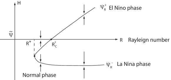
Figure 5.3. The transition diagram for the equatorial motion equations (2.3), $R^{*}$ is the saddle-node bifurcation point, $R^{\varepsilon}_{c}$ is the first critical Rayleigh number.

Since the problem (2.3) with a natural boundary condition is a perturbation for the idealized condition, $\tilde{\psi}=(V,J)$ is small, and the velocity field $V$ is almost zero. Hence the equilibrium

$$\Psi^{+}_{R}=\left\{\begin{aligned} &\tilde{\psi}&&\text{ for }R<R^{\ast}_{c},\\ &\tilde{\psi}+\psi^{+}_{R}&&\text{ for }R>R^{\ast}_{c},\end{aligned}\right.$$

represents the El Niño phase, and the equilibrium

$$\Psi^{-}_{R}=\tilde{\psi}+\psi^{-}_{R}$$

represents the normal phase for $R^{\ast}<R<R^{\ast}_{c}$, and the La Niña phase for $R^{\ast}_{c}<R$. It is clear that both $\Psi^{\pm}_{R}$ are metastable, with $U^{\pm}_{R}$ as their basins of attractions respectively.

Oscillation Mechanism of ENSO. The above theoretical studies suggest that ENSO is the interplay between two oscillation processes. The first is the oscillation between the metastable warm event (El Niño phase, represented by $\Psi^{+}_{R}$) and cold event (La Niña phase, represented by $\Psi_{R}^{-}$). The second oscillation is the oscillation of the Rayleigh number caused essentially by the some spatiotemporal oscillation of the sea surface temperature (SST) field.

Here we present a brief schematic description on the interplay between these two oscillation processes of the ENSO, based on the saddle-node transition diagram in Figure 5.3, rigorously proved in Theorem 4.1.

We start with three physical conclusions:

• We observe that as $R$ decreases, the normal and the La Niña phase $\Psi^{-}_{R}$ weakens and its basin of attraction shrinks (to zero as $R$ approaches to $R^{\ast}$).

• As $R$ increases in the interval $R^{\varepsilon}_{c}<R$, the strength of the El Niño phase increases. As $R$ increases in $(R^{\ast},R^{\varepsilon}_{c})$, the basin of attraction of the El Niño phase shrinks. In particular, near $R^{\varepsilon}_{c}$, the El Niño phase is close to the interaction of the two basins of attraction of the El Niño and La Niña phase; consequently, forcing the transition from the El Niño phase to the La Niña phase.

• Also, we see that as the El Niño event $\Psi^{+}_{R}$ intensifies, the SST increases, and as the normal and La Niña event $\Psi^{-}_{R}$ intensifies, the SST decreases.

From the above three physical conclusions, we obtain the following new mechanism of the ENSO oscillation process:

• When $R^{\ast}<R<R^{\varepsilon}_{c}$, $\Psi^{-}_{R}$ represents the normal condition, and the corresponding upwelling near Peru leads to the decreasing of the SST, and leads to $R$ approaching $R^{\ast}$. On the other hand, near $R^{\ast}$, the basin of attraction of the normal condition $\Psi^{-}_{R}$ shrinks, and due to the uncertainty of the initial data, the system can undergo a dynamic transition near $R^{\ast}$ toward to the El Niño phase $\Psi^{+}_{R}$.

• For the El Niño phase $\Psi^{+}_{R}=\tilde{\psi}$ near $R^{\ast}$, however, the velocity $V$ is small, and SST will increases due to the solar heating, which can not be transported away by weak oceanic currents without upwelling. Hence the corresponding Rayleigh number $R$ increases, and the El Niño phase intensifies. When the Rayleigh number approaches to the critical value $R^{\varepsilon}_{c}$, with high probability, the system undergoes a metastable transition from the El Niño phase to either the normal phase or the La Niña phase depending on the Rayleigh number $R$ and the the strength of the phase $\Psi^{-}_{R}$.

• With delaying effect, strong El Niño and La Niña occur at the Rayleigh number $R$ larger than the critical number $R^{\varepsilon}_{c}$, and the system will repeat the process described in items I-II above.

In summary, this new mechanism of ENSO as an interplay of the two processes leads to both the random and deterministic features of the ENSO, and defines a new natural feedback mechanism, which drives the sporadic oscillation of the ENSO. The randomness is closely related to the uncertainty/fluctuations of the initial data between the narrow basins of attractions of the corresponding metastable events, and the deterministic feature is represented by a deterministic coupled atmospheric and oceanic model predicting the basins of attraction and the SST. It is hoped this mechanism based on a rigorous mathematical theory could lead to a better understanding and prediction of the ENSO phenomena.

References

- [1] D. S. Battisti and A. C. Hirst, Interannual variability in a tropical atmosphere-ocean model. influence of the basic state, ocean geometry and nonlinearity, J. Atmos. Sci., 46 (1989), pp. 1687–1712.
- [2] G. W. Branstator, A striking example of the atmosphere’s leading traveling pattern, J. Atmos. Sci., 44 (1987), pp. 2310–2323.
- [3] S. Chandrasekhar, Hydrodynamic and Hydromagnetic Stability, Dover Publications, Inc., 1981.
- [4] P. Drazin and W. Reid, Hydrodynamic Stability, Cambridge University Press, 1981.
- [5] M. Ghil, Is our climate stable? bifurcations, transitions and oscillations in climate dynamics, in science for survival and sustainable development, v. i. keilis-borok and m. s nchez sorondo (eds.), pontifical academy of sciences, vatican city, (2000), pp. 163–184.
- [6] F. F. Jin, Tropical ocean-atmosphere interaction, the pacific cold tongue, and the el ni o southern oscillation, Science, 274 (1996), pp. 76–78.
- [7] F. F. Jin, D. Neelin, and M. Ghil, El niño/southern oscillation and the annual cycle: subharmonic frequency locking and aperiodicity, Physica D, 98 (1996), pp. 442–465.
- [8] Y. Kushnir, Retrograding wintertime low-frequency disturbances over the north pacific ocean, J. Atmos. Sci., 44 (1987), pp. 2727–2742.
- [9] T. Ma and S. Wang, Bifurcation theory and applications, vol. 53 of World Scientific Series on Nonlinear Science. Series A: Monographs and Treatises, World Scientific Publishing Co. Pte. Ltd., Hackensack, NJ, 2005.
- [10] , Geometric theory of incompressible flows with applications to fluid dynamics, vol. 119 of Mathematical Surveys and Monographs, American Mathematical Society, Providence, RI, 2005.
- [11] , Rayleigh-Bénard convection: dynamics and structure in the physical space, Commun. Math. Sci., 5 (2007), pp. 553–574.
- [12] , Dynamic model and phase transitions for liquid helium, Journal of Mathematical Physics, 49:073304 (2008), pp. 1–18.
- [13] , Dynamic phase transition theory in PVT systems, Indiana University Mathematics Journal, to appear; see also Arxiv: 0712.3713, (2008).
- [14] , Phase transition and separation for mixture of liquid he-3 and he-4, in a special issue dedicated to the legacy of landau, EJTP, (2008).
- [15] , Superfluidity of helium-3, Physica A: Statistical Mechanics and its Applications, 387:24 (2008), pp. 6013–6031.
- [16] J. D. Neelin, A hybrid coupled general circulation model for el niño studies, J. Atmos. Sci., 47 (1990), pp. 674–693.
- [17] , The slow sea surface temperature mode and the fast-wave limit: Analytic theory for tropical interannual oscillations and experiments in a hybrid coupled model, J. Atmos. Sci., 48 (1990), pp. 584–606.
- [18] J. D. Neelin, D. S. Battisti, A. C. Hirst, F.-F. Jin, Y. Wakata, T. Yamagata, and S. E. Zebiak, Enso theory, J. Geophys. Res., 103 (1998), p. 14261 14290.
- [19] S. G. Philander and A. Fedorov, Is el niño sporadic or cyclic?, Annu. Rev. Earth Planet. Sci., 31 (2003), p. 579 594.
- [20] M. L. Salby, Fundamentals of Atmospheric Physics, Academic Press, 1996.
- [21] R. M. Samelson, Time-periodic flows in geophysical and classical fluid dynamics. in: Handbook of numerical analysis, special volume on computational methods for the ocean and the atmosphere. r. temam and j. tribbia, eds. elsevier, new york. to appear, (2008).
- [22] P. D. Sardeshmukh, G. P. Compo, and C. Penland, Changes of probability associated with el niño, Journal of Climate, (2000), p. 4268 4286.
- [23] E. K. Schneider, B. P. Kirtman, D. G. DeWitt, A. Rosati, L. Ji, and J. J. Tribbia, Retrospective enso forecasts: Sensitivity to atmospheric model and ocean resolution, Monthly Weather Review, 131:12 (2003), pp. 3038–3060.
- [24] P. S. Schopf and M. J. Suarez, Vacillations in a coupled ocean-atmosphere model, J. Atmos. Sci., 45 (1987), pp. 549–566.
- [25] S. E. Zebiak and M. A. Cane, A model el ni o southern oscillation, Mon. Wea. Rev., 115 (1987), p. 2262 2278.