Iterative Solution of the Quasicontinuum Equilibrium Equations with Continuation

Abstract.

We give an analysis of a continuation algorithm for the numerical solution of the force-based quasicontinuum equations. The approximate solution of the force-based quasicontinuum equations is computed by an iterative method using an energy-based quasicontinuum approximation as the preconditioner.

The analysis presented in this paper is used to determine an efficient strategy for the parameter step size and number of iterations at each parameter value to achieve a solution to a required tolerance. We present computational results for the deformation of a Lennard-Jones chain under tension to demonstrate the necessity of carefully applying continuation to ensure that the computed solution remains in the domain of convergence of the iterative method as the parameter is increased. These results exhibit fracture before the actual load limit if the parameter step size is too large.

1. Introduction

Quasicontinuum (QC) approximations reduce the computational complexity of a material simulation by reducing the degrees of freedom used to describe a configuration of atoms and by giving approximate equilibrium equations on the reduced degrees of freedom [14, 15, 5, 21, 20, 11, 25, 13, 9, 10, 18, 23, 16, 6, 24, 7]. For crystalline materials, there are typically a few small regions with highly non-uniform structure caused by defects in the material which are surrounded by large regions where the local environment of atoms varies slowly. The idea of QC is to replace these slowly varying regions with a continuum model and couple it directly to the atomistic model surrounding the defects. The material’s position is described by a set of representative atoms that are in one-to-one correspondence with the lattice atoms in the atomistic regions but reduce the degrees of freedom in the continuum regions.

Quasi-static computations in material simulations explore mechanical response under slow external loading by fully relaxing the material at each step of a parameterized path of external conditions. Such simulations can model nano-indentation, stress-induced phase transformations, and many other material processes. The characteristic feature when using this technique is that the process to be modeled occurs slowly enough that dynamics are assumed to play no role in determining the relaxed state. This paper focuses on applying continuation techniques [4, 12, 8] to the nonlinear equilibrium equations of the force-based quasicontinuum approximation (QCF).

1.1. Choosing a Quasicontinuum Approximation

There are many choices available for the interaction among the representative atoms, especially between those in the atomistic and continuum regions, which has led to the development of a variety of quasicontinuum approximations. Criteria for determining a good choice of approximation for a given problem are still being developed. Algorithmic simplicity and efficiency is certainly important for implementation and application, but concerns about accuracy have led to the search for consistent schemes. Since the forces on all of the atoms in a uniformly strained lattice are zero, we define a quasicontinuum approximation to be consistent if there are no forces on the representative atoms for a lattice that has been deformed by a uniform strain. We note that the atomistic to continuum interface is typically where consistency fails for a QC approximation [7, 18, 24, 9] as is the case for the original QC method [25].

For static problems, QCF is an attractive choice for quasicontinuum approximation because it is a consistent scheme [7, 18] that is algorithmically simple: the force on each representative atom is given by either an atomistic calculation or a continuum finite element calculation. The algorithmic simplicity of the force-based quasicontinuum method has allowed it to be implemented with adaptive mesh refinement and atomistic to continuum model selection algorithms  [18, 6, 1, 2, 3, 22, 19]. The trade-off for the consistency and algorithmic simplicity of QCF is that it does not give a conservative force field, although it is close to a conservative field [7]. Thus, QCF is a method to approximate forces, rather than a method to approximate the energy.

Quasicontinuum energies have been proposed that utilize special energies for atoms in an interfacial region [24, 9], and corresponding conditions for consistency have been satisfied for planar interfaces [9]. However, there is currently no known consistent quasicontinuum energy that allows general nonplanar atomistic to continuum interfaces and mesh coarsening in the continuum region (other than the computationally intensive constrained quasicontinuum energy discussed in Section 2.2). We will, however, investigate the use of quasicontinuum energies as preconditioners for the force-based quasicontinuum approximation.

1.2. Solving Equilibrium Equations by Continuation

Our goal is to efficiently approximate the solution $\mathbf{z}(s)$ to the QCF equilibrium equations

$$F^{QCF}(\mathbf{z}(s),s)+f(s)=0,\qquad s\in[0,1],$$

where $\mathbf{z}(s)\in\mathbb{R}^{n}$ are the coordinates of the representative atoms that describe the material and the parameter $s\in[0,1]$ represents the change in external loads such as an indenter position or an applied force. Using continuation, we start from $\mathbf{z}(0)$ which is usually easy to find (such as a resting position) and follow the solution branch by incrementing $s$ and looking for a solution $\mathbf{z}(s)$ in a neighborhood of the previous solution. The continuation approach that we analyze in this paper has been used to obtain computational solutions to materials deformation problems [18, 6] and is implemented in the multidimensional QC code [17].

The approach that we will investigate in this paper uses constant extrapolation in $s$ to obtain initial states for the iterative solution of $F^{QCF}(\mathbf{z},s)$ at a sequence of load steps $s_{q}$ where $0=s_{0}\leq s_{1}\leq\dots\leq s_{Q}=1$ and solves the iterative equations using a preconditioner force $F^{QCE}$ that comes from a quasicontinuum energy ${\mathcal{E}}^{QCE}(\mathbf{z},s),$ that is, $F^{QCE}(\mathbf{z},s)=-\frac{\partial{\mathcal{E}}^{QCE}(\mathbf{z},s)}{\partial\mathbf{z}}.$ We will focus our analysis on a specific preconditioner later, but the splitting and subsequent analysis works for any choice of quasicontinuum energy. The outer iteration at a fixed step $s_{q}$ is given by

$$\begin{split}F^{QCE}(\mathbf{z}_{q}^{p+1},s_{q})&=F^{QCE}(\mathbf{z}_{q}^{p},s_{q})-F^{R}(\mathbf{z}_{q}^{p},s_{q})\\ &=-f(s_{q})-F^{G}(\mathbf{z}_{q}^{p},s_{q}),\qquad p=0,\dots,P_{q}-1,\\ \mathbf{z}_{q}^{0}&=\mathbf{z}_{q-1},\end{split}$$ (1.1)

where

$$F^{R}(\mathbf{z},s):=f(s)+F^{QCF}(\mathbf{z},s)$$

is the residual force and

$$F^{G}(\mathbf{z},s):=F^{QCF}(\mathbf{z},s)-F^{QCE}(\mathbf{z},s)$$

is sometimes called a “ghost force correction” in the mechanics literature [18]. We will consider preconditioner forces $F^{QCE}(\mathbf{z},s)$ that differ from $F^{QCF}(\mathbf{z},s)$ only in atomistic to continuum interfacial regions so that the ghost force correction is inexpensive to compute. Since the preconditioner forces come from an energy, the outer iteration equations (1.1) for $\mathbf{z}_{q}^{p+1}$ can be solved by an inner iteration that finds the local minimum in a neighborhood of $\mathbf{z}_{q}^{p}$ for

$$\left[{\mathcal{E}}^{QCE}(\mathbf{z},s_{q})-\left(f(s_{q})+F^{G}(\mathbf{z}_{q}^{p},s_{q})\right)\cdot\mathbf{z}\right]$$ (1.2)

using an energy minimization method starting with initial guess $\mathbf{z}=\mathbf{z}_{q}^{p}.$

We give an analysis to optimize the computational efficiency of the continuation algorithm (1.1) by varying the parameter step size, $h_{q}=s_{q}-s_{q-1},$ and the number of outer iterations, $P_{q}.$ Our analysis first considers the goal of computing an approximation of $\mathbf{z}(s)$ uniformly for $s\in[0,1]$ to a given tolerance, $\epsilon.$ The proposed strategy selects the step size $h_{q}$ so that the initial iterates $\mathbf{z}_{q}^{0}$ are in the domain of convergence of the outer iteration and so that the tolerance is achieved by the continuous, piecewise linear interpolant of the solution at each parameter $s_{q}.$ The required accuracy at the $s_{q}$ is achieved by the fast convergence of the iteration (1.1). As $\epsilon\to 0,$ our analysis gives that $h_{q}\to 0$ and $P_{q}\to\infty$ for all $q=1,\dots,Q,$ so that an efficient way to achieve increased accuracy uses a balance between small step size for accurate interpolation and a large number of iterations per step.

We then consider the goal of efficiently computing the final state $\mathbf{z}(1)$ to a given tolerance, $\epsilon.$ For this goal, the result of our analysis states that an efficient strategy fixes the number of outer iterations to $P_{q}=1$ at all but the final step and takes the largest possible steps, $h_{q},$ such that the initial guesses, $\mathbf{z}_{q}^{0},$ remain in the domain of convergence of the iteration. This strategy determines the number of steps, $Q,$ independently of $\epsilon.$ The required tolerance, $\epsilon,$ is then achieved at $s=1$ by doing sufficiently many iterations, $P_{Q}>1.$ In this case, only $P_{Q}\to\infty$ as $\epsilon\to 0.$

We give numerical results for the deformation of a Lennard-Jones chain under tension that demonstrate the importance of selecting the step size, $h_{q},$ and number of outer iterations, $P_{q},$ so that the iterates $\mathbf{z}_{q}^{p}$ remain in the domain of convergence of the iteration. The numerical experiment shows that our algorithm diverges (the chain spuriously undergoes fracture) if we attempt to solve for the deformation corresponding to a load near the limit load by a step size $h_{1}=1.$

We give a derivation of the force-based quasicontinuum approximation and the energy-based preconditioner in Section 2. In Section 3, we analyze the equilibrium equations and their iterative solution. In Section 4, we apply Theorem 3.1 to a Lennard-Jones chain under tension to obtain bounds on the initial state that guarantee convergence of our iterative method to the equilibrium state, to obtain convergence results for our iterative method, and to demonstrate the need for continuation by the showing that the chain can undergo fracture if we begin our iteration outside the prescribed neighborhood. Section 5 presents the continuation method and Sections 6 and 7 give an analysis to guide the development of an efficient algorithm using the quasicontinuum iteration. We collect the proofs of several lemmas in a concluding Appendix A.

2. Quasicontinuum Approximations

This section describes a model for a one-dimensional chain of atoms and a sequence of approximations that lead to the force-based and energy-based quasicontinuum approximations. While a one-dimensional model is very limited in the type of defects it can exhibit, its study illustrates many of the theoretical and computational issues of QC approximations.

We treat the case where atomistic interactions are governed by a pairwise classical potential $\phi(r),$ where $\phi$ is defined for all $r>0.$ A short-range cutoff for the potential is a good approximation for many crystals, and in the following analysis we use a second-neighbor (next-nearest neighbor) cutoff, as this gives the simplest case in which the atomistic and continuum models are distinct [7].

2.1. The Fully Atomistic Model

Denote the positions of the atoms in a linear chain by $y_{i}$ for $i=-M,\dots,M+1$ where $y_{i}<y_{i+1}$ and denote the position where the right-hand end of the chain is fixed by $y_{M+1}=\hat{y}_{M+1}(s)$ for a parameter $s\in[0,1].$ The second-neighbor energy for the chain is then given by

$${\mathcal{E}}^{a}(\mathbf{y},s):=\sum_{i=-M}^{M}\phi(y_{i+1}-y_{i})+\sum_{i=-M}^{M-1}\phi(y_{i+2}-y_{i})$$ (2.1)

where $\mathbf{y}:=(y_{-M},\dots,y_{M+1}).$ We also assume that the chain is subject to an external potential energy which we assume for simplicity to have the form

$${\mathcal{E}}_{ext}^{a}(\mathbf{y},s):=-\sum_{i=-M}^{M}\tilde{f}_{i}(s)y_{i}.$$

Section 4 describes a numerical example with a boundary dead-load given by $\tilde{f}_{-M}(s)\neq 0$ and $\tilde{f}_{i}(s)=0$ for all interior atoms $i=-M+1,\dots,M.$

We want to find local minima of the total energy,

$${\mathcal{E}}^{a}_{total}:={\mathcal{E}}^{a}(\mathbf{y},s)+{\mathcal{E}}_{ext}^{a}(\mathbf{y},s)$$ (2.2)

subject to the boundary constraint $y_{M+1}=\hat{y}_{M+1}(s).$ The equilibrium equation for the fully atomistic system (2.2) is given by

$$F_{i}^{a}(\mathbf{y}(s),s)+\tilde{f}_{i}(s)=0,\qquad i=-M,\dots,M,$$

where the atomistic force is given by

$$\begin{split}F_{i}^{a}(\mathbf{y},s):=-\frac{\partial{\mathcal{E}}^{a}(\mathbf{y},s)}{\partial y_{i}}&=\left[\phi^{\prime}(y_{i+1}-y_{i})+\phi^{\prime}(y_{i+2}-y_{i})\right]\\ &\qquad-\left[\phi^{\prime}(y_{i}-y_{i-1})+\phi^{\prime}(y_{i}-y_{i-2})\right],\end{split}$$

for $i=-M,\dots,M$ where the terms $\phi^{\prime}(y_{i}-y_{j})$ above and in the following should be understood to be zero for $i\notin\{-M,\dots,M+1\}$ or $j\notin\{-M,\dots,M+1\}.$ In the remainder of this section, we will not explicitly denote the dependence on the parameter $s.$

2.2. The Constrained Quasicontinuum Approximation

The constrained quasicontinuum approximation finds approximate minimum energy configurations of (2.2) by selecting a subset of the atoms to act as representative atoms and interpolating the remaining atom positions via piecewise linear interpolants in the reference configuration. We denote by $a_{0}$ the ground state lattice constant for the potential $\phi(r)$ with a second-neighbor cutoff, that is,

$$a_{0}:=\operatorname*{argmin}\phi(r)+\phi(2r)$$

(see Section 3 or [7]). We then set the reference positions of the atoms in the chain to be

$$x_{i}:=ia_{0}\quad\textrm{for }i=-M,\dots,M+1.$$

We let $z_{j}:=y_{\ell_{j}}$ denote the representative atom positions where $j=-N,\dots,N+1,$ and where $\ell_{-N}=-M,$ $\ell_{N+1}=M+1,$ and $\ell_{j}<\ell_{j+1}.$ We are interested in developing methods for $N\ll M.$ We can obtain the positions of all atoms $y_{i}$ from the positions of representative atoms $z_{j}$ by

$$y_{i}(\mathbf{z})=\sum_{j=-N}^{N+1}S_{j}(x_{i})z_{j}\quad\text{for }i=-M,\dots,M+1,$$

where $\mathbf{z}:=(z_{-N},\dots,z_{N+1})$ and the $S_{j}(x)$ are the continuous, piecewise linear “shape” functions for the mesh constructed from the reference coordinates $x_{\ell_{j}}$ of the representative atoms, more precisely,

$$S_{j}(x):=\begin{cases}0,&\text{if }x\leq x_{\ell_{j-1}},\\ (x-x_{\ell_{j-1}})/(x_{\ell_{j}}-x_{\ell_{j-1}}),&\text{if }x_{\ell_{j-1}}<x\leq x_{\ell_{j}},\\ (x_{\ell_{j+1}}-x)/(x_{\ell_{j+1}}-x_{\ell_{j}}),&\text{if }x_{\ell_{j}}<x\leq x_{\ell_{j+1}},\\ 0,&\text{if }x>x_{\ell_{j+1}}.\end{cases}$$ (2.3)

The constrained quasicontinuum energy is then given by

$${\mathcal{E}}^{CQC}(\mathbf{z}):={\mathcal{E}}^{a}(\mathbf{y}(\mathbf{z})),$$

and the constrained external potential energy is given by

$${\mathcal{E}}_{ext}^{CQC}(\mathbf{z}):={\mathcal{E}}_{ext}^{a}(\mathbf{y}(\mathbf{z})).$$

Using (2.3) and the chain rule, we obtain the conjugate atomistic force, that is, the force on the reduced degrees of freedom induced by the atomistic forces. We find that

$$\begin{split}F^{CQC}_{j}(\mathbf{z})&:=-\frac{\partial{\mathcal{E}}^{CQC}(\mathbf{z})}{\partial z_{j}}\\ &=\sum_{i=0}^{\nu_{j-1}}\left(\frac{\nu_{j-1}-i}{\nu_{j-1}}\right)F^{a}_{\ell_{j}-i}(\mathbf{y}(\mathbf{z}))+\sum_{i=1}^{\nu_{j}}\left(\frac{\nu_{j}-i}{\nu_{j}}\right)F^{a}_{\ell_{j}+i}(\mathbf{y}(\mathbf{z}))\end{split}$$

for $j=-N,\dots,N,$ and the conjugate external force is given by

$$f_{j}:=-\frac{\partial{\mathcal{E}}_{ext}^{CQC}(\mathbf{z})}{\partial z_{j}}=\sum_{i=0}^{\nu_{j-1}}\left(\frac{\nu_{j-1}-i}{\nu_{j-1}}\right)\tilde{f}_{\ell_{j}-i}+\sum_{i=1}^{\nu_{j}}\left(\frac{\nu_{j}-i}{\nu_{j}}\right)\tilde{f}_{\ell_{j}+i},$$ (2.4)

for $j=-N,\dots,N,$ where

$$\nu_{j}:=\ell_{j+1}-\ell_{j}$$

is the number of atoms between $z_{j}$ and $z_{j+1}$ (the end atoms are only counted half). The equilibrium equations for the total constrained quasicontinuum energy,

$${\mathcal{E}}^{CQC}_{total}(\mathbf{z}):={\mathcal{E}}^{CQC}(\mathbf{z})+{\mathcal{E}}_{ext}^{CQC}(\mathbf{z})$$

are then given by

$$F_{j}^{CQC}(\mathbf{z})+f_{j}=0,\qquad j=-N,\dots,N.$$

The constrained quasicontinuum approximation is attractive since it gives conservative forces and since it is the only known quasicontinuum energy that is consistent when generalized to multidimensional approximations [9]. The constrained quasicontinuum approximation is also attractive since its conjugate forces (2.4) are located at only $2N$ representative atoms; however, we must still compute the forces at all $2M$ atoms which makes it computationally infeasible. Some computational savings can be made in the interior of large elements by separating the energy computations into element energy plus surface energy; however, in higher dimensions the large number of atoms near element boundaries makes the constrained quasicontinuum approximation impractical. Finally, it is attractive because its approximation error comes only from the restriction to linear deformations within the element making it possible to analyze using classical finite element error analysis.

2.3. The Local Quasicontinuum Energy

We now recast the constrained approximation in terms of continuum mechanics to introduce the local quasicontinuum energy which is simply a continuous, piecewise linear approximation of a hyperelastic continuum model where the strain-energy density is derived from the atomistic potential, $\phi(r).$ This energy efficiently approximates the conjugate force at the representative atoms. We have that [7]

$$\begin{split}{\mathcal{E}}^{CQC}(\mathbf{z})&=\sum_{j=-N}^{N}L_{j}W\left(D_{j}\right)+\mathcal{S}_{b}(D_{-N})\\ &\qquad+\sum_{j=-N+1}^{N}\mathcal{S}\left(D_{j-1},D_{j}\right)+\mathcal{S}_{b}(D_{N}),\end{split}$$

where

$$L_{j}:=x_{\ell_{j+1}}-x_{\ell_{j}}\quad\text{and}\quad D_{j}:=\frac{z_{j+1}-z_{j}}{x_{\ell_{j+1}}-x_{\ell_{j}}}$$

are the length and deformation gradient of the $j$th element, and

$$W(D):=\frac{\phi(Da_{0})+\phi(2Da_{0})}{a_{0}},$$

is the strain-energy density for an infinite atomistic chain with the uniform lattice spacing $Da_{0}.$ Here [7]

$$\begin{split}\mathcal{S}_{b}(D)=&-\frac{1}{2}\phi(2Da_{0}),\\ \mathcal{S}(D_{1},D_{2})=&-\frac{1}{2}\phi(2D_{1}a_{0})+\phi(D_{1}a_{0}+D_{2}a_{0})-\frac{1}{2}\phi(2D_{2}a_{0}),\\ \end{split}$$

can be considered to be a surface energy and an interfacial energy respectively.

Since $\mathcal{S}(D_{j-1},D_{j})$ is a second divided difference, the interfacial energy is small in regions where the strain is slowly varying. We obtain the local quasicontinuum energy by neglecting the interfacial energy and surface energy to obtain

$${\mathcal{E}}^{L}(\mathbf{z}):=\sum_{j=-N}^{N}L_{j}W\left(D_{j}\right),$$

and we have the corresponding conjugate atomistic force

$$F^{L}_{j}(\mathbf{z}):=-\frac{\partial{\mathcal{E}}^{L}(\mathbf{z})}{\partial z_{j}}=\frac{\partial W}{\partial D}(D_{j})-\frac{\partial W}{\partial D}(D_{j-1}),\qquad j=-N,\dots,N.$$

We note that $F^{L}_{j}(\mathbf{z})$ depends only on $z_{j-1},$ $z_{j},$ and $z_{j+1}.$ This approximation is computationally feasible since the work to compute all the forces is proportional to N. The approximation error now has two components: the linearization within each element that is inherited from the constrained quasicontinuum approximation plus the operator error incurred by ignoring interfacial terms. In cases where the deformation gradient $D_{j}$ is slowly varying on the scale of the representative atom mesh, both sources of error will be small and the local approximation will be highly accurate, as is expected for a sufficiently refined finite element continuum model. Mesh refinement can be used to reduce both sources of error, but even mesh refinement to the atomistic scale cannot remove the interfacial error in the neighborhood of defects since the deformation gradient varies rapidly on the atomistic scale. Thus, the atomistic model must be retained near defects to obtain sufficient accuracy.

2.4. The Force-based Quasicontinuum Approximation

We can obtain a quasicontinuum approximation that is accurate in regions where the deformation gradient $D_{j}$ is rapidly varying, such as in the neighborhood of defects, and maintains the efficiency of the local quasicontinuum method by combining them in the force-based quasicontinuum approximation (QCF). In QCF, we partition the chain into “atomistic” and “continuum” representative atoms and define the force on each representative atom to be the force that would result if the whole approximation was of its respective type, that is,

$$F_{j}^{QCF}(\mathbf{z}):=\begin{cases}F_{j}^{a}(\mathbf{z})&\textrm{if representative atom }j\textrm{ is atomistic},\\ F_{j}^{L}(\mathbf{z})&\textrm{if representative atom }j\textrm{ is continuum}.\end{cases}$$ (2.5)

With this convention, for example, the forces on a continuum representative atom are determined solely by the adjacent degrees of freedom regardless of how close any atomistic representative atoms may be.

Figure 1. One end of the quasicontinuum chain, highlighting the interface. Filled circles are atomistic representative atoms, whereas the unfilled circles are continuum representative atoms.

For simplicity, we will consider a single atomistic region symmetrically surrounded by continuum regions large enough that no atomistic degrees of freedom interact with the surface. We let the representative atoms in the range $j=-K+1,\dots,K$ be atomistic and in the ranges $j=-N,\dots,-K$ and $K+1,\dots,N$ be continuum. Figure 1 depicts one end of the quasicontinuum chain. We note that the atomistic model has surface effects at the two ends of the chain, but the local quasicontinuum model does not have surface effects. Thus, this arrangement of representative atoms with continuum representative atoms at the ends of the chain will not give surface effects within the QC approximation.

We assume that $\nu_{j}=1$ for $j=-K-1,\dots,K+1.$ This guarantees that $\nu_{j}=1$ within the second-neighbor cutoff radius of any atomistic representative atom and thus allows $F_{-K+1}^{a}(\mathbf{z})$ and $F_{K}^{a}(\mathbf{z})$ to be computed without interpolation. The forces are then given by

$$F_{j}^{QCF}(\mathbf{z}) =\begin{cases}\left[\phi^{\prime}(r_{-N})+2\phi^{\prime}(2r_{-N})\right],&j=-N,\\ \left[\phi^{\prime}(r_{j})+2\phi^{\prime}(2r_{j})\right]&\\ \quad-\left[\phi^{\prime}(r_{j-1})+2\phi^{\prime}(2r_{j-1})\right],&-N+1\leq j\leq-K,\\ \left[\phi^{\prime}(r_{j})+\phi^{\prime}(r_{j}+r_{j+1})\right]&\\ \quad-\left[\phi^{\prime}(r_{j-1})+\phi^{\prime}(r_{j-1}+r_{j-2})\right],&-K+1\leq j\leq K,\\ \left[\phi^{\prime}(r_{j})+2\phi^{\prime}(2r_{j})\right]&\\ \quad-\left[\phi^{\prime}(r_{j-1})+2\phi^{\prime}(2r_{j-1})\right],&K+1\leq j\leq N,\end{cases}$$ (2.6)

where

$$r_{j}:=D_{j}a_{0}=\frac{(z_{j+1}-z_{j})}{\nu_{j}},\qquad j=-N,\dots,N,$$

is the deformed lattice spacing within the $j$th element.

2.5. An Energy-Based Quasicontinuum Approximation

There are many quasicontinuum energies [18, 9, 24] that can be used to precondition the iterative solution of the force-based quasi-continuum approximation (1.1). We will give an analysis and numerical experiments for the quasicontinuum energy described in [18] and denoted here by ${\mathcal{E}}^{QCE}$ because it seems to be the simplest to implement and because it converges sufficiently rapidly. Here and in the following QCE will refer specifically to the energy described in [18], whereas in the introduction it represented any possible choice of quasicontinuum energy.

QCE assigns an energy to each degree of freedom according to the model type (atomistic or continuum), and the sum of all such energies gives the total QC energy for the chain. We use the same distribution of atomistic and continuum representative atoms as above. Then the atomistic representative atoms, located in the range $j=-K+1,\dots,K,$ have energy given by

$${\mathcal{E}}^{a}_{j}(\mathbf{z}):=\frac{1}{2}\Big{[}\phi(r_{j})+\phi(r_{j}+r_{j+1})+\phi(r_{j-1})+\phi(r_{j-1}+r_{j-2})\Big{]},$$ (2.7)

and the continuum representative atoms, located in the range $j=-N,\dots,-K$ and $j=K+1,\dots,N+1,$ have energy [7] given by

$$\begin{split}{\mathcal{E}}^{L}_{j}(\mathbf{z})&:=\frac{1}{2}\Big{[}L_{j}W(D_{j})+L_{j-1}W(D_{j-1})\Big{]}\end{split}$$ (2.8)

where the energy density $W(D_{j})$ is considered to be zero for $j<-N$ or $j>N.$ The quasicontinuum energy, ${\mathcal{E}}^{QCE}(\mathbf{z}),$ for the chain is given by

$${\mathcal{E}}^{QCE}(\mathbf{z})=\sum_{j=-N}^{-K}{\mathcal{E}}_{j}^{L}(\mathbf{z})+\sum_{j=-K+1}^{K}{\mathcal{E}}_{j}^{a}(\mathbf{z})+\sum_{j=K+1}^{N+1}{\mathcal{E}}_{j}^{L}(\mathbf{z}).$$ (2.9)

In (2.5), we assign forces according to representative atom type whereas here we have assigned a partitioned energy according to representative atom type.

We now mention other QC energies, although they will not be used in the following. In [24], the quasinonlocal method is proposed to attempt to remove the interface inconsistency by defining a new QC energy. For this method, special interface atoms are defined that behave in a hybrid fashion, interacting atomistically with a neighbor if that neighbor is atomistic, but using the local approximation to determine the interaction energy otherwise. For example, if we denote representative atoms $j=K$ and $K+1$ to be quasinonlocal, then their energy would be

$${\mathcal{E}}^{Q}_{j}(\mathbf{z})=\frac{1}{2}\big{[}\phi(r_{j})+\phi(2r_{j})+\phi(r_{j-1})+\phi(r_{j-1}+r_{j-2})\big{]}.$$ (2.10)

However, this method only gives a consistent quasicontinuum energy for a limited range of interactions (second-neighbor in one dimension), and further inconsistencies are introduced when attempting to coarsen the continuum region in higher dimensions [9]. A more general approach that applies to longer-range interactions is given in  [9], but this approach to the development of consistent quasicontinuum energies is also currently restricted to planar interfaces in higher dimensions.

3. Convergence of the Iterative Method to Solve the QCF Equations

We now give a theorem for the convergence of the iterative algorithm (1.1) to solve the QCF equilibrium equations. Specifically, we give a domain in which the iteration is well-defined and a contraction. In the following, this contraction will be an essential portion of the continuation method that is applied to solve the final equilibrium problem.

Our result extends the theorem in [7] by allowing the removal of the hypotheses on the external force, $\tilde{\mathbf{f}}:=(\tilde{f}_{-M},\dots,\tilde{f}_{M}),$ by utilizing mixed boundary conditions in the problem analyzed in this paper rather than the free boundary conditions analyzed in [7] (the different assumptions lead to different constants in the inequalities). In this section, the dependence on $s$ of both the solution, $\mathbf{r},$ and external force, $\tilde{\mathbf{f}},$ is again suppressed.

Since the QCF forces (2.6) and the QCE energy (2.9) depend only on the interatomic spacings, $\{r_{j}\}_{j=-N}^{N},$ the analysis of the iteration is simplified by formulating the problem in terms of forces on the lattice spacing, $\{r_{j}\}_{j=-N}^{N},$ rather than on representative atom positions, $\{z_{j}\}_{j=-N}^{N+1}.$ We note that since $z_{N+1}=\hat{y}_{M+1}(s)$ is fixed, there is a one-to-one mapping $\mathbf{z}\leftrightarrow\mathbf{r}.$ For the energy-based quasicontinuum approximation, we define $\psi^{QCE}_{j}(\mathbf{r})$ to be the force conjugate to the representative atom spacing $z_{j+1}-z_{j}=\nu_{j}r_{j},$ namely $\psi^{QCE}_{j}(\mathbf{r}):=-\nu_{j}^{-1}\frac{\partial{\mathcal{E}}^{QCE}}{\partial r_{j}}(\mathbf{z}).$ This conjugate force satisfies

$$-\psi^{QCE}_{j}(\mathbf{r})=\begin{cases}\phi^{\prime}(r_{j})+2\phi^{\prime}(2r_{j}),&-N\leq j\leq-K-2,\\ \phi^{\prime}(r_{j})+2\phi^{\prime}(2r_{j})+\frac{1}{2}\phi^{\prime}(r_{j}+r_{j+1}),&j=-K-1,\\ \phi^{\prime}(r_{j})+\frac{1}{2}\phi^{\prime}(r_{j}+r_{j-1})&\\ \qquad+\frac{1}{2}\phi^{\prime}(r_{j}+r_{j+1})+\phi^{\prime}(2r_{j}),&j=-K,\\ \phi^{\prime}(r_{j})+\frac{1}{2}\phi^{\prime}(r_{j}+r_{j-1})+\phi^{\prime}(r_{j}+r_{j+1}),&j=-K+1,\\ \phi^{\prime}(r_{j})+\phi^{\prime}(r_{j}+r_{j-1})+\phi^{\prime}(r_{j}+r_{j+1}),&-K+2\leq j\leq K-2,\\ \qquad\qquad\vdots&\end{cases}$$

We have from the chain rule that [7]

$$\begin{split}F^{QCE}_{j}(\mathbf{z})&:=-\frac{\partial{\mathcal{E}}^{QCE}}{\partial z_{j}}(\mathbf{z})\\ &=-\psi^{QCE}_{j}(\mathbf{r})+\psi^{QCE}_{j-1}(\mathbf{r}),\qquad j=-N,\dots,N,\end{split}$$ (3.1)

where $\psi^{QCE}_{-N-1}(\mathbf{r}):=0,$ so it follows by summing (3.1) that

$$\psi^{QCE}_{j}(\mathbf{r})=-\sum_{i=-N}^{j}F^{QCE}_{i}(\mathbf{z}),\qquad j=-N,\dots,N.$$

If we define an analogous quantity $\psi^{QCF}_{j}(\mathbf{r})$ by setting

$$\psi^{QCF}_{j}(\mathbf{r}):=-\sum_{i=-N}^{j}F^{QCF}_{i}(\mathbf{z}),\qquad j=-N,\dots,N,$$ (3.2)

then we have that

$$-\psi^{QCF}_{j}(\mathbf{r})=\begin{cases}\phi^{\prime}(r_{j})+2\phi^{\prime}(2r_{j}),&-N\leq j\leq-K,\\ \phi^{\prime}(r_{j})+\phi^{\prime}(r_{j}+r_{j-1})+\phi^{\prime}(r_{j}+r_{j+1})+I_{-K},&-K+1\leq j\leq K,\\ \phi^{\prime}(r_{j})+2\phi^{\prime}(2r_{j})+I_{-K}-I_{K},&K+1\leq j\leq N,\end{cases}$$

where $I_{j}=2\phi^{\prime}(2r_{j})-\phi^{\prime}(r_{j}+r_{j-1})-\phi^{\prime}(r_{j}+r_{j+1}).$ The external force is likewise made conjugate to the representative atom spacing by summing

$$\Phi_{j}=-\sum_{i=-N}^{j}f_{i},\qquad j=-N,\dots,N.$$ (3.3)

It follows from (3.2) and (3.3) that a configuration $\mathbf{z}$ is a solution to

$$F_{j}^{QCF}(\mathbf{z})+f_{j}=0,\qquad j=-N,\dots,N,$$ (3.4)

if and only if the corresponding $\mathbf{r}$ is a solution to

$$\psi^{QCF}_{j}(\mathbf{r})+\Phi_{j}=0,\qquad j=-N,\dots,N.$$

We will iteratively solve the equilibrium equations (3.4) by using $F^{QCE}$ as a preconditioner for $F^{QCF}.$ The convergence theorem we prove later in this section means that QCE is quite close to QCF, and the iterative equations converge rapidly. Thus, if we use standard energy minimization algorithms to solve the QCE equations at each iterative step and utilize the fast convergence of the QCE solution to QCF, then we get an efficient solution method for the QCF equations with its inherent advantages of consistency and simplicity. The iterative equations are

$$\psi_{j}^{QCE}(\mathbf{r}^{p+1})+\psi_{j}^{G}({\mathbf{r}^{p}})+\Phi_{j}=0,\qquad j=-N,\dots,N,$$ (3.5)

where the correction force is

$$\psi^{G}_{j}(\mathbf{r}):=\psi^{QCF}_{j}(\mathbf{r})-\psi^{QCE}_{j}(\mathbf{r}).$$ (3.6)

3.1. Assumptions on the Atomistic Potential, $\phi(r)$

Before stating our result about the convergence of the iteration (3.5), we make explicit the assumptions on the potential, $\phi.$ A prototypical function fitting these assumptions is the Lennard-Jones potential,

$$\phi(r)=\frac{1}{r^{12}}-\frac{2}{r^{6}}.$$ (3.7)

We recall that the energy density corresponding to $\phi(r)$ for the second-neighbor energy (2.1) is given by $W(D)=a_{0}^{-1}\left(\phi(Da_{0})+\phi(2Da_{0})\right)$ where $a_{0}$ is the equilibrium bond length of a uniform chain, that is, it is the minimum of $\phi(r)+\phi(2r).$

We will assume that $\phi(r)\in C^{3}\left((0,\infty\right))$ and that it satisfies the following properties that are illustrated in the Lennard-Jones (3.7) case in Figures 2 and 3. There exist $\tilde{r}_{1},$ $\tilde{r}_{2},$ and ${\widetilde{D}}$ such that

$$\phi^{\prime\prime}(r)>0\text{ for }0<r<\tilde{r}_{1}\text{ and }\phi^{\prime\prime}(r)<0\text{ for }r>\tilde{r}_{1},$$

$$\phi^{\prime\prime\prime}(r)<0\text{ for }0<r<\tilde{r}_{2}\text{ and }\phi^{\prime\prime\prime}(r)>0\text{ for }r>\tilde{r}_{2},$$

$$W^{\prime}(D)<0\text{ for }0<D<1\text{ and }W^{\prime}(D)>0\text{ for }D>1,$$

$$W^{\prime\prime}(D)>0\text{ for }0<D<{\widetilde{D}}\text{ and }W^{\prime\prime}(D)<0\text{ for }D>{\widetilde{D}},$$

$$0<a_{0}<\tilde{r}_{1}<\tilde{r}_{2}<2a_{0},$$

$$1<{\widetilde{D}}.$$

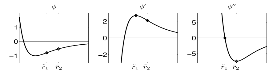
Figure 2. The Lennard-Jones potential (3.7) demonstrates the prototypical behavior of $\phi(r)$ and its derivatives.

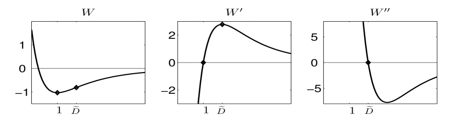
Figure 3. The energy density, $W(D),$ corresponding to the Lennard-Jones potential (3.7) and its derivatives.

We note that ${\widetilde{D}}$ is the deformation gradient of a uniform chain at the load limit.

The following theorem gives sufficient conditions on the existence of a region $\mathbf{r}=(r_{-N},\dots,r_{N})\in\Omega=(r_{L},r_{U})^{2N+1}$ in which the iteration (3.5) is well-defined and a contraction. We see that under these conditions QCE is an efficient preconditioner for the force-based equations, giving a contraction mapping for the iteration. The idea is that these quasicontinuum approximations are quite close, so that the solution of QCE gives a good approximation to the solution of QCF.

Theorem 3.1.

For a given conjugate external force, $(\Phi_{-N},\dots,\Phi_{N})$ suppose that there exist $r_{L}$ and $r_{U}$ such that

$$\frac{\hat{r}_{2}}{2}<r_{L}<r_{U},$$ (3.8)

$$\phi^{\prime\prime}(r_{U})+21\phi^{\prime\prime}(2r_{L})>0,$$ (3.9)

$$\phi^{\prime}(r_{L})+6\phi^{\prime}(2r_{L})-4\phi^{\prime}(2r_{U}) <\Phi_{j}<\phi^{\prime}(r_{U})+6\phi^{\prime}(2r_{U})-4\phi^{\prime}(2r_{L}),$$ (3.10)

for $j=-N,\dots,N.$ Then for every $\mathbf{r}^{p}\in\Omega:=(r_{L},r_{U})^{2N+1}$ there is a unique $\mathbf{r}^{p+1}\in\Omega$ such that

$$\psi^{QCE}_{j}(\mathbf{r}^{p+1})+\psi^{G}_{j}(\mathbf{r}^{p})+\Phi_{j}=0,\qquad j=-N,\dots,N.$$ (3.11)

We also have that the induced mapping is a contraction: if $\mathbf{r}^{p}\rightarrow\mathbf{r}^{p+1}$ and $\mathbf{s}^{p}\rightarrow\mathbf{s}^{p+1},$ then

$$\left|\left|\mathbf{r}^{p+1}-\mathbf{s}^{p+1}\right|\right|_{\infty}\leq\frac{16|\phi^{\prime\prime}(2r_{L})|}{\phi^{\prime\prime}(r_{U})-5|\phi^{\prime\prime}(2r_{L})|}\left|\left|\mathbf{r}^{p}-\mathbf{s}^{p}\right|\right|_{\infty},$$

where we have from (3.9) that

$$\frac{16|\phi^{\prime\prime}(2r_{L})|}{\phi^{\prime\prime}(r_{U})-5|\phi^{\prime\prime}(2r_{L})|}<1.$$

We start by remarking on the theorem’s assumptions. The second inequality in (3.8) states that $r_{L}$ is acting as a lower bound on $\min_{j}r_{j}$ and $r_{U}$ as an upper bound. The first inequality is chosen for convenience so that $\phi^{\prime\prime}(2r)$ is monotone. (We note that for Lennard-Jones and similar potentials, it is physically a very reasonable assumption due to the stiffness of the interactions.) Condition (3.9) ensures diagonal dominance of the Jacobian matrix for $F^{QCE}$ and ensures that the contraction estimate is less than 1. Finally, the condition on $\Phi_{j}$ in (3.10) restricts the external forces sufficiently to allow a simple degree theory argument to prove existence of solutions.

It is possible to choose a fairly large range for $r$ when the external forces are far from the load limit of the chain. However, as $\max_{j}\Phi_{j}$ approaches the load limit, $r$ must approach the tensile limit which makes the estimates much more sensitive. This reduces the size of $(r_{L},r_{U}).$ The hypotheses of Theorem 3.1 guarantee that the iteration (3.11) converges to the QCF approximation of a stable atomistic solution.

This theorem is a modification of Theorem 5.1 in [7]. The proof there models the QCE equations as a perturbation of the fully local quasicontinuum energy, ${\mathcal{E}}^{L}.$ The proof here follows by modifying the original proof to handle the new terms that arise from removing the assumption of symmetry of $\Phi_{j}.$ These new terms can be estimated by the techniques used to estimate similar terms analyzed in [7].

4. The Deformation of a Lennard-Jones Chain under Tension

In this section, we consider the application of Theorem 3.1 to a chain modeled by the Lennard-Jones potential (3.7). The deformation of the fixed end, $\hat{y}_{M+1}(s),$ can be set arbitrarily since the dependence on $\hat{y}_{M+1}(s)$ is given by a uniform translation. To obtain a uniform tension, we model the external force for the fully atomistic chain by $\tilde{f}_{-M}=-\Phi$ and $\tilde{f}_{j}=0$ for $j=-M+1,\dots,M.$ It then follows from (3.3) that the conjugate external force for the QC approximation is given by $\Phi_{j}=\Phi$ for all $j=-N,\dots,N.$

There are uniform solutions to the QCF equations up to the load limit $\Phi_{max}=2.7810,$ that is, if $\phi^{\prime}(r)+2\phi^{\prime}(2r)=\Phi,$ then $\mathbf{\Psi}^{QCF}(r\mathbf{e})=\Phi\mathbf{e},$ where $\mathbf{e}=(1,1,\dots,1)\in\mathbb{R}^{2N+1}$ and $\mathbf{\Psi}^{QCF}(\mathbf{r}):=\left(\psi^{QCF}_{-N}(\mathbf{r}),\dots,\psi^{QCF}_{N}(\mathbf{r})\right).$ We apply an external force very close to the load limit to get an example where continuation is necessary to ensure that the preconditioned equations converge. Define the loading path $\mathbf{\Phi}(s)=2.76s\,\mathbf{e}.$ Then solutions $\mathbf{r}(s)$ to the QCF equations satisfy $\mathbf{r}(s)=r(s)\mathbf{e}$ where

$$\phi^{\prime}(r(s))+2\phi^{\prime}(2r(s))=2.76s,\qquad s\in[0,1].$$ (4.1)

For any $s\in[0,1],$ we can apply Theorem 3.1 to this example by picking $r_{L}$ and $r_{U}$ such that

$$\frac{16|\phi^{\prime\prime}(2r_{L})|}{\phi^{\prime\prime}(r_{U})-5|\phi^{\prime\prime}(2r_{L})|}=\alpha<1,$$ (4.2)

to conclude that the iterative equation using the QCE preconditioner is a contraction mapping with contraction constant $\alpha,$ provided that (3.8)-(3.10) holds. We find $r_{L}$ and $r_{U}$ symmetrically positioned about $r(s)$ by substituting $r_{L}(s)=r(s)-\delta(s)$ and $r_{U}(s)=r(s)+\delta(s)$ into (4.2) with $r(s)$ given by the solution to (4.1) to obtain

$$\phi^{\prime\prime}(r(s)+\delta(s))+(5+16/\alpha)\phi^{\prime\prime}(2(r(s)-\delta(s)))=0.$$ (4.3)

It can be checked that (3.8)-(3.10) are satisfied with $\Phi_{j}=\Phi=2.76s$ for $j=-N,\dots,N.$ Therefore, for any initial guess $\mathbf{r}^{0}\in[r(s)-\delta(s),r(s)+\delta(s)]^{2N+1},$ the iteration step (3.5) is a contraction mapping for all $n$ with contraction rate $\alpha$ and limit point $\mathbf{r}(s)=r(s)\mathbf{e}.$ Figure 4 depicts the solution $\mathbf{r}(s)$ along with four contraction intervals that correspond to $\alpha=\frac{1}{8},\frac{1}{4},\frac{1}{2},\mathrm{and}\ \frac{8}{9}.$ For every $\alpha\leq 1$ the corresponding $\delta(s)$ is decreasing. In Section 7 we consider the contraction region corresponding to $\alpha=\frac{8}{9}$ since this contraction region terminates just beyond our maximum applied load, $\delta(1.001)=0.$

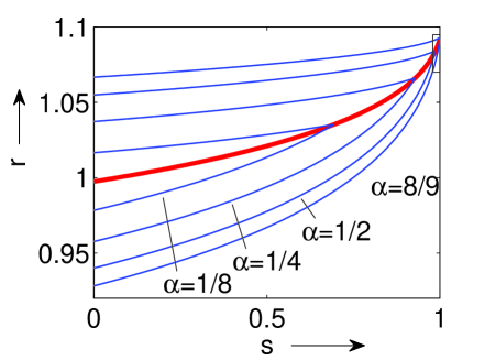
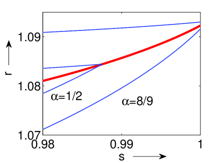
      (a)                                              (b)

Figure 4. (a) Loading response, $r(s),$ for the Lennard-Jones chain is surrounded by contraction regions, $r(s)\pm\delta(s),$ corresponding to $\alpha=\frac{1}{8},\frac{1}{4},\frac{1}{2},\frac{8}{9}$. The contraction constant $\alpha$ increases with distance from $r(s).$ (b) Detail shows the contraction region in a neighborhood of $s=1.$

4.1. Fracture at the Interface

To demonstrate the need for continuation methods for the above example, we describe the performance of a modified version of qc1d, a code by Ellad Tadmor for solving the QCF equations using QCE as a preconditioner with a nonlinear conjugate gradient method for solving the inner iteration. We attempt to directly solve (1.2) starting from the energy-minimizing lattice spacing and using only a single loading step, $Q=1,$ which gives the following minimization problem. We have

$$\mathbf{r}_{1}^{1}=\operatorname*{argmin}_{\mathbf{r}}\left[\mathbf{\Psi}^{QCE}(\mathbf{r})-\left(2.76+\mathbf{\Psi}^{G}(\mathbf{a_{0}})\right)\cdot\mathbf{R}(\mathbf{r})\right],$$ (4.4)

where $\mathbf{R}(\mathbf{r})=(\nu_{-N}r_{-N},\dots,\nu_{N}r_{N})$ denotes the representative atom spacing.

We consider an uncoarsened QC chain, with

$$M=N=7,$$

undergoing external loading as described in Section 4. The chain is partitioned with

$$K=3$$

which means that there are six atomistic representative atoms surrounded symmetrically by two groups of five continuum representative atoms. The QCF solution $\mathbf{r}(s)$ given by (4.1) and the contraction parameters $\delta(s)$ and $\alpha$ given by (4.3) do not depend on the size of the chain; however, the QCE preconditioner solution will depend on the size and composition of the chain because it has a non-uniform solution due to the atomistic to continuum interface. Because the exact solution is a uniformly deformed chain, our problem is unchanged by any coarsening of the continuum region. While this does not illustrate the power of QC approximations to reduce computational complexity, it provides a simple case in which to analyze loading up to a singular solution, in this case fracture.

The chain fractures in the atomistic to continuum interface. In the interface, QCE behaves like a continuum material with varying stiffness which is why it fails to be a consistent scheme. The corrections $\mathbf{\Psi}^{G}(\mathbf{a_{0}})$ act to counterbalance this effect by compressing the high stiffness regions, and adding tension to the low stiffness regions. Fracture occurs due to the fact that the corrections (3.6) applied in the atomistic to continuum transition are a model correction at the equilibrium bond length, $a_{0},$ but are much too strong at the stretched configuration. The overcorrections add to the very large external force and exceed the load limit for the QCE chain (see Figure 5).

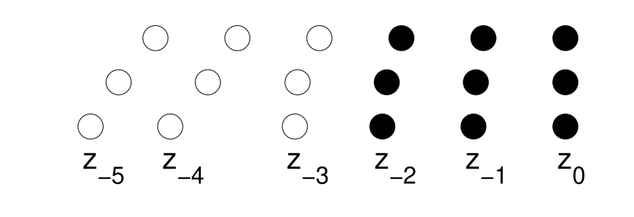
Figure 5. A close-up of the atomistic to continuum interface showing fracture that occurs when continuation is not employed. The three layers represent three steps of a single conjugate gradient minimization for the iterative equations (4.4), where the position of $z_{0}$ has been normalized to align the chains. The upper layer is the initial, undeformed state $\mathbf{r}=\mathbf{a}_{0}$. The middle layer shows a subsequent iteration where the chain is nearly uniformly deformed and close to the QCF solution. The lower layer shows later iteration where a clear separation of atom pairs occurs. None of the states shown is a solution to the minimization problem, and the numerical algorithm eventually terminates without finding a minimum.

The above estimates show that the continuation method described in Section 5 provides a convergent method for computing the deformation of the chain at the load $\Phi=2.76$ with the qc1d code.

5. Solution of the QCF Equations by Continuation

In this section and the following two, we give an analysis of the solution of the QCF equilibrium equations by continuation. We will present our results in a general setting that focuses on the contraction property of the preconditioned equations. Because we only use the abstract contraction property, the continuation analysis given here will apply to higher dimensional QC approximations provided one has a contraction result similar to Theorem 3.1. Given $G\in C^{1}(\mathbb{R}^{n+1};\mathbb{R}^{n}),$ our goal will be to approximate a curve of solutions $\mathbf{r}(s)\in C^{1}([0,1];\mathbb{R}^{n})$ to

$$G(\mathbf{r}(s),s)=0\qquad\text{ for }s\in[0,1],$$ (5.1)

where

$$\begin{split}\det\nabla_{\negthickspace\mathbf{r}}G(\mathbf{r}(s),s)\neq 0&\qquad\text{ for }s\in[0,1].\end{split}$$

We will later apply this theory to QCF by considering the solution of the equations

$$G(\mathbf{r}(s),s):=\psi^{QCF}(\mathbf{r}(s),s)+\Phi(s)=0\qquad\text{ for all }s\in[0,1].$$

Let $k(s)$ be a bound on $\mathbf{r}^{\prime}(s),$ that is, $\left|\left|\mathbf{r}^{\prime}(s)\right|\right|_{\infty}\leq k(s),$ which gives

$$\left|\left|\mathbf{r}(t)-\mathbf{r}(s)\right|\right|_{\infty}\leq\int^{t}_{s}k(\tau)\,\mathrm{d}\tau\qquad\text{for all }t>s.$$

We assume further that for each $s\in[0,1]$ there is an iterative solver $T_{s}:\mathbb{R}^{n}\rightarrow\mathbb{R}^{n}$ that is locally a contraction mapping with fixed point $\mathbf{r}(s).$ That is, there is an $\alpha<1$ such that for every $s\in[0,1],$ there is a radius $\delta(s)$ with the property

$$\left|\left|\mathbf{r}(s)-\mathbf{p}\right|\right|_{\infty},\left|\left|\mathbf{r}(s)-\mathbf{q}\right|\right|_{\infty}\leq\delta(s)\Rightarrow\left|\left|T_{s}\mathbf{p}-T_{s}\mathbf{q}\right|\right|_{\infty}\leq\alpha\left|\left|\mathbf{p}-\mathbf{q}\right|\right|_{\infty}.$$

We saw in Section 4 that such a radius $\delta(s)$ can be obtained for $T_{s}$ given by the iterative method (3.11) if the hypotheses of Theorem 3.1 are satisfied.

Let $0=s_{0}\leq s_{1}\leq\dots\leq s_{Q}=1$ be a sequence of load steps where at each point $s_{q}$ we wish to compute $\mathbf{r}_{q},$ an approximation to $\mathbf{r}(s_{q}).$ Beginning from an initial guess $\mathbf{r}^{0}_{q},$ the iterative solver $T_{s_{q}}$ is applied to (5.1), keeping $s_{q}$ fixed. This generates a sequence of approximations $\mathbf{r}^{p}_{q}=T_{s_{q}}^{p}\mathbf{r}^{0}_{q}$ for $p=1,\dots,P_{q},$ where $T_{s_{q}}^{p}$ denotes $p$ compositions of the operator $T_{s_{q}}$ and $P_{q}$ denotes the number of iterations at step $m.$ We then let $\mathbf{r}_{q}=\mathbf{r}^{P_{q}}_{q}.$ The choice of initial guess $\mathbf{r}^{0}_{q}$ is typically made using polynomial extrapolation, and here we choose $r^{0}_{q}=r_{q-1},$ which is zeroth-order extrapolation.

We will now give an analysis of how to choose the load steps $0=s_{0}\leq s_{1}\leq\dots\leq s_{Q}=1$ and the corresponding number of iterations $P_{1},\dots,P_{Q}$ to efficiently approximate $\mathbf{r}(s)$ with respect to two different goals. We first consider the efficient approximation of $\mathbf{r}(s)$ in the maximum norm for all $s\in[0,1],$ and we then consider the efficient approximation of the end point $\mathbf{r}(1).$ We note that our analysis only gives an upper bound for the amount of work needed to compute an approximation of our chosen goal to a specified tolerance since we use a uniform estimate for the rate of convergence $\alpha$ rather than the decreasing $\alpha$ as we converge to the solution that we can obtain from Theorem 3.1 and displayed in Figure 4.

6. Efficient Approximation of the Solution Path in the Maximum Norm

For simplicity, we will first consider a uniform region of contraction radius $\delta(s)=\delta,$ a uniform bound $k(s)=k,$ a uniform step size $h=1/Q=s_{q}-s_{q-1},$ and a uniform number of iterations at each step $P_{q}=P.$ We will denote the continuous, piecewise linear interpolant of $\mathbf{r}(s_{q})\in\mathbb{R}^{n},\ q=0,\dots,Q,$ by $\mathcal{I}\mathbf{r}(s);$ and we will denote the continuous, piecewise linear interpolant of $\mathbf{r}_{q}\in\mathbb{R}^{n},\ q=0,\dots,Q,$ by $\tilde{\mathbf{r}}(s).$ We will determine an efficient choice of $h$ and $P$ to guarantee that

$$\max_{s\in[0,1]}\left|\left|\mathbf{r}(s)-\tilde{\mathbf{r}}(s)\right|\right|_{\infty}\leq 2\epsilon,$$ (6.1)

where we assume for convenience that $2\epsilon\leq\delta.$

We will assume that $\mathbf{r}(s)\in C^{2}([0,1];\mathbb{R}^{n}),$ so there exists a constant $k_{2}\geq 0$ such that

$$\max_{s\in[0,1]}\left|\left|\mathbf{r}(s)-\mathcal{I}\mathbf{r}(s)\right|\right|_{\infty}\leq k_{2}h^{2}.$$

We can then ensure that

$$\max_{s\in[0,1]}\left|\left|\mathbf{r}(s)-\mathcal{I}\mathbf{r}(s)\right|\right|_{\infty}\leq\epsilon$$

by choosing $h\leq\sqrt{\epsilon/k_{2}}.$ We can thus satisfy (6.1) by guaranteeing that

$$\max_{q=0,\dots,Q}\left|\left|\mathbf{r}(s_{q})-\mathbf{r}_{q}\right|\right|_{\infty}\leq\epsilon.$$ (6.2)

Now if $\left|\left|\mathbf{r}(s_{q-1})-\mathbf{r}_{q-1}\right|\right|_{\infty}\leq\epsilon$, then

$$\left|\left|\mathbf{r}(s_{q})-\mathbf{r}^{0}_{q}\right|\right|_{\infty} \leq\left|\left|\mathbf{r}(s_{q})-\mathbf{r}(s_{q-1})\right|\right|_{\infty}+\left|\left|\mathbf{r}(s_{q-1})-\mathbf{r}_{q-1}\right|\right|_{\infty}$$

$$\leq kh+\epsilon.$$

We choose $0<h\leq\frac{\delta-\epsilon}{k}$ so that $\mathbf{r}^{0}_{q}$ is in the region of contraction

$$\left|\left|\mathbf{r}(s_{q})-\mathbf{r}^{0}_{q}\right|\right|_{\infty}\leq kh+\epsilon\leq\delta.$$

We then choose $P$ to achieve the desired error

$$\left|\left|\mathbf{r}(s_{q})-\mathbf{r}^{P}_{q}\right|\right|_{\infty} \leq\alpha^{P}\left|\left|\mathbf{r}(s_{q})-\mathbf{r}^{0}_{q}\right|\right|_{\infty}$$

$$\leq\alpha^{P}(kh+\epsilon)\leq\epsilon.$$

We can thus guarantee that $\left|\left|\mathbf{r}(s_{q})-\mathbf{r}^{P}_{q}\right|\right|_{\infty}\leq\epsilon$ by doing $P$ iterations where

$$P(h)=\frac{\ln\left(\frac{\epsilon}{\epsilon+kh}\right)}{\ln\alpha}.$$

The computational work to obtain (6.2) can then be bounded by

$${\mathcal{W}}(h)=\frac{P(h)}{h}=\frac{\ln\left(\frac{\epsilon}{\epsilon+kh}\right)}{h\ln\alpha}\quad\text{for }0\leq h\leq\frac{\delta-\epsilon}{k}.$$

We have by the Mean Value Theorem that

$$\frac{d{\mathcal{W}}(h)}{dh}=\frac{k}{h\ln\alpha}\left[\frac{\ln(\epsilon+kh)-\ln\epsilon}{kh}-\frac{1}{(\epsilon+kh)}\right]<0$$

for $0<h<\frac{\delta-\epsilon}{k}.$

We can finally obtain (6.1) by choosing

$$h_{opt} =\min\left\{\frac{\delta-\epsilon}{k},\sqrt{\epsilon/k_{2}}\right\},$$

$$P(h_{opt}) =\frac{\min\left\{\ln\frac{\epsilon}{\delta},\ln\frac{\sqrt{k}_{2}\epsilon}{\sqrt{k}_{2}\epsilon+{k}\sqrt{\epsilon}}\right\}}{\ln\alpha}\to\infty\quad\text{as}\quad\epsilon\to 0.$$

As $\epsilon$ goes to zero, the second criterion becomes active so that the step size is determined by the interpolation estimates rather than the size of the contraction region. The number of steps grows as $\frac{1}{\sqrt{\epsilon}},$ and the number of iterations per step grows like like $\frac{\ln\epsilon}{2\ln\alpha}.$

7. Efficient Approximation of the Solution at the Final State

In this section, our goal will be to compute $\mathbf{r}_{Q}$ satisfying the error tolerance

$$\left|\left|\mathbf{r}(1)-\mathbf{r}_{Q}\right|\right|_{\infty}\leq\epsilon$$ (7.1)

while minimizing the computational effort

$${\mathcal{W}}(\{P_{q}\},\{s_{q}\}):=\widehat{\mathcal{W}}\sum_{q=1}^{Q}P_{q},$$

subject to the constraints on $\{P_{q}\}$ and $\{s_{q}\}$ given below, where $\widehat{\mathcal{W}}>0$ is the work per iterative step which we scale to $\widehat{\mathcal{W}}=1.$ We note that the preceding assumes that applying the iterative solver is the most computationally expensive operation and all iterations are equally expensive. We first formulate the optimization problem with constraints, and we then simplify the problem by observing that some of the inequality constraints can be replaced by equality constraints. In this section, we now consider a continuous, decreasing contraction radius $\delta(s)$ and a continuous, positive bound $k(s).$ The load steps taken to achieve the error goal will not be uniformly spaced which will take advantage of the large initial contraction region and the fact that low error is only desired at the endpoint, $s=1.$

We define the error at $s_{q}$ by $e_{q}=\left|\left|\mathbf{r}(s_{q})-\mathbf{r}_{q}\right|\right|_{\infty}$ for all $q=0,\dots,Q.$ Then a bound on the error in the initial guess $\mathbf{r}^{0}_{q}$ for $q=1,\dots,Q$ can be given by

$$\begin{split}\left|\left|\mathbf{r}(s_{q})-\mathbf{r}^{0}_{q}\right|\right|_{\infty}&\leq\left|\left|\mathbf{r}(s_{q})-\mathbf{r}(s_{q-1})\right|\right|_{\infty}+\left|\left|\mathbf{r}(s_{q-1})-\mathbf{r}_{q-1}\right|\right|_{\infty}\\ &\leq\kappa(s_{q})-\kappa(s_{q-1})+e_{q-1},\end{split}$$

where $\kappa(s)=\int_{0}^{s}k(\tau)\,\mathrm{d}\tau.$ If $\kappa(s_{q})-\kappa(s_{q-1})+e_{q-1}\leq\delta(s_{q}),$ the mapping $T_{s_{q}}$ is a contraction and the error satisfies the bound

$$e_{q}=\left|\left|\mathbf{r}(s_{q})-\mathbf{r}^{P_{q}}_{q}\right|\right|_{\infty}\\ \leq\alpha^{P_{q}}\left|\left|\mathbf{r}(s_{q})-\mathbf{r}^{0}_{q}\right|\right|_{\infty}$$

since $\mathbf{r}(s_{q})$ is a fixed point of $T_{s_{q}}.$ We assume that $e_{0}<\delta(0),$ and we let $\{\gamma_{q}\}^{Q}_{q=0}$ be the supersolution for $\{e_{q}\}^{Q}_{q=0}$ defined by the recurrence

$$\begin{split}\gamma_{q}&=\alpha^{P_{q}}\left(\kappa(s_{q})-\kappa(s_{q-1})+\gamma_{q-1}\right),\qquad\textrm{ for }q=1,\dots,Q,\\ \gamma_{0}&=e_{0}.\end{split}$$

In the following, we satisfy the error goal (7.1) by making sure that the supersolution satisfies $\gamma_{Q}\leq\epsilon.$

We now consider the question of how to achieve the error goal for the supersolution while using the fewest possible applications of the iterative solver. We define the set of admissible loading paths that satisfy the preceding theory by

$$\begin{split}{\mathcal{A}}=\bigcup^{\infty}_{Q=1}\Big{\{}&\left(\{P_{q}\}^{Q}_{q=1},\{s_{q}\}^{Q}_{q=0}\right)\subset\mathbb{Z}^{Q-1}_{>0}\times\mathbb{Z}_{\geq 0}\times[0,1]^{Q+1}:\\ &\qquad 0=s_{0}\leq s_{1}\leq\dots\leq s_{Q}=1,\\ &\qquad\kappa(s_{q})-\kappa(s_{q-1})+\gamma_{q-1}\leq\delta(s_{q})\\ &\qquad\textrm{for all }q=1,\dots,Q,\text{ and }\gamma_{Q}\leq\epsilon\Big{\}}.\end{split}$$ (7.2)

Figure 6 shows the error $\left|\left|\mathbf{r}(s)-\hat{\mathbf{r}}(s)\right|\right|_{\infty}$ for hypothetical loading paths

$$\begin{split}\hat{\mathbf{r}}(s)=\mathbf{r}_{q-1}\quad\textrm{for }s\in[s_{q-1},s_{q}),\end{split}$$

using the worst-case error bound

$$\mathbf{r}(s_{q})-\mathbf{r}_{q}=\alpha^{P_{q}}(\mathbf{r}(s_{q})-\mathbf{r}_{q-1}).$$

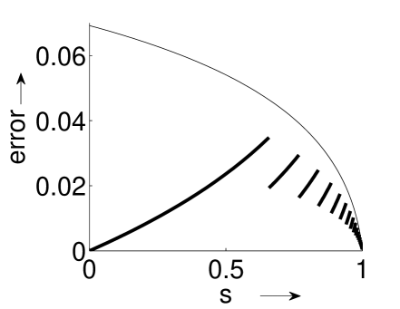
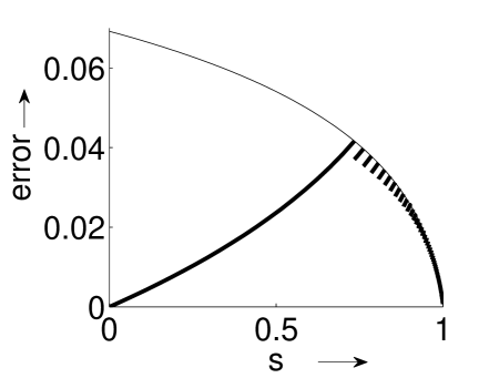
      (a)                                              (b)

Figure 6. Error $e(s)=\left|\left|\mathbf{r}(s)-\hat{\mathbf{r}}(s)\right|\right|_{\infty}$ for the deformation problem given in Section 4, where $\hat{\mathbf{r}}(s)=\mathbf{r}_{q-1},\ s\in[s_{q-1},s_{q}).$ Two example admissible loading paths (7.2) are displayed in bold. The contraction radius $\delta(s)$ corresponding to $\alpha=\frac{8}{9}$ bounds the estimated error curve for any admissible loading path. (a) Generic path with multiple iterations per step. (b) Path with a single iteration per step and error estimate just less than $\delta(s).$ Path is optimal solution for Problem 7.1.

We will next consider minimizing the work with respect to all admissible paths.

Problem 7.1.

Given $\epsilon>0,$ $\kappa(s)\geq 0$ continuous and increasing, $\delta(s)>0$ continuous and decreasing, $0\leq\gamma_{0}<\delta(0),$ and $0<\alpha<1,$ find

$$\operatorname*{argmin}_{(\{P_{q}\},\{s_{q}\})\subset{\mathcal{A}}}{\mathcal{W}}(\{P_{q}\},\{s_{q}\})=\operatorname*{argmin}_{(\{P_{q}\},\{s_{q}\})\subset{\mathcal{A}}}\ \sum_{q=1}^{Q}P_{q}.$$

We can see that ${\mathcal{A}}$ is non-empty by considering paths with sufficiently many small steps so that the error stays within the contraction domain of the iteration. Thus, the problem has a minimizer since the work for each path is a positive integer. We denote the minimum possible work by ${\mathcal{W}}_{min}.$ The above problem can be analytically solved by the using following two lemmas which characterize paths that are optimal in the sense of this problem. We first observe that it is optimal to only do enough work to stay within the contraction bounds, that is, the minimum work lies on the boundary $\kappa(s_{q})-\kappa(s_{q-1})+\gamma_{q-1}=\delta(s_{q}).$

Lemma 7.1.

Let $\mathcal{L}=(\{P_{q}\}^{Q}_{q=1},\{s_{q}\}^{Q}_{q=0})\in{\mathcal{A}}$ denote an admissible loading path. Then there is $\widehat{\mathcal{L}}=(\{\widehat{P}_{q}\}^{Q}_{q=1},\{\widehat{s}_{q}\}^{Q}_{q=0})\in A$ and $J,\,1\leq J\leq Q,$ such that $\widehat{P}_{q}=P_{q}$ for all $q=1,\dots,Q;$

$$\kappa(\widehat{s}_{q})-\kappa(\widehat{s}_{q-1})+\widehat{\gamma}_{q-1}=\delta(\widehat{s}_{q})$$ (7.3)

for every $q=1,\dots,J-1;$ and $\widehat{s}_{q}=1$ for every $q>J.$ Furthermore, $\widehat{\gamma}_{Q}\leq\gamma_{Q}$ with equality if and only if $\mathcal{L}=\widehat{\mathcal{L}}.$

The full proof is given in the Appendix. The idea is that since our goal is to only get accuracy at $s_{Q}$ (7.1), reducing error early results in extra total work. If (7.3) is not satisfied at some $s_{q},$ then we can take a larger step between $s_{q-1}$ and $s_{q}$ and smaller steps later (for $q=1,\dots,Q-1$) which reduces the supersolution for the error for all subsequent steps.

Next, we denote the set of all admissible loading paths with work $\sum^{Q}_{q=1}P_{q}\leq m$ by

$${\mathcal{A}}_{m}=\Big{\{}\left(\{P_{q}\}^{Q}_{q=1},\{s_{q}\}^{Q}_{q=0}\right)\in{\mathcal{A}}:\sum^{Q}_{q=1}P_{q}\leq m\Big{\}}\quad\textrm{ for }m\geq 0.$$

If the minimum total work is denoted by ${\mathcal{W}}_{min},$ then ${\mathcal{A}}_{{\mathcal{W}}_{min}}$ is non-empty. We now show that it is optimal to only do one iteration per step, increasing the number of steps as necessary.

Lemma 7.2.

There is a path $(\{P_{q}\}^{Q}_{q=1},\{s_{q}\}^{Q}_{q=0})\in{\mathcal{A}}_{{\mathcal{W}}_{min}}$ such that $P_{q}=1$ and (7.3) hold for all $q=1,\dots,Q-1.$ This uniquely determines $Q.$ Furthermore, this path has the lowest estimated error, $\gamma_{Q},$ of all paths in ${\mathcal{A}}_{{\mathcal{W}}_{min}}.$

The full proof is given in the Appendix where it is shown that any step other than the last with $P_{q}>1$ can be split to create a new admissible path that has the same total work and a lower error.

Combining these two lemmas, we can characterize the optimal path for solving Problem 7.1 by the following algorithm, where some equations are given in implicit form:

let $\gamma_{0}=e_{0},s_{0}=0,q=0$
while $s_{q}<1$
    $q=q+1$
    $\tilde{s}_{q}=$ solve$(\kappa(\tilde{s}_{q})-\kappa(s_{q-1})+\gamma_{q-1}=\delta(\tilde{s}_{q}))$
    $s_{q}=\min(\tilde{s}_{q},1)$
    $P_{q}=1$
    $\gamma_{q}=\alpha\delta(s_{q})$
end
$P_{Q}=\left\lceil\frac{\log\epsilon-\log(\kappa(1)-\kappa(s_{Q-1})+\gamma_{Q-1})}{\log\alpha}\right\rceil$

where $\lceil x\rceil$ is the least integer not less than $x.$

Figure 6b depicts the loading curve and optimal loading path for our example, where we directly use

$$\kappa(s):=\int^{s}_{0}\left|\left|\mathbf{r}^{\prime}(\tau)\right|\right|_{\infty}\,\mathrm{d}\tau$$

in Problem 7.1. We note that the solution depicted in Figure 6b uses information about the exact solution, both in the growth estimate $\kappa$ and in the computation of contraction regions (4.3). In practice, the results will be applied using estimates to determine $\delta$ and $\kappa.$ The lemmas provide the general intuition that it is efficient to do many steps with a single iteration per step, rather than fewer steps with many iterations per step.

Appendix A Proofs of Lemma 7.1 and Lemma 7.2

We present detailed proofs of Lemma 7.1 and Lemma 7.2, which use very similar estimates to show that a given new path is computationally favorable.

Proof of Lemma 7.1. Let $J$ be the smallest integer such that $s_{J}=1.$ If $J=1,$ then we are done; otherwise we show that if (7.3) does not hold for some $q=1,\dots,J-1,$ then we can adjust $\{s_{q}\}$ to satisfy (7.3) with a strict decrease in the total error.

Let $j$ be the smallest integer such that $\kappa(s_{j})-\kappa(s_{j-1})+\gamma_{j-1}<\delta(s_{j}).$ If $j<J,$ then our step was too conservative so we define a new stepping path $\{\widetilde{s}_{q}\}_{q=0}^{Q}.$ Let $\Delta s>0$ be chosen so that $\kappa(s_{j}+\Delta s)-\kappa(s_{j-1})+\gamma_{j-1}=\delta(s_{j}).$ We let $\Delta s=\min(\Delta s,1-s_{j})$ and define $\widetilde{s}_{q}$ by

$$\widetilde{s}_{q}=\begin{cases}s_{q},&q<j,\\ s_{j}+\Delta s,&q=j,\\ \max(s_{q},s_{j}+\Delta s),&q>j.\\ \end{cases}$$

This gives a new loading path $0=\tilde{s}_{0}\leq\tilde{s}_{1}\leq\dots\leq\tilde{s}_{Q}=1.$ By construction, steps $q=1,\dots,j$ satisfy (7.3), but we must show that all subsequent steps are inside the contraction region, that is $\kappa(\tilde{s}_{q})-\kappa(\tilde{s}_{q-1})+\gamma_{q-1}\leq\delta(\tilde{s}_{q})$ for $q>j.$ If $s_{j+1}>s_{j}+\Delta s,$ we have

$$\begin{split}\widetilde{\gamma}_{j+1}&=\alpha^{P_{j+1}}[\kappa(\tilde{s}_{j+1})-\kappa(\tilde{s}_{j})+\widetilde{\gamma}_{j}]\\ &=\alpha^{P_{j+1}}[\kappa(s_{j+1})-\kappa(s_{j}+\Delta s)+\alpha^{P_{j}}\left(\kappa(s_{j}+\Delta s)-\kappa(s_{j-1})+\gamma_{j-1}\right)]\\ &=\alpha^{P_{j+1}}[\kappa(s_{j+1})-\kappa(s_{j}+\Delta s)+\alpha^{P_{j}}(\kappa(s_{j}+\Delta s)-\kappa(s_{j}))\\ &\qquad+\alpha^{P_{j}}\left(\kappa(s_{j})-\kappa(s_{j-1})+\gamma_{j-1}\right)]\\ &<\alpha^{P_{j+1}}[\kappa(s_{j+1})-\kappa(s_{j})+\gamma_{j}]\\ &=\gamma_{j+1}.\end{split}$$

The above shows that the error supersolution $\gamma_{j+1}$ is reduced and, by consideration of the terms in brackets, that the approximation is inside the contraction region at $s_{j+1}.$ A similar argument holds for the first non-degenerate step, $s_{j^{*}}>s_{j},$ in the case $s_{j}+\Delta s>s_{j+1}.$ Since the remaining path is unchanged, we have $\tilde{\gamma}_{q}<\gamma_{q}$ for all $q=j,\dots,Q.$ We continue this process until the hypotheses are satisfied. $\square$

Proof of Lemma 7.2. We choose a path in ${\mathcal{A}}_{{\mathcal{W}}_{min}}$ of the form given by Lemma 7.1. Now, if $s_{J}=1$ for $J<Q,$ we can combine step $J$ and $J+1$ by letting $\widetilde{P}_{J}=P_{J+1}+P_{J},$ thus we can consider paths where (7.3) holds for all $q=1,\dots,Q-1.$

Now, we show that if $P_{j}>1$ for some $j<Q-1,$ then the error can be reduced by adding a new load step between $s_{j}$ and $s_{j+1}.$ Suppose the path satisfies (7.3) for all $q=1,\dots,Q-1$ and $P_{j}>1$ for some $j<Q-1.$ We will consider the new path $(\{\tilde{P}_{q}\}^{Q+1}_{q=0},\{\tilde{s}_{q}\}^{Q+1}_{q=1})\in{\mathcal{A}}_{{\mathcal{W}}_{min}}$ given by

$$\begin{split}\widetilde{P}_{q}&=\begin{cases}P_{q}&q<j\\ 1&q=j\\ P_{j}-1&q=j+1\\ P_{q-1}&q>j+1\end{cases}\\ \tilde{s}_{q}&=\begin{cases}s_{q}&q<j+1\\ s_{j}+\Delta s&q=j+1\\ s_{q-1}&q>j+1,\end{cases}\end{split}$$

where $\Delta s$ is chosen such that

$$\begin{split}\kappa(\tilde{s}_{j+1})&-\kappa(\tilde{s}_{j})+\tilde{\gamma}_{j}\\ &=\kappa(s_{j}+\Delta s)-\kappa(s_{j})+\alpha\delta(s_{j})\\ &=\delta(s_{j}+\Delta s)\\ &=\delta(\tilde{s}_{j+1}).\end{split}$$

The above has a solution, with $0<\Delta s<s_{j+1}-s_{j},$ by the Intermediate Value Theorem. The above path clearly has the same total work as the original, and we now show that it satisfies the contraction region constraints in Problem 7.1. We find that

$$\begin{split}\kappa(\tilde{s}_{j+2})&-\kappa(\tilde{s}_{j+1})+\tilde{\gamma}_{j+1}\\ &=\kappa(\tilde{s}_{j+2})-\kappa(\tilde{s}_{j+1})+\alpha^{\widetilde{P}_{j+1}}\delta(\tilde{s}_{j+1})\\ &=\kappa(s_{j+1})-\kappa(s_{j}+\Delta s)\\ &\qquad+\alpha^{P_{j}-1}\left(\kappa(s_{j}+\Delta s)-\kappa(s_{j})+\alpha\delta(s_{j})\right)\\ &<\delta(s_{j+1}).\end{split}$$

Thus, we have lowered the supersolution for the error. We can apply Lemma 7.1 and the above argument until the hypotheses are satisfied, and at each step the error supersolution is reduced. $\square$

References

- [1] M. Arndt and M. Luskin. Goal-oriented atomistic-continuum adaptivity for the quasicontinuum approximation. International Journal for Multiscale Computational Engineering, 5:407–415, 2007.
- [2] M. Arndt and M. Luskin. Error estimation and atomistic-continuum adaptivity for the quasicontinuum approximation of a frenkel-kontorova model. SIAM J. Multiscale Modeling & Simulation, 7:147–170, 2008.
- [3] M. Arndt and M. Luskin. Goal-oriented adaptive mesh refinement for the quasicontinuum approximation of a Frenkel-Kontorova model. Computer Methods in Applied Mechanics and Engineering, to appear.
- [4] R. E. Bank and D. J. Rose. Analysis of a multilevel iterative method for nonlinear finite element equations. Math. Comp., 39(160):453–465, 1982.
- [5] X. Blanc, C. Le Bris, and F. Legoll. Analysis of a prototypical multiscale method coupling atomistic and continuum mechanics. M2AN Math. Model. Numer. Anal., 39(4):797–826, 2005.
- [6] W. Curtin and R. Miller. Atomistic/continuum coupling in computational materials science. Modell. Simul. Mater. Sci. Eng., 11(3):R33–R68, 2003.
- [7] M. Dobson and M. Luskin. Analysis of a force-based quasicontinuum method. M2AN Math. Model. Numer. Anal., 42:113–139, 2008.
- [8] E. Doedel. Lecture notes on numerical analysis of bifucation problems. Electronic Source: http://cmvl.cs.concordia.ca/publications.html, March 1997.
- [9] W. E., J. Lu, and J. Yang. Uniform accuracy of the quasicontinuum method. Phys. Rev. B, 74:214115, 2006.
- [10] W. E and P. Ming. Analysis of the local quasicontinuum method. In Frontiers and Prospects of Contemporary Applied Mathematics, pages 18–32. Higher Education Press, World Scientific, 2005.
- [11] W. E and P. Ming. Cauchy-born rule and the stabilitiy of crystalline solids: Static problems. Arch. Ration. Mech. Anal., 183:241–297, 2007.
- [12] H. B. Keller. Numerical solution of bifurcation and nonlinear eigenvalue problems. In Applications of bifurcation theory (Proc. Advanced Sem., Univ. Wisconsin, Madison, Wis., 1976), pages 359–384. Publ. Math. Res. Center, No. 38. Academic Press, New York, 1977.
- [13] J. Knap and M. Ortiz. An analysis of the quasicontinuum method. J. Mech. Phys. Solids, 49:1899–1923, 2001.
- [14] P. Lin. Theoretical and numerical analysis for the quasi-continuum approximation of a material particle model. Math. Comp., 72(242):657–675 (electronic), 2003.
- [15] P. Lin. Convergence analysis of a quasi-continuum approximation for a two-dimensional material. SIAM J. Numer. Anal., 45(1):313–332, 2007.
- [16] R. Miller, L. Shilkrot, and W. Curtin. A coupled atomistic and discrete dislocation plasticity simulation of nano-indentation into single crystal thin films. Acta Mater., 52(2):271–284, 2003.
- [17] R. Miller and E. Tadmor. The QC code. http://www.qcmethod.com/.
- [18] R. Miller and E. Tadmor. The quasicontinuum method: Overview, applications and current directions. J. Comput. Aided Mater. Des., 9(3):203–239, 2002.
- [19] J. T. Oden, S. Prudhomme, A. Romkes, and P. Bauman. Multi-scale modeling of physical phenomena: Adaptive control of models. SIAM Journal on Scientific Computing, 28(6):2359–2389, 2006.
- [20] C. Ortner and E. Süli. A-posteriori analysis and adaptive algorithms for the quasicontinuum method in one dimension. Research Report NA-06/13, Oxford University Computing Laboratory, 2006.
- [21] C. Ortner and E. Süli. Analysis of a quasicontinuum method in one dimension. M2AN, 42:57–91, 2008.
- [22] S. Prudhomme, P. T. Bauman, and J. T. Oden. Error control for molecular statics problems. International Journal for Multiscale Computational Engineering, 4(5-6):647–662, 2006.
- [23] D. Rodney and R. Phillips. Structure and strength of dislocation junctions: An atomic level analysis. Phys. Rev. Lett., 82(8):1704–1707, Feb 1999.
- [24] T. Shimokawa, J. Mortensen, J. Schiotz, and K. Jacobsen. Matching conditions in the quasicontinuum method: Removal of the error introduced at the interface between the coarse-grained and fully atomistic regions. Phys. Rev. B, 69(21):214104, 2004.
- [25] E. Tadmor, M. Ortiz, and R. Phillips. Quasicontinuum analysis of defects in solids. Phil. Mag. A, 73(6):1529–1563, 1996.