PIERNIK MHD code — a multi–fluid, non–ideal
extension of the relaxing–TVD scheme (III)

Abstract

We present a new multi–fluid, grid MHD code PIERNIK, which is based on the Relaxing TVD scheme [Jin and Xin, 1995]. The original scheme (see Trac & Pen [Trac and Pen, 2003] and Pen et al. [Pen et al., 2003]) has been extended by an addition of dynamically independent, but interacting fluids: dust and a diffusive cosmic ray gas, described within the fluid approximation, with an option to add other fluids in an easy way. The code has been equipped with shearing–box boundary conditions, and a selfgravity module, Ohmic resistivity module, as well as other facilities which are useful in astrophysical fluid–dynamical simulations. The code is parallelized by means of the MPI library. In this paper we present Ohmic resistivity extension of the original Relaxing TVD MHD scheme, and show examples of magnetic reconnection in cases of uniform and current–dependent resistivity prescriptions.

1 Resistive MHD equations

Piernik MHD code is capable of dealing with resistive MHD equations [Pawłaszek, 2008], which involve the resistive dissipation term in the induction equation

$$\partial_{t}\mathbf{B}=\nabla\times\left(\mathbf{v}\times\mathbf{B}\right)-\nabla\times(\eta\mathbf{J}),$$ (1)

where $\mathbf{J}$ is the electric current density. Due to the conservative nature of the basic MHD algorithm, any decrement of magnetic energy during the update of magnetic field results in a corresponding increment of thermal energy. Therefore, no additional source term related to resistivity is needed in the energy equation.

The resistivity algorithm of PIERNIK code relies on additional terms of resistive origin in the electromotive force, supplemented to the original Constraint Transport (CT) scheme implemented by Pen et al. [Pen et al., 2003] within the Relaxing TVD scheme. In the present version of PIERNIK we have implemented a current–dependent resistivity, according to Ugai [Ugai, 1992]

$$\eta=\eta_{1}+\eta_{2}(J^{2}-J^{2}_{\textrm{\scriptsize crit}})\Theta(|\mathbf{J}|-|\mathbf{J}_{\textrm{\scriptsize crit}}|),$$ (2)

where $\eta_{1}$ is a constant corresponding to uniform resistivity, $\eta_{2}$ represents the anomalous resistivity, which switches on when the current density exceeds a certain critical value $J_{\textrm{\scriptsize crit}}$, and $\Theta$ is the Heaviside step function.

2 Resistivity algorithm

The relation between electric currents and magnetic fields in magnetized media is given by Ampere’s law

$$\mathbf{J}=\nabla\times\mathbf{B},$$ (3)

where the code normalization of current densities is applied, to get rid of the factor $c/4\pi$ in Ampere’s law. To solve the Ampere’s equation numerically in a grid scheme we set the location of current components at the cell edges, while the current–dependent resistivity values are initially placed at the cell corners (see Fig. 1 for details).

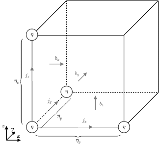
Figure 1: Position of the magnetic field $\mathbf{B}$ components, the electric current $\mathbf{J}$ components and the magnetic resistivity $\eta$ on a computational cell. Braces indicate interpolation of $\eta$ to the position of electric current density $\mathbf{J}$

To improve the stability of the resistive part of the MHD scheme a weighted average of resistivity among the closest neighbours is computed before resistive terms are taken into account in the computation of electromotive forces. Resistivity derived in this fashion is then interpolated to the positions of the current density components (cell edges) (see Fig. 1) and then the resistive part of the electromotive force $({\cal E}_{\eta}=\eta\mathbf{J})$ is computed. Eventually, we compute the diffusive terms of induction equation (1) and update magnetic field components.

3 Current sheet test

The following 2D tearing instability setup has been proposed by Hawley & Stone [Hawley and Stone, 1995] (see also the web–page of ATHENA code [Stone et al., 2008]) to test robustness of MHD algorithms at extreme conditions. The initial setup assumes magnetic field $B_{y}=\pm 1$, which changes sign at two locations $(x=\pm 0.25)$, in a domain $-0.5\leq x\leq 0.5$ and $-0.5\leq y\leq 0.5$ with doubly periodic boundary conditions. Initial density and pressure are uniform: $\rho=1$, $p=\beta/2$, where $\beta=0.1$ is the ’plasma–$\beta$’. The initial sinusoidal velocity perturbation is perpendicular to magnetic field. The initial setup consists of two current sheets at $x=\pm 0.25$, which promote magnetic reconnection, due to the numerical or physical resistivity.

We shall use the above setup to demonstrate qualitative differences between simulations with the uniform and current–dependent resistivity prescriptions. For the uniform resistivity test we assume $\eta_{1}=10^{-4}$ and $\eta_{2}=0$. It is apparent that current sheets form elongated structures, that look rather smooth, since the uniform resistivity acts everywhere in the computational domain. The uniform resistivity prescription applied in this experiment (Fig. 2), leads to configurations resembling the Sweet–Parker model (Parker [Parker, 1957]; Sweet [Sweet, 1958]).

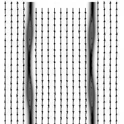
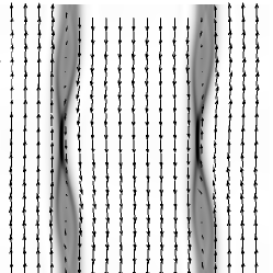
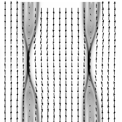
Figure 2: Snapshots of tearing instability at $t=2,4,6$ with an uniform resistivity. Grayscale represents current density and arrows denote normalized magnetic field. Resolution $512^{2}$

To simulate magnetic reconnection with anomalous resistivity we assume $\eta_{1}=0$, $\eta_{2}=10^{-4}$ and $J_{\textrm{\scriptsize crit}}=100$. The results of a 2D simulation of the tearing instability, with the initial condition specified at the beginning of this section are shown in Fig. 3. We find that in the case of localized resistivity multiple magnetic islands are formed along each current sheet, and the reconnection process is apparently more localized than in the uniform resistivity case. During the evolution smaller islands undergo coalescence to form bigger ones. Finally, two large magnetic islands remain and the reconnection tends to form small–size current sheets, resembling ’X–type’ reconnection points of Petschek’s reconnection model [Petschek, 1964]. The reconnection process is faster in the case of localized resistivity, since the final volume of magnetic islands is apparently larger than in the uniform resistivity case. Although magnetic reconnection can be observed in ’ideal MHD’ simulations due to numerical resistivity, utilization of the resistivity module allows for controlling the speed and properties of the reconnection process in MHD simulations.

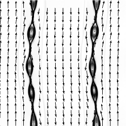
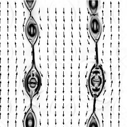
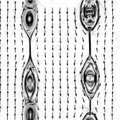
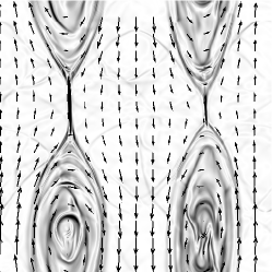
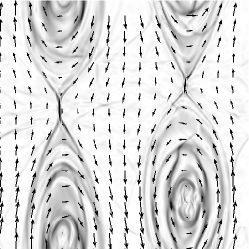
Figure 3: Snapshots of tearing instability at $t=0.8,1.2,1.6,2,4,6$ with anomalous resistivity. Grayscale, vectors and resolution as in Fig. 2.

References

- Hawley and Stone, 1995 Hawley, J. F. and Stone, J. M.: 1995, Computer Physics Communications 89, 127
- Jin and Xin, 1995 Jin, S. and Xin, Z.: 1995, Comm. Pure Appl. Math. 48, 235
- Parker, 1957 Parker, E. N.: 1957, J. Geophys. Res. 62, 509
- Pawłaszek, 2008 Pawłaszek, R.: 2008, Magnetic Reconnection in Astrophysical Disks, MSc thesis, Nicolaus Copernicus University, Toruń.
- Pen et al., 2003 Pen, U.-L., Arras, P., and Wong, S.: 2003, Astrophys. J., Suppl. Ser. 149, 447
- Petschek, 1964 Petschek, H. E.: 1964, in W. N. Hess (ed.), The Physics of Solar Flares, pp 425–+
- Stone et al., 2008 Stone, J. M., Gardiner, T. A., Teuben, P., Hawley, J. F., and Simon, J. B.: 2008, Astrophys. J., Suppl. Ser. 178, 137
- Sweet, 1958 Sweet, P. A.: 1958, in B. Lehnert (ed.), Electromagnetic Phenomena in Cosmical Physics, Vol. 6 of IAU Symposium, pp 123–+
- Trac and Pen, 2003 Trac, H. and Pen, U.-L.: 2003, Publ. Astron. Soc. Pac. 115, 303
- Ugai, 1992 Ugai, M.: 1992, Phys. Fluids, B 4, 2953