Bose-Einstein condensation of 2D dipolar excitons: Quantum Monte Carlo simulation

Abstract

The Bose condensation of 2D dipolar excitons in quantum wells is numerically studied by the diffusion Monte Carlo simulation method. The correlation, microscopic, thermodynamic, and spectral characteristics are calculated. It is shown that, in structures of coupled quantum wells, in which low-temperature features of exciton luminescence have presently been observed, dipolar excitons form a strongly correlated system. Their Bose condensation can experimentally be achieved much easily than for ideal or weakly correlated excitons.

I Introduction

Two-dimensional (2D) dipolar excitons, in which electrons ($e$) and holes ($h$) are spatially separated, can be created in structures of coupled (CQWs) quantum wells (QWs) LY and single QW (SQW) in a strong external transverse electric field js035197 . At low temperatures, $e$ and $h$ in these systems reside in the lowest transverse (with respect to the QW plane) quantized states. In this case, the dipole moments of excitons (in the ground axially symmetric state) are all directed perpendicular to this plane. There are two types of excitons in CQWs: direct excitons, whose electrons and holes are in the same QW, and spatially indirect excitons, whose electrons and holes are located in different QWs (see details in experimental studies revM ; revS ; revT ; revB ; T ; B ; M ; Snoke1 ; ss134037 ; rl970103 ; b7400409 ; transp ). In the second case, exciton dipole moment is $d=eD$, where the quantity $D$ is determined by the geometry and is equal to the characteristic interwell distance (see Eq. (3) below). In single quantum wells, a dipolar exciton can occur due to a strong transverse electric field, which induces a dipole moment js035197 ; TSQW . In both cases, unlike quasi-2D atomic gases rl842551 , two 2D dipolar excitons cannot pass ”over one another” in the QW plane. Dipolar interaction of 2D excitons is theoretically studied in Ref. 2DDE .

At low exciton densities, 2D dipolar excitons are far from each other, so exchange effects between electrons (holes) of neighboring excitons are suppressed by a dipole barrier, related to a exciton dipole-dipole repulsion,

$$P\sim\exp\left(-\int_{a_{ex}}^{a_{cl}}\sqrt{m(V(r)-2E_{0}/N)}dr\right).$$

Here, $P$ is the probability for a 2D dipolar exciton to tunnel through the dipole barrier; $m$ is the exciton mass; $E_{0}$ is the ground-state energy of the excitons (their kinetic and dipolar-interaction energies); $N$ is the exciton number; $V(r$) is the dipolar exciton potential; $a_{ex}$ is the exciton diameter (which is of the order of the average distance $a_{eh}$ between $e$ and $h$ in the exciton); and $a_{cl}$ is the classical turning point for the potential $V(r)$ ($V(a_{cl})=2E_{0}/N$). In this case, 2D dipolar excitons can be considered as (composite) bosons. At high exciton densities, at which the distance between neighboring excitons is smaller or of the order of the exciton radius, the Fermi properties of the internal exciton structure play a significant role. This leads to a transformation of a dipolar exciton gas into an $e$-$h$ system LB0 ; prl100256402 (although, in the isotropic system at $T=0$, the crossover from an exciton Bose condensate to a BCS state, with the gap decreasing with an increase in the density, occurs LY ).

The possibility of the Bose condensation of 3D excitons was under consideration long ago KK . However, in a homogeneous infinite 2D system, because of the ultraviolet divergence of the exciton momentum distribution, the Bose condensation is possible only at $T=0$ r1580383 . In the range of finite temperatures, only a quasi-long-range (power-law) order PFCT and a superfluid phase can occur, which are destroyed due to the dissociation of pairs of oppositely directed vortices and formation of free vortices at the Berezinskii-Kosterlitz-Thouless (BKT) transition point Berezinskii ; jc061181 ; jc071046 ; rl391201 . However, in finite 2D systems (traps), the ultraviolet divergence of the momentum distribution is cut off, so, the Bose condensate can exist rl842551 ; 2DBEC . This opens opportunities for studying the Bose condensation of 2D dipolar excitons in real experimental systems.

At present, the search for the Bose condensation of 2D dipolar excitons in CQWs revM ; revS ; revT ; revB and in SQW has attracted much attention from researchers. Interesting optical effects observed in studying the luminescence of 2D dipolar excitons in CQWs at low temperatures point to significant experimental progress in the investigation of the collective properties of 2D dipolar excitons T ; B ; M ; Snoke1 ; ss134037 ; rl970103 ; b7400409 ; transp . The observations of a narrow-beam luminescence from a 2D dipolar exciton Bose condensate along a normal to the QW plane and of the off-diagonal long-range order of Bose condensed 2D dipolar excitons in the coherence experiment have recently been performed by Timofeev et al. in SQW in a transverse electric field TSQW .

Theoretically, for the collective state of 2D dipolar excitons in QWs, superfluidity SF ; SFB ; LB , Bose condensation LB0 ; LB ; BEC (in the exciton regime), a BCS-like state LY ; BCS (in the $e$-$h$ system), strong correlations js035197 ; MCLKAW , crystallization js035197 ; cr ; MCcr ; rl980605 ; MCcrLKAW and a mesoscopic supersolid phase SS , kinetic and relaxation processes kinrel , vortical V and quasi-Josephson QD effects, optical properties opt as well as these in circular traps ring , a superfluid transition (crossover) in traps LKW , as well as the effect of random fields SFB ; rand , were studied.

The superfluidity of Bose condensed dipolar excitons was also studied in two-layer $e$-$e$ systems in a strong magnetic field with the half-occupancy of the Landau levels in each layer ($\nu=1/2+1/2$; see, e.g., the theory in Ref. 2DEEt and experiments in Ref. 2DEEe and references therein).

2D dipolar bosons were also studied in rarefied atomic gases dipat and polar molecules polmol .

Among the above studies into the exciton Bose condensate, the model of an ideal exciton gas and that of a weakly correlated exciton gas were predominantly used as theoretical approaches. Unfortunately, these approaches have a rather limited domain of applicability. Indeed, at low densities, the repulsive dipole potential can be described by only one parameter, the length $a_{s}$ of the isotropic $s$-scattering. Therefore, the properties of such a potential should be universal, i.e., the same for all interaction potentials having the same scattering length; in particular, the properties should be the same as for the system of hard disks with the diameter $a_{s}$. However, the latter system is known to be weakly correlated only in the ultrararefied case HD . Consequently, the model of weakly correlated excitons is valid only for ultrararefied systems, whose critical temperature is extremely low. For real experimentally observed densities, this model can give only a qualitative description. Therefore, the quantitative theoretical investigation of the 2D QW dipolar exciton collective state requires a more accurate model and more precise, desirably, ab initio, calculations.

This work is devoted to the detailed microscopic investigation of 2D dipolar excitons by means of the numerical simulation by the diffusion Monte Carlo method. The main result of our simulation is the inference that, in the experimentally observed low-temperature regime revT ; revB ; T ; B ; M , 2D dipolar excitons in CQWs form a strongly correlated system Butovring . We find the following evidences for this fact.

(i) The dimensionless adiabatic compressibility $\zeta=m^{3}/$ $\!\!(2\pi\hbar^{2}\chi)$ ($\chi$ is the corresponding dimensional quantity) and the contribution $\zeta^{\prime}=\mu_{i}m/(2\pi\hbar^{2}n)$ to the chemical potential $\mu_{i}$ related to the dipolar exciton-exciton interaction prove to be much greater than unity, $\zeta,\zeta^{\prime}\gg 1$ (Here, $n$ is the total exciton density in all the $g_{ex}$ spin degrees; $g_{ex}=4$ for GaAs). For weakly correlated excitons, $\zeta,\zeta^{\prime}\ll 1$.

(ii) The density $n_{0}$ of the exciton Bose condensate (in all the $g_{ex}$ spin degrees) at $T=0$ proves to be two to four times smaller than the total density $n$ (in the regime of weak correlations, $n_{0}\approx n$).

(iii) A clearly pronounced hump is observed both in the pair distribution function and in the structure factor, which points to the presence of the short-range order. In addition, at higher exciton densities, e.g., at $n=5\cdot 10^{10}$ cm^-2, two humps are observed in the structure factor and three in the pair distribution function.

(iv) The spectrum of excitons is very far from the Bogolyubov shape (although, even at the boundary between the exciton and $e$-$h$ regimes, the roton minimum is not yet reached under the experimental conditions of Refs. revT ; revB ; T ; B ; M ).

(v) The local superfluid exciton density at the superfluid transition temperature, $n_{l}(T_{c})$, is close to the total exciton density $n$ (whereas, for weakly correlated systems, the quantity $n_{l}(T_{c})$ is logarithmically small compared to $n$ b3704936 ) nl=n .

(vi) The temperature of the superfluid transition in the corresponding infinite system is only slightly less than the degeneracy temperature $T_{deg}$, while the quasi-condensation temperature is 2-2.5 times higher than $T_{deg}$ (for the spin-depolarized exciton gas in all the $g_{ex}=4$ spin degrees). In contrast, according to the theory of weakly correlated excitons, these temperatures are logarithmically small compared to $T_{deg}$ b3704936 .

(vii) The profile of the exciton Bose condensate in a large 2D harmonic trap at $T=0$ appreciably differs from the Thomas-Fermi inverted parabola.

In some structures of CQWs Snoke1 ; ss134037 and SQW TSQW , the condensed gas of 2D dipolar excitons forms a system with intermediate correlations ($\zeta,\zeta^{\prime}\sim 1$). In this case, the above evidences weaken (evidence (iii) vanishes). However, in structures of CQWs and SQW with the width of these wells being sufficiently large, at high densities of excitons, their correlations prove to be so strong that a roton minimum appears (and even the crystallization of excitons is possible; see, e.g., Refs. rl980605 ; MCcrLKAW ).

The paper is organized as follows. In Section II, the model is discussed, the problem is formulated, and the relation with experiment is considered. Also, the details of simulation are presented. Section III is devoted to a homogeneous exciton system. A detailed analytical processing is constructed based on the ab initio numerical simulation, with the microscopic parameters of the problem being calculated. Using these results, in Section IV, we analytically investigate a large harmonic trap in the local density approximation. The possibilities of experimental observation of strong correlations in the system of 2D dipolar excitons in CQWs are discussed in Section V. In section VI we conclude the study.

II Model and calculation method

Two 2D spatially separated excitons repel each other as dipoles, $V(r)\propto 1/r^{3}$, if the distance between them is much longer than the effective spacing $D$ between $e$ and $h$ layers. In the exciton regime, the distance between neighboring excitons in structures of Refs. revT ; revB ; T ; B ; M ; Snoke1 ; ss134037 ; rl970103 ; b7400409 ; transp ; TSQW , according to a rough estimate (see details in b3206601 ), exceeds $D$. Therefore, the model of dipolar excitons is a good approximation for experimentally studied systems. The suppression of the exchange interaction by the dipole barrier in the exciton regime makes it possible to consider 2D dipolar excitons as structureless bosons LB0 .

As a result, at $r\gg D$, we arrive at the following Hamiltonian of the homogeneous system of structureless 2D dipolar excitons:

$$\hat{H}=\frac{\hbar^{2}}{mx_{0}^{2}}\left(\sum_{i}\frac{\bar{\Delta}_{i}}{2}+\sum_{i<j}\frac{1}{\bar{r}_{ij}^{3}}\right).$$ (1)

Here,

$$x_{0}=\frac{md^{2}}{4\pi\varepsilon\varepsilon_{0}\hbar^{2}}=\frac{me^{2}D^{2}}{\varepsilon\hbar^{2}}>0$$ (2)

is the parameter with the dimension of length for the exciton dipole-dipole potential $V(r)$,

$$V(r)=\frac{\hbar^{2}}{m}\frac{x_{0}}{r^{3}},\;\;\;\;\bar{r}_{ij}=\frac{|{\bf r}_{i}-{\bf r}_{j}|}{x_{0}},$$

$$\bar{\Delta}_{i}=x_{0}^{2}\Delta_{i},\;\;\;\;\Delta_{i}=\partial^{2}/\partial x_{i}^{2}+\partial^{2}/\partial y_{i}^{2}+\partial^{2}/\partial z_{i}^{2},$$

$d=eD$ is the dipole moment of an exciton, $e>0$ is the hole charge, $\varepsilon$ is the dielectric constant of the structure, $\varepsilon_{0}=1/4\pi$ is the dielectric permittivity of vacuum, and

$$D=\left|\int_{-\infty}^{\infty}(|\psi_{e}(z)|^{2}-|\psi_{h}(z)|^{2})zdz\right|$$ (3)

is the effective distance between the $e$ and $h$ layers, where $\psi_{e}(z)$ and $\psi_{h}(z)$ are, respectively, the electron and the hole wave functions along the $z$ axis.

We impose periodic boundary conditions. This, on the one hand, makes the system finite and, on the other hand, imitates its homogeneity. In this case, the momentum becomes discrete but remains good quantum number.

At the first stage, in calculations by the variational Monte Carlo method, we specify the trial function of the ground state of excitons to be a Bijl-Jastrow function

$$\psi_{T}({\bf r}_{1}...{\bf r}_{N})=\prod_{i<j}f(\bar{r}_{ij}),$$ (4)

where,

$$f(\bar{r})=\left\{\begin{array}[]{ll}AK_{0}(2/\sqrt{\bar{r}}),&\bar{r}<\bar{r}_{c},\\ B\exp(-C/\bar{r}-C/(\bar{L}-\bar{r})),&\bar{r}_{c}\leq\bar{r}<\bar{L}/2.\end{array}\right.$$ (5)

Here, $K_{0}(x)$ is the modified Bessel function of the second kind (the Macdonald function) of the zeroth order, $\bar{r}=r/x_{0}$, and $\bar{L}=L/x_{0}$ is the dimensionless size of the system $L$. The constants $A$, $B$, and $C$ are chosen from the condition $f(\bar{L}/2)=1$ and continuity conditions of the zeroth and first derivatives at $\bar{r}=\bar{r}_{c}$, and the joining point $\bar{r}_{c}$ is used as the (only) variational parameter. We expect that the trial wave function (4) is a good approximation for the wave function of the ground state. When two excitons approach close each other, the influence of remaining exciton pairs becomes small, and the function $f(\bar{r})$ corrresponds to the solution of the two-particle scattering problem from the dipole-dipole potential. At short distances, function (5) is chosen such that it corresponds to the exact solution of the scattering problem for zero energy. We also verified that the use of the numerical solution to the scattering problem at finite energy as a two-particle factor of $f(\bar{r})$ in the Bijl-Jastrow function weakly varies the variational energy of the system and almost does not affect the diffusion value of the energy. The long-wavelength behavior of the function $f(\bar{r})$ is determined by the collective properties and corresponds to the phonon propagation in the 2D system: $f(\bar{r})\propto e^{-const/\bar{r}}$ r1550088 . The second term is added to the exponent of the exponential in Eq. (5) in order to satisfy the condition that the derivative at the boundary of the box is zero: $f^{\prime}(L/2)=0$. The function $f(\bar{r})$ is shown in Fig. 1.

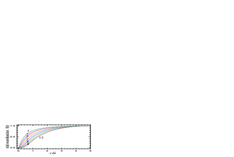
Figure 1: Trial wave function $f(r)$ at different exciton densities $n$. Curve $i$ ($i=1,2...12$) corresponds to the density $nx_{0}^{2}=2^{i-9}$. Circles show the point $r_{c}$ of joining of two asymptotics.

As is seen from Eqs. (1), (4), and (5) the Hamiltonian and the trial function are reduced to the dimensionless forms that are expressed, respectively, in terms of the linear units $x_{0}$ and energy units $\hbar^{2}/mx_{0}^{2}$. As a result, the dimensionless exciton density $\bar{n}=nx_{0}^{2}$ is the only dimensionless parameter of the problem.

The quantity $1/x_{0}^{2}$ yields the 2D exciton density $n$, which corresponds to the dimensionless density $\bar{n}=nx_{0}^{2}=1$ and which can be calculated by Eq. (2). Now, we will consider the range of variation of the dimensionless density $\bar{n}$ in various real experimental systems.

(1) For the structure of GaAs/AlAs CQWs studied by Timofeev and colleagues revT ; T ($D=13.6$ nm, $m=0.22m_{0}$ ($m_{0}=9.1083\cdot 10^{-28}$ g is the free electron mass), and $\varepsilon=12.5$), $1/x_{0}^{2}=2.64\cdot 10^{10}$ cm^-2.

(2) For the structure of GaAs/AlGaAs CQWs (Butov et al. revB ; B , $D=12.3$ nm, $m=0.22m_{0}$, and $\varepsilon=12.5$), $1/x_{0}^{2}=3.94\cdot 10^{10}$ cm^-2.

(3) For the structure of asymmetric GaAs/AlGaAs CQWs (Moskalenko et al. M , $D=14.1$ nm, $m=0.22m_{0}$, and $\varepsilon=12.5$), $1/x_{0}^{2}=2.28\cdot 10^{10}$ cm^-2.

(4) For the structure of InGaAs/GaAs CQWs (Snoke et al. Snoke1 ; ss134037 , $D=10.5$ nm, $m=0.14m_{0}$, and $\varepsilon=12.5$), $1/x_{0}^{2}=1.83\cdot 10^{11}$ cm^-2.

(5) For the structure of GaAs/AlGaAs CQWs (Snoke et al. rl970103 ; b7400409 , $D=15.5$ nm, $m=0.22m_{0}$, and $\varepsilon=12.5$), $1/x_{0}^{2}=1.56\cdot 10^{10}$ cm^-2.

(6) For the structure of GaAs SQW (Timofeev et al. TSQW , $D\approx 6$ nm, $m=0.22m_{0}$, and $\varepsilon=12.5$), $n=1/x_{0}^{2}\sim 7\cdot 10^{11}$ cm^-2, which corresponds to the dimensionless density $\bar{n}=1$.

Next, we have to know the range of variation of the 2D exciton density $n$ in their experimentally achievable condensed state.

The upper limit of the density is the boundary between the strong and weak coupling regimes (corresponding to the condensed exciton state and to the BCS-like $e$-$h$ state). For structure (1) revT ; T (with an average electron-hole distance of $a_{eh}=17$ nm T ), the corresponding critical density determined according to the rough estimate of Ref. b3206601 is

$$n_{max}=\frac{0.117g_{ex}}{\pi a_{eh}^{2}}\approx 5.17\cdot 10^{10}\mbox{ cm}^{-2},\;\;\;\;\bar{n}_{max}\approx 1.96$$ (6)

(here, it is taken into account that, in GaAs, excitons are in the $g_{ex}=4$ spin degrees).

Therefore, characteristic exciton densities that can be achieved in modern experiments in QWs, at which low-temperature features in exciton luminescence are observed revT ; revB ; T ; B ; M , lie in the range $10^{10}\leq n\leq 5\cdot 10^{10}$ cm^-2, i.e., $1/4\lesssim\bar{n}\lesssim 4$.

However, in very wide (wider than 100-200 nm) SQWs based on GaAs, such high dimensionless densities ($\bar{n}_{max}>290$ MCcrLKAW ) can be achieved at which excitons crystallize rl980605 .

We performed simulation in the range of the dimensionless density $1/256\leq\bar{n}\leq 8$. For structure (5) rl970103 ; b7400409 (in which the exciton correlations are stronger than in other structures), at the density $\bar{n}=8$, the dimensional exciton density is high: $n=1.2\cdot 10^{11}$ cm^-2. In structure (6) TSQW (where the exciton correlations are weaker than in other structures), at the dimensionless density $\bar{n}=1/256$ (and at the corresponding dimensional density $n\approx 2.7\cdot 10^{9}$ cm^-2), the superfluid crossover temperature of excitons in a trap of about 100 $\mu$m in size is low: 0.12 K (see LKW and Section III.6).

We should note that, in a sufficiently weak electric field, very small dipole moments $eD$ and very low dimensionless densities $\bar{n}=nx_{0}^{2}\propto D^{4}$ (see Eq. (2)) can be realized in SQWs. However, we are not interested in this case. Indeed, at $D\to 0$, the contribution of the van der Waals potential to the exciton scattering length $a_{s}$ ($a_{s}^{WDW}\sim a_{eh}$) considerably exceeds the contribution from the dipole potential to this parameter ($a_{s}^{D}=3.17222x_{0}\propto D^{2}\to 0$). As a result, excitons efficiently loose the property of dipolarity.

Nevertheless, in GaAs-based SQWs ($m=0.22m_{0}$, $\varepsilon=12.5$, $a_{eh}\approx 12$ nm), in a sufficiently weak electric field, the dimensionless density of a rarefied 2D dipolar exciton gas with a superfluid crossover temperature of about 0.1 K and with a dipole scattering length of the order of $a_{eh}$ can be rather low: $\bar{n}\sim 2^{-11}=1/2048$.

We performed the simulations by the quantum Monte Carlo (MC) method for 12 different densities $\bar{n}=2^{i-9}$ ($i=1,2...12$) in the range $1/256\leq\bar{n}\leq 8$. The number of excitons was taken to be $N=100$. Initially, we performed the calculations by the variational MC (VMC) method with the trial function defined by (4), (5) and optimized the parameter $\bar{r}_{c}$. At the second stage, the calculations were performed using the ab initio diffusion MC (DMC) method b4908920 , in which, to accelerate the convergence, the same trial function was taken but with the parameter $\bar{r}_{c}$ being already optimized.

As is known, the inaccuracy of the trial function introduces an additional error in the calculation of correlators by the DMC method. To reduce this error, the data obtained by the two variants of the MC method were linearly extrapolated, which allowed us to eliminate the first order with respect to the small difference between the exact and trial functions of the ground state b5203654 .

III Measurement results. A homogeneous system

In sections III and IV, we will use the dimensionless system of units $\hbar=m=x_{0}=1$, so, $\bar{n}=n$, $\bar{L}=L$, etc.

III.1 The the ground state energy. The chemical potential. The adiabatic compressibility

The total energy of the ground state of a two-dimensional dipolar exciton can be represented as the sum of two terms,

$$E_{tot}=\frac{2\pi Nne^{2}D}{\varepsilon}+E_{0}.$$ (7)

The first term corresponds to the energy of a capacitor formed by plane-parallel $e$ and $h$ layers spaced by the effective distance $D$. The second term is responsible for the kinetic energy of $N$ dipoles and for their dipolar interactions. It is equal to the energy of the ground state of the system of these dipoles. This energy is calculated by the DMC method.

The exciton chemical potential counted from the exciton band edge can be expressed via their total energy (7) as

$$\mu=\frac{dE_{tot}}{dN}=\mu_{e}+\mu_{i},$$ (8)

where $\mu_{e}=4\pi ne^{2}D/\varepsilon$ is the electrostatic contribution, and

$$\mu_{i}=\frac{dE_{0}}{dN}$$ (9)

is the contribution to the chemical potential of excitons, which corresponds to their interactions. This term defines the adiabatic compressibility of excitons $\chi$, $1/\chi=\int(\delta\mu_{i}/\delta n({\bf r}))d{\bf r}$. For a homogeneous system ($n({\bf r})\equiv n$), the variational derivative is reduced to the ordinary derivative ($\int(\delta\mu_{i}/\delta n({\bf r}))d{\bf r}=d\mu_{i}/dn$), so

$$1/\chi=\frac{d\mu_{i}}{dn}.$$ (10)

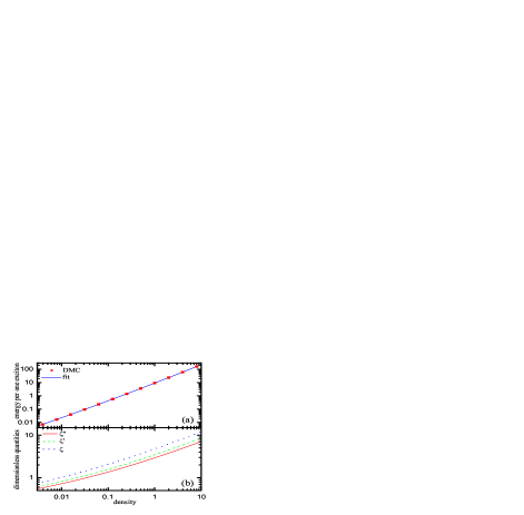
Figure 2: (a) Ground state energy per one exciton, $E_{0}/N$, as a function of the density (squares are the DMC data) and polynomial fitting curve (11) (we set $\hbar=m=x_{0}=1$). (b) Dimensionless characteristics analytically calculated from the polynomial fitting of (11) as functions of the density: energy $\zeta^{\prime\prime}$ per one exciton; contribution $\zeta^{\prime}$ to the chemical potential related to dipolar interactions; and adiabatic compressibility $\zeta$ at $T=0$.

Figure 2(a) presents the results of the DMC simulation of the ground-state energy of interacting dipoles per one particle, $E_{0}/N$, at different densities. The calculated values lie with a high accuracy (within the limits of 0.025%!) on the curve of the polynomial fitting

$$E_{0}/N=a_{e}\exp(b_{e}\ln n+c_{e}\ln^{2}n+d_{e}\ln^{3}n+e_{e}\ln^{4}n),$$ (11)

where $a_{e}=9.218$, $b_{e}=1.35999$, $c_{e}=0.011225$, $d_{e}=-0.00036$, and $e_{e}=-0.0000281$.

Figure 2b shows the energy per particle, $E_{0}/N$, the contribution to the chemical potential $\mu_{i}$ that is caused by dipolar interaction, and the adiabatic compressibility $\chi$ which were analytically calculated from the fitting to energy (11) (see Eqs. (9), (10)) and were expressed in terms of the quantities $\zeta^{\prime\prime}$, $\zeta^{\prime}$, and $\zeta$ respectively,

$$E_{0}/N=\pi n\zeta^{\prime\prime},$$ (12)

$$\mu_{i}=2\pi n\zeta^{\prime},$$ (13)

$$1/\chi=2\pi\zeta.$$ (14)

We find from this simulation that, in the entire range of calculated densities, the dimensionless adiabatic compressibility (i.e., the dimensionless interaction) proves to be greater than or of the order of unity,

$$\zeta\geq 0.774\sim 1,\;\;\;\;1/256\leq n\leq 8.$$ (15)

In the regime of high densities ($1/4\lesssim\bar{n}\lesssim 4$), we find that $\zeta\gg 1$ (see Fig. 2(b)). This testifies to strong correlations in the dense gas of 2D dipolar excitons in CQWs, whose condensation was studied in Refs. revT ; revB ; T ; B ; M .

At low densities, the quantity $\zeta\sim 1$. This is the regime of intermediate correlations, which was realized in Refs. Snoke1 ; ss134037 ; TSQW .

The regime of weak correlations ($\zeta\ll 1$) has not been realized even at the lowest calculated density $n=1/256$ (at which the superfluid crossover temperature in structures considered in Refs. revT ; revB ; T ; B ; M ; Snoke1 ; ss134037 ; rl970103 ; b7400409 ; transp ; TSQW is not higher than 0.12 K; see Section II).

III.2 The one-body density matrix. The Bose condensate fraction. The microscopic phonon length scale

On long-wavelength scales $r$ that exceed a certain value $r_{0}$ (i.e., at $r\gg r_{0}$), for the polar-circle-averaged one-body density matrix

$$\rho_{1}(r)=\int_{0}^{2\pi}\langle\hat{\Psi}^{+}({\bf r})\hat{\Psi}(0)\rangle d\varphi/2\pi$$ (16)

of Bose condensed 2D dipolar excitons, the following hydrodynamic expression holds at $T=0$ (see Appendix A):

$$\rho_{1}^{\rm hd}(r)=n_{0}\!\int\limits_{0}^{2\pi}\!\exp\!\left(\sum_{{\bf p}\neq 0}e^{i{\bf pr}}\left(\frac{\varepsilon_{p}}{2Np^{2}}-\frac{1}{4N}\!\right)\!-\frac{1}{4N}\right)\frac{d\varphi}{2\pi},$$ (17)

$$r\gg r_{0}.$$

In Eqs. (16) and (17) $\hat{\Psi}({\bf r})$ is the exciton field operator, $\langle...\rangle$ is the averaging over the exciton ground state, $\varphi$ is the polar angle of the vector ${\bf r}$, $\varepsilon_{p}$ is the excitation spectrum at $T=0$ (which we approximately determine from the structure factor by the Feynman formula; see Sections III.4, III.5), and $r_{0}$ is the characteristic microscopic phonon length scale of the system that separates the long-wavelength (hydrodynamic, $r\gg r_{0}$) and microscopic ($r\ll r_{0}$) ranges (Fig. 3(b)) and corresponds to the ultraviolet limit of applicability of the hydrodynamic method. The fact that the sum in Eq. (17) is discrete with respect to momentum (${\bf p}=(2\pi/L){\bf n}$, where ${\bf n}=\{n_{x},n_{y}\}\neq 0$ is the integer-valued vector) allows us to correctly take into account both the finiteness of the size of the system and the periodic boundary conditions.

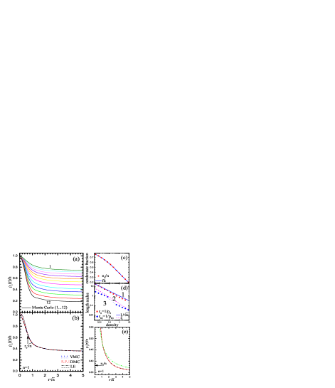
Figure 3: (a) One-body density matrix $\rho_{1}(r)$ at $T=0$ for 12 different densities ($n=2^{i-9}$, $i=1,2...12$). (b) One-body density matrix calculated by the VMC and DMC methods, as well as linear extrapolation (LE) of VMC and DMC results (thick curves) and hydrodynamic fits (thin curves) at $n=1$ (the curves practically coincide). The arrow shows the characteristic microscopic phonon length scale $r_{0}$ (in units of $1/\sqrt{n}$). (c) Bose condensate fraction at $T=0$ ($n/n_{0}$) and polynomial fitting by Eq. (19) as functions of the density. (d) Characteristic microscopic length scales of the system: phonon scale $r_{0}$, ideal-gas scale (see Section III.5) $r_{IG}$, healing length $\xi$, and interexciton distance $1/\sqrt{n}$ as functions of the density. The hydrodynamic (1), intermediate (2), and ideal-gas (3) ranges are shown. (e) One-body density matrix $\rho_{1}(r)$ at $n=1$ and large $r$: DMC calculation (dashed curve), hydrodynamic calculation (17) (solid curve), and asymptotic form (18) for the infinite system (dot-and-dash curve). The endpoint $r/\sqrt{n}=5$ of the abscissa axis corresponds to the boundary $L/2$ of the system.

The MC data for the one-body density matrix $\rho_{1}(r)$ (the linear extrapolation of the VMC and DMC data) at different exciton densities are shown in Fig. 3(a).

As shown in Fig. 3(b) the excelent coinciding of VMC and DMC results (within the line thickness) is the evidence of a good choice of the trial wavefunction and, consequently, a high accuracy of our simulation.

Figure 3(e) shows the one-body density matrix $\rho_{1}(r)$ calculated at $n=1$ and large $r$. This calculation ideally coincides (within the line thickness) with the hydrodynamic equation (17). This testifies to the internal consistency of our MC simulation, to the high measurement accuracy, and to the validity of the hydrodynamic description in this range.

For comparison, Fig. 3(e) presents the asymptotic form for the one-body density matrix at large $r$ in the corresponding infinite system ($L\to\infty$) at $n=1$,

$$\rho_{1}^{\infty}(r)=n_{0}^{\infty}\left(1+\frac{c_{s}}{4\pi n}\frac{1}{r}\right),\;\;\;\;L\to\infty,\;r\gg r_{0},1/c_{s},$$ (18)

which was obtained from Eq. (17) by the formal replacement of the sum over ${\bf p}$ by the integral. In Eq. (18), the exponential is expanded into a series, $c_{s}=\sqrt{n/\chi}$ is the sound velocity at $T=0$, and $n_{0}^{\infty}=0.3405\pm 0.001$ is the density of the Bose condensate in the infinite system at $n=1$. The quantity $n_{0}^{\infty}$ was obtained by quadratic extrapolation of the values of $\rho_{1}(L/2)$ to the macroscopic limit with respect to the powers of $1/N$ using 14 values of the total exciton number $N$ from 25 to 200.

In Fig. 3(c), the density dependence of the the exciton Bose condensate fraction is presented, which was obtained by the best fitting of hydrodynamic equation (17) to the MC data. The results are described well (within the limits of 0.005) by the following polynomial fitting curve:

$$n_{0}/n=a_{0}^{n}\exp(b_{0}^{n}\ln n+c_{0}^{n}\ln^{2}n+d_{0}^{n}\ln^{3}n),$$ (19)

where $a_{0}^{n}=0.3822$, $b_{0}^{n}=-0.2342$, $c_{0}^{n}=-0.02852$, and $d_{0}^{n}=-0.001594$. According to the data presented in Fig. 3(c), $n_{0}/n\approx 1/3$ at $n=2$, and, at $n=8$, the fraction of the Bose condensate amounts to only $n_{0}/n\approx 1/5$. This is indicative of strong correlations in the dense gas of 2D dipolar excitons in CQWs in their experimentally observed collective state. It should be specially noted that, at so small fractions of the condensate, the application of the mean-field methods (the Gross-Pitaevskii mean-field approach), the perturbation theory calculations, as well as the Bogoliubov approximation, is unjustified and can be used only for qualitative purposes.

We also note that, in the macroscopic limit ($N\to\infty$), the Bose condensate fraction is even smaller than that at $N=100$. Thus, at $n=2$ and $n=8$, respectively, we found that $n_{0}/n\approx 0.29$ and $n_{0}/n\approx 0.17$.

Figure 3(b) shows that hydrodynamic expression (17) excellently coincides with the MC calculation of $\rho_{1}(r)$ at distances $r$ longer than the characteristic microscopic phonon length scale $r_{0}$ (i.e., at $r>r_{0}$). However, at $r<r_{0}$, this coincidence vanishes very rapidly. Therefore, the crossover range of the domain of applicability of hydrodynamics for 2D dipolar excitons turns out to be very narrow.

The behavior of the characteristic linear microscopic phonon scale $r_{0}$ of the system in relation to the density is shown in Fig. 3(d). It is clearly seen that, in the entire density range, this scale has the order of the average interexciton distance,

$$r_{0}\sim\frac{1}{\sqrt{n}}.$$ (20)

In this case, the healing length $\xi=1/\sqrt{2\mu_{i}}$ proves to be considerably smaller than $r_{0}$ at all densities (see Fig. 3(d)). This contradicts the weak correlational behavior of 2D dipolar excitons.

III.3 The pair distribution. The diameter of the dipole effective hard disk. The influence of the exciton internal structure. The energy-dependent scattering length

The polar-circle-averaged pair distribution function of excitons,

$$\rho_{2}(r)=\int_{0}^{2\pi}\langle\hat{\rho}({\bf r})\hat{\rho}(0)\rangle d\varphi/2\pi,$$ (21)

where $\hat{\rho}({\bf r})=\hat{\Psi}^{+}({\bf r})\hat{\Psi}({\bf r})$ is the exciton density operator, simulated at different densities $n$ is shown in Fig. 4(a).

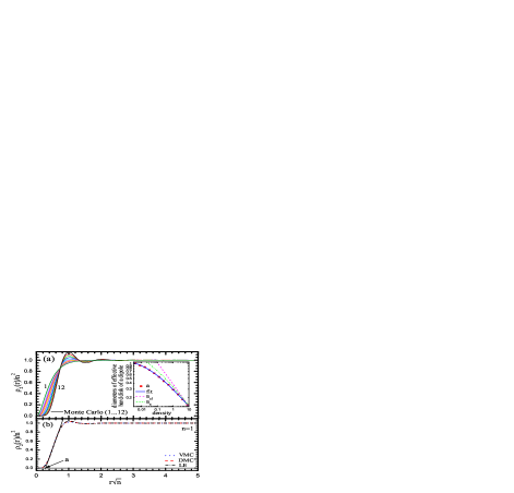
Figure 4: (a) Exciton pair distribution function at $T=0$ for different densities $n=2^{i-9}$ ($i=1,2...12$). The inset shows density dependences for the diameter $a$ of the dipole effective hard disk, polynomial fitting curve (22), energy dependent dipole scattering length, $a_{s}$ (23), and classical turning point for the dipole potential, $a_{cl}=1/\sqrt[\mbox{\small 3}\!]{2E_{0}/N}$. (b) VMC and DMC results and their linear extrapolation (LE) for pair distribution function at $n=1$ (curves practically coincide). The arrow clarifies the definition of the diameter $a$ of the dipole effective hard disk.

At high densities ($n\geq 1/8$), the pair distribution function exhibits a clearly pronounced hump, corresponding to a short-range order. At very high densities, there are also weaker humps. This is indicative of strong correlations in 2D dipolar exciton system in CQWs in the low-temperature exciton phase studied in revT ; revB ; T ; B ; M .

The inset of Fig. 4(a) shows the density dependence of the diameter $a$ of the effective hard disk of a dipole. We define this diameter as the distance from the origin to the point of intersection of the short-wavelength tangent line to the pair distribution function with the abscissa axis (see Fig. 4(b)). The calculated points are described well (within 2%) by the following polynomial fitting curve:

$$a=a_{a}\exp(b_{a}\ln n+c_{a}\ln^{2}n+d_{a}\ln^{3}n),$$ (22)

where $a_{a}=0.293$, $b_{a}=-0.324$, $c_{a}=-0.0123$ and $d_{a}=0.00096$.

The calculation of the diameter of the effective hard disk makes it possible to evaluate the influence of the internal exciton structure, which is not taken into account in the model of dipolar excitons. If the exciton diameter is smaller than the diameter $a$ of the dipole effective hard disk, the neglect of the internal structure of dipolar excitons is justified. This is connected with the fact that the probability density of one exciton to be at a distance of $r<a$ from another exciton, which is proportional to $\rho_{2}(r)$, is small (Fig. 4(b)).

The average electron-hole distance $a_{eh}$ in the exciton can be taken to estimate the exciton diameter in GaAs. In structure (1), which consists of GaAs CQWs revT ; T , the average distance $a_{eh}=17$ nm; therefore, for the dimensional exciton density $n<3.2\cdot 10^{10}$ cm^-2, $a_{eh}<a$.

If the exciton diameter is greater than $a$, the internal structure somewhat affects the microscopic properties of dipolar excitons. However, up to densities $n$ corresponding to the boundary between the strong and weak coupling regimes, where the dipole barrier ceases to suppress exchange effects (see Sections I and II), this influence still can be neglected.

In structure (1) revT ; T , at the maximal exciton density $5.17\cdot 10^{10}$ cm^-2 (see Eq. (6)), corresponding to the boundary between the strong and weak coupling regimes, we find $a=14.2$ nm $\approx 0.84a_{eh}$.

Finally, in the inset of Fig. 4(a), we present the scattering length $a_{s}=a_{s}(p)$,

$$a_{s}(p)=a_{s}^{a}\exp(b_{s}^{a}\ln p+c_{s}^{a}\ln^{2}p+d_{s}^{a}\ln^{3}p)$$ (23)

of two dipoles with the relative momentum $p\sim\sqrt{2E_{0}/N}$ and the energy of order of $E_{0}/N$. Here, $a_{s}^{a}=0.68845$, $b_{s}^{a}=-0.45897$, $c_{s}^{a}=-0.03098$, and $d_{s}^{a}=0.002096$. Fit (23) is based on the calculation of Ref.  ABKLas and, at $0.1\leq p\leq 20$ (i.e., at $1/340\leq n\leq 9.3$; see Eq. (11)), coincides with it within 0.04%. It is seen from the inset that, at low densities, the diameter $a$ of the effective hard disk is smaller than the scattering length $a_{s}$.

III.4 The static structure factor. The sound velocity

The structure factor of 2D dipolar excitons is defined via the Fourier transform of their pair distribution function $\rho_{2}({\bf r})=\langle\hat{\rho}({\bf r})\hat{\rho}(0)\rangle$ as

$$S({\bf p})=1+\int e^{-i{\bf pr}}(\rho_{2}({\bf r})/n-n)d{\bf r}.$$ (24)

For a system with a finite size $L$ and with periodic boundary conditions, this parameter is a discrete function of the momentum (${\bf p}=(2\pi/L){\bf n}$, where ${\bf n}=\{n_{x},n_{y}\}$ is the integer-valued vector). However, the experiment is, as a rule, interested in large 2D Bose condensed exciton systems with a rather large exciton number and a complex boundary. For their description, it is convenient to use the expression for the structure factor in the corresponding infinite system.

For momenta $p\gg 2\pi/L$, the form for the structure factor of the infinite system, $S({\bf p})\equiv S(p)$, can approximately be obtained from Eq. (24) for a flat trap of the size $L$ (with a number of excitons equal to, e.g., $N=100$), if Eq. (24) is smoothed by integrating over the polar angle,

$$S(p)=1+\int J_{0}(pr)(\rho_{2}(r)/n-n)2\pi rdr,\;\;\;\;p\gg 2\pi/L.$$ (25)

Here, it is taken into account that $\int_{0}^{2\pi}e^{-ix\cos\varphi}d\varphi=2\pi J_{0}(x)$, where $J_{0}(x)$ is the zeroth-order Bessel function. For a density of, e.g., $n=1$, the difference between smoothed structure factors (25) determined for two values of the exciton number, $N=100$ and $N=200$, does not exceed 0.35%. Consequently, smoothed form (25) for the structure factor approximates well this parameter for the infinite system at $p\gg 2\pi/L$.

However, at very small momenta, $p\lesssim 2\pi\hbar/L$, at which effects of the finiteness of the system manifest themselves, smoothing (25) does not yield the correct result for infinite systems. To obtain the correct result for an infinite system at such small momenta, it is necessary to join Eq. (25) with the long-wavelength hydrodynamic asymptotics for the structure factor known from the general theory. For higher accuracy, we will use the third-order long-wavelength asymptotics in momentum Khalatn ,

$$S(p)=sp(1+\gamma p^{2}),\;\;\;\;p\lesssim 2\pi/L,$$ (26)

valid on hydrodynamic scales $p\ll p_{0}\equiv 1/r_{0}\sim\sqrt{n}$ (see Section III.2). Here, $s=const>0$ is the parameter responsible for the long-wavelength behavior of the structure factor, while the quantity $\gamma=const$ determines the third order in $p$. The smooth joining (the coincidence of the functions and of their first derivative) of the smoothed structure factor (25) and the long-wavelength asymptotics (26) at intermediate momenta $2\pi/L\ll p\ll p_{0}$ turns out to make it possible to rather precisely determine the value of $s$. For $N=100$, the prediction for $s$, $s=1/\sqrt{8\pi n\zeta}$, based on the polynomial fitting (11) to the energy (see Eqs. (9)-(14), (27), (28)) yields the difference from the macroscopic limit that is less than by 0.08%. This is indicative of the adequacy of our approximations.

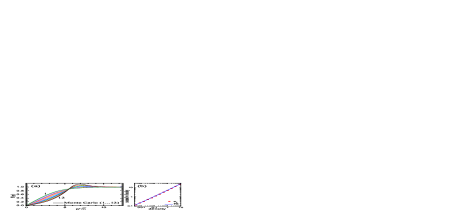
Figure 5: (a) Exciton structure factor at $T=0$ for different densities $n=2^{i-9}$ ($i=1,2...12$). (b) Sound velocity determined from the slope of the structure factor (squares) and based on fitting (11) to the energy (solid curve) as a function of the density.

Figure 5(a) depicts the structure factor of the corresponding infinite system calculated by Eqs. (25) and (26) for different densities. At high exciton densities ($n\geq 1/8$), the curves exhibit a hump corresponding to a short-range order. At densities $1/4\lesssim\bar{n}\lesssim 4$, this hump is clearly seen. This testifies to strong correlations in the dense gas of 2D dipolar excitons in CQWs studied in revT ; revB ; T ; B ; M .

Figure 5(b) shows the dependence of the sound velocity $c_{s}$ in the collisionless regime on the density, which we determine from hydrodynamic considerations from the parameter $s$,

$$c_{s}=\frac{1}{2s}$$ (27)

(see Eq. (29) below). The calculated points for $c_{s}$ fall well on the curve corresponding to the expression of this quantity via the adiabatic compressibility,

$$c_{s}=\sqrt{n/\chi}=\sqrt{2\pi n\zeta}$$ (28)

(the dimensionless adiabatic compressibility $\zeta$ is determined by Eqs. (9), (10), and (14) from fitting (11) to the energy; see Section III.1). This indicates that our DMC simulation is internally consistent.

III.5 The excitation spectrum. Characteristic microscopic scales of the system

In the collisionless regime, the gas phase of the Bose system is known to have only one spectral branch. Therefore, the spectrum of elementary excitations of Bose condensed 2D dipolar excitons in an infinite system at $T=0$ can approximately be calculated by the Feynman formula FF ,

$$\varepsilon_{p}=\frac{p^{2}}{2S(p)}.$$ (29)

which is valid in the long-wavelength (hydrodynamic) range ($r\gg r_{0}$, $p\ll p_{0}$), where the excitation spectrum corresponds to phonons. Approximately, we have (see Section III.4) $S(p)\approx sp(1+\gamma p^{2})$ and $\varepsilon_{p}\approx c_{s}p(1-\gamma p^{2})$. Formula (29) is also true in the short-wavelength range corresponding to an ideal gas ($r\ll r_{IG}$, $p\gg p_{IG}\equiv 1/r_{IG}$), where $S(p)\approx 1$ and $\varepsilon_{p}\approx p^{2}/2$. However, on intermediate scales ($r_{IG}\ll r\ll r_{0}$, $p_{IG}\gg p\gg p_{0}$), the Feynman formula (29) is quantitatively not valid. Nevertheless, it still can be used for qualitative estimates. The details are discussed in Appendix B.

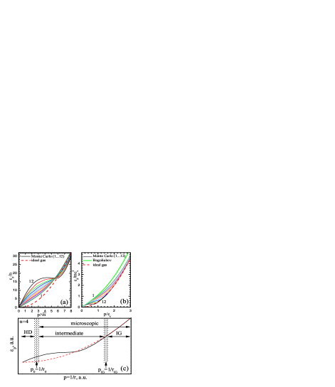
Figure 6: (a) Excitation spectrum at $T=0$ for different densities $n=2^{i-9}$ ($i=1,2...12$). (b) Comparison of the excitation spectra with the Bogolyubov shape. (c) Excitation spectrum for the density $n=4$ (solid curve) and the spectrum of the ideal gas (dashed curve). The hydrodynamic (HD; $r\gg r_{0}$, $p\ll p_{0}$), ideal-gas (IG; $r\ll r_{IG}$, $p\gg p_{IG}$), intermediate ($r_{0}\gg r\gg r_{IG}$, $p_{0}\ll p\ll p_{IG}$), and microscopic ($r\ll r_{0}$, $p\gg p_{0}$) ranges are shown.

In Figs. 6(a) and 6(b), the excitation spectra in an infinite gas of 2D dipolar excitons analytically calculated by Eq. (29) for different densities are shown. It is seen that, in the entire density range used in the calculations, the excitation spectrum is far from the Bogolyubov shape $\varepsilon_{p}^{B}=\sqrt{p^{4}/4+c_{s}^{2}p^{2}}$ (although, at low densities, it qualitatively resembles the Bogolyubov spectrum). At high densities ($1/4\lesssim\bar{n}\lesssim 4$), effects of strong correlations are clearly seen. At the maximal density used in the calculation, $n=8$, a roton minimum appears in the spectrum.

The ranges of long-wavelength (hydrodynamic), short-wavelength (ideal-gas), intermediate, and microscopic scales are clearly seen in Fig. 6(c). The diagrams of the long-wavelength, intermediate, and microscopic ranges were presented above in Fig. 3(d) (see Section III.2).

III.6 Temperature dependence of the local superfluid density. Quasicondensation and BKT transition temperatures

In the quasicondensed Popov phase of excitons far from the crossover between the quasi-classical regime and the quasicondensed phase, elementary excitations form a nearly ideal gas. In this case, the temperature dependence of the fraction of the local (vortex-unrenormalized VR ) superfluid component of quasicondensed 2D dipolar excitons can approximately be calculated by the Landau formula AGD ,

$$\frac{n_{l}(T)}{n}=1+\int\frac{p^{2}}{2}\frac{dn(\varepsilon_{p}^{T})}{d\varepsilon_{p}^{T}}\frac{pdp}{2\pi n}g_{ex},\;\;\;\;T_{q}-T\sim T_{q}.$$ (30)

Here, $n_{l}$ is the local superfluid exciton density (in the $g_{ex}$ spin degrees),

$$n(\varepsilon_{p}^{T})=\frac{1}{e^{\varepsilon_{p}^{T}/T}-1}$$ (31)

is the Bose distribution of the ideal gas of elementary excitations with the spectrum $\varepsilon_{p}^{T}$ at the exciton temperature $T$, and $T_{q}$ is the estimate for the temperature of quasicondensation crossover, at which the local superfluid component and the local long-range order [57] vanish gradually.

The global superfluid component (which takes into account the vortex renormalization jc061181 ; VR ) was calculated in LKW . To calculate the local component, one can set $\varepsilon_{p}^{T}\approx\varepsilon_{p}^{T=0}=\varepsilon_{p}$ in Eqs. (30) and (31). The details of the calculation of the local superfluid component are discussed in Appendix B.

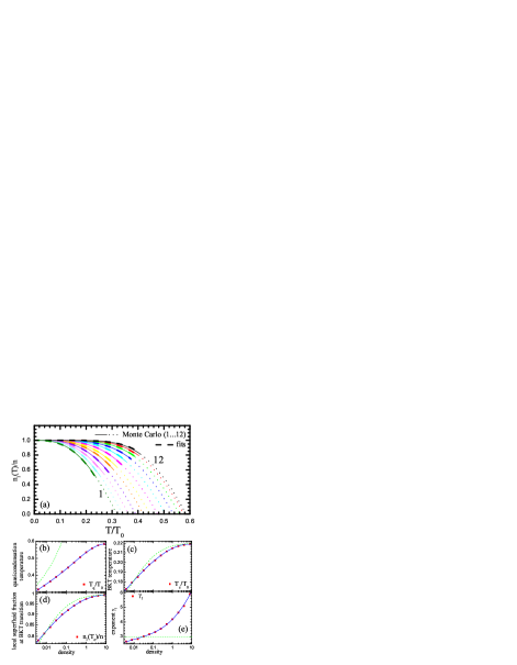
Figure 7: (a) Temperature dependence of the local superfluid exciton fraction in the $g_{ex}=4$ spin degrees for different densities $n=2^{i-9}$ ($i=1,2...12$) (solid curves), low-temperature power-law fitting curves determined by Eq. (33) (dashed curves); and extrapolation to the range of the quasicondensed crossover (dotted curves). (b-d) Density dependences (squares) for (b) the quasicondensation temperature $T_{q}$, (c) the BKT transition temperature $T_{c}$, and (d) the local superfluid fraction at $T=T_{c}$; solid and dashed curves correspond to the polynomial fitting and to phonon-model calculation, respectively. (e) Exponent $\gamma_{l}$ in Eq. (33) as a function of the density: (squares) the fit for each density, (solid curve) the general fitting by Eq. (34), and (dashed curve) the calculation within the phonon model.

The dependence $n_{l}(T)/n$ analytically calculated by means of Eqs. (29)-(31) with $\varepsilon_{p}^{T}=\varepsilon_{p}$ at different densities is shown in Fig. 7(a), where the quantity

$$T_{0}=g_{ex}T_{deg}=2\pi n\;\;\;\;(g_{ex}=4\mbox{ in GaAs}).$$ (32)

denotes the degeneracy temperature for the corresponding spin-polarized excitons.

In the temperature range $0<T<1.2T_{c}$, with an error less than 0.003, this calculation of the local superfluid fraction coincides with the following power-law fitting curve:

$$n_{l}(T)/n=1-(1-n_{l}(T_{c})/n)(T/T_{c})^{\gamma_{l}},$$ (33)

$$\gamma_{l}=a_{l}^{\gamma}+b_{l}^{\gamma}\ln n+c_{l}^{\gamma}\ln^{2}n+d_{l}^{\gamma}\ln^{3}n,$$ (34)

where $a_{l}^{\gamma}=4.186$, $b_{l}^{\gamma}=0.5825$, $c_{l}^{\gamma}=0.0941$, and $d_{l}^{\gamma}=0.00706$, while $T_{c}<T_{q}$ is the temperature of the BKT superfluid transition Berezinskii ; jc061181 ; jc071046 , at which the global superfluid component in the infinite system vanishes jump-wise jc061181 ; rl391201 . For $T_{c}$, we use the equation jc061181 ; rl391201 (see also Appendix B)

$$T_{c}=\frac{\pi n_{l}(T_{c})}{2\tilde{\epsilon}},$$ (35)

in which the dielectric permittivity $\tilde{\epsilon}$ of vortex pairs at the BKT transition can be taken from the 2D $x$-$y$ model ($\tilde{\epsilon}=1.1349\pm 0.0005$; see LKW ).

In Figs. 7(b)-(d), we present the analytically calculated points (denoted by squares) for the temperatures of quasicondensation, $T_{q}$ (see Appendix B), and of the superfluid BKT transition, $T_{c}$, as well as for the local superfluid fraction, $n_{l}(T_{c})/n$, at the BKT transition in the infinite system. These points fall very well on the corresponding polynomial fitting curves (within the limits 0.0025, 0.0005, and 0.0025, respectively),

$$T_{q}/T_{0}=a_{q}^{T}+b_{q}^{T}\ln n+c_{q}^{T}\ln^{2}n+d_{q}^{T}\ln^{3}n+e_{q}^{T}\ln^{4}n,$$ (36)

$$T_{c}/T_{0}=a_{c}^{T}+b_{c}^{T}\ln n+c_{c}^{T}\ln^{2}n+d_{c}^{T}\ln^{3}n,$$ (37)

$$n_{l}(T_{c})/n=a_{c}^{l}+b_{c}^{l}\ln n+c_{c}^{l}\ln^{2}n+d_{c}^{l}\ln^{3}n.$$ (38)

Here, $a_{q}^{T}=0.5344$, $b_{q}^{T}=0.038$, $c_{q}^{T}=-0.00395$, $d_{q}^{T}=-0.001146$, and $e_{q}^{T}=-0.000086$; $a_{c}^{T}=0.2146$, $b_{c}^{T}=0.00414$, $c_{c}^{T}=-0.000877$, and $d_{c}^{T}=-0.0000446$; $a_{c}^{l}=0.9745$, $b_{c}^{l}=0.0188$, $c_{c}^{l}=-0.00398$, and $d_{c}^{l}=-0.000202$.

According to our results, the phonon model, which is widespread in the literature SFB ; LB (in which $\varepsilon_{p}\equiv c_{s}p$), describes rather well the temperature of the BKT transition (Fig. 7(c)) but fails to adequately describe the temperature of the quasicondensation crossover (Fig. 7(b)). (The phonon model does not take into account the roton bend of the spectra on intermediate scales (see Figs. 6(a),(c)), which makes the main contribution at high densities and $T\sim T_{q}$.)

It is important that, at high densities ($1/4\lesssim\bar{n}\lesssim 4$), the local superfluid fraction at the BKT transition, $n_{l}(T_{c})/n$, is close to unity. This is inductive of strong correlations in the dense 2D dipolar exciton gas in CQWs revT ; revB ; T ; B ; M (see also Ref. nl=n ).

In addition, for the spin-depolarized dense 2D dipolar exciton gas in GaAs ($g_{ex}=4$), the temperature of quasicondensation $T_{q}\sim 0.5T_{0}$ (see Fig. 7(b)) is approximately two times higher than the temperature of degeneracy $T_{deg}=T_{0}/g_{ex}=0.25T_{0}$ (see Eq. (32)), whereas the BKT transition temperature $T_{c}\approx 0.2T_{0}$ (see Fig. 7(c)) is only slightly lower than $T_{deg}$. This strongly differs from models widespread in the literature of ideal and weakly correlated 2D exciton gases in QWs for which these temperatures are logarithmically small compared to the degeneracy temperature $T_{deg}$ b3704936 .

Therefore, the condensed state of 2D dipolar excitons in CQWs and SQWs can be experimentally obtained much simpler than in the case of weakly correlated excitons.

IV A harmonic trap at $T=0$

Modern experimental methods are capable of harmonic trapping of 2D dipolar excitons in the plane of a quantum well. This trapping can be obtained with the help of an inhomogeneous compression of the sample, caused by the pressure of a tip on its surface ss134037 ; rl970103 , as well as with the help of an inhomogeneous electric field in electrostatic traps revT ; b7400409 ; jl800185 ; mj360940 ; a0990604 ; prb076085304 .

In the latter experiments on Bose condensation of excitons, their number in a harmonic trap is large, $N\gg 1$ revT ; ss134037 ; rl970103 ; jl800185 . In this case, the phonon microscopic length scale $r_{0}\sim 1/\sqrt{n(0)}$ (see Eq. (20); $n({\bf R})$ is the total exciton profile in the trap) proves to be significantly smaller than the trap size $L_{TF}\sim\sqrt{N/n(0)}$ ($L_{TF}=\sqrt{2N/\pi n(0)}$ is the Thomas-Fermi (TF) radius). In the calculated density range, other microscopic scales ($\xi$, $r_{IG}$, $a$, etc.) are even smaller than $r_{0}$ (see Section III). Therefore, microscopic properties of excitons in a trap can be formed on local scales, along which the potential of the trap varies continuously.

Moreover, if the exciton number $N$ in a trap is substantially greater than $4\pi^{2}\approx 40$ the hydrodynamic range $p\ll 1/r_{0}\sim\sqrt{n(0)}$ considerably exceeds the momentum discreteness step $2\pi/L_{TF}\sim 2\pi\sqrt{n(0)/N}\ll\sqrt{n(0)}$, which is determined by boundary effects in the homogeneous system with the size $L=L_{TF}$ (see Sections III.2 and III.4). Therefore, in the exciton system in a large trap containing $N\gg 40$ excitons, the sound range of momenta, $2\pi/L_{TF}\ll p\ll 1/r_{0}$ does exist and is not masked by finite-size effects, arising on scales $p\lesssim 2\pi/L_{TF}$.

Therefore, a sufficiently large harmonically trapped 2D dipolar exciton system at $T=0$ can be fairly well described in the local density approximation (LDA) LDA . In this approximation, the local microscopic exciton properties near the point ${\bf R}$ of the trap are approximately replaced by the properties of the corresponding homogeneous system with the density $n$ equal to the exciton density $n({\bf R})$ in the trap at the point ${\bf R}$.

Thus, within the framework of the LDA, the total exciton density profile in a (symmetric) trap $n(R)$ is determined from the TF equation, which, at $T=0$, takes the form

$$V(R)+\mu(n(R))=\mu,$$ (39)

where $V(R)=(m/2)\omega_{ho}^{2}R^{2}$ is the potential of the trap with the oscillator frequency $\omega_{ho}$, $\mu$ is the chemical potential of excitons in the trap counted from the exciton band edge, and $\mu(n(R))$ is the local chemical potential of excitons in the trap equal to their chemical potential in the homogeneous system with the density $n=n(R)$.

The density of exciton Bose condensate at $T=0$ in a harmonic trap can be calculated in the LDA as

$$n_{0}(R)=n_{0}(n(R)),$$ (40)

where $n_{0}(n(R))$ is the Bose condensate density in the homogeneous system with the total density $n=n(R)$.

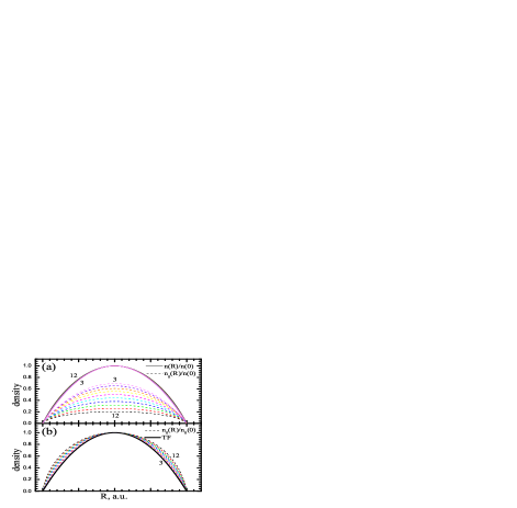
Figure 8: (a) Total ($n(R)/n(0)$) and Bose condensate ($n_{0}(r)/n(0)$) exciton profiles in a harmonic trap in the LDA at $T=0$ and $\zeta_{e}^{\prime}\equiv 2e^{2}D/\varepsilon=10$ for different densities at the center ($n(0)=2^{i-9}$, $i=3,4...12$). (b) Comparison of the Bose condensate profiles at different $n(0)$ with the Thomas-Fermi inverted parabola.

Figure 8(a) shows the total and Bose condensate exciton profiles in a harmonic trap at $T=0$ analytically calculated in the LDA for different densities $n(0)$ at the trap center. The quantities $\mu(n)$ and $n_{0}(n)$ in the infinite homogeneous system were approximately calculated using the corresponding fits (11) and (19) (see also (8) and (9)) for the homogeneous finite system consisting of $N=100$ excitons.

It is clearly seen from this figure that, at $\zeta_{e}^{\prime}\equiv\mu_{e}/T_{0}\equiv 2e^{2}D/\varepsilon=10$, the total density $n(R)$ for all $n(0)$ nearly ideally fall on the profile of the inverted TF parabola (see Fig. 8(a)),

$$n(R)\approx n(0)(1-R^{2}/L_{TF}^{2})\theta(L_{TF}-R)$$ (41)

where $\theta(x)=0$ at $x<0$ and $\theta(x)=1$ at $x>0$. However, this fact is determined not so much by a weak nonlinearity of the collisional contribution to the chemical potential as by a large value of the electrostatic contribution $\mu_{e}=\zeta_{e}^{\prime}T_{0}=10T_{0}$, which is linear in the density (see Eq. (32)). (The values of the electrostatic contribution to the chemical potential $\zeta_{e}^{\prime}\approx 10$ were realized in experiments revT ; revB ; T ; B ; M ; rl970103 ; b7400409 ; transp .)

However, the shape of the Bose condensate profile $n_{0}(R)$ at high densities ($1/4\lesssim\bar{n}\lesssim 4$) appreciably differs from that of the inverted parabola $n_{0}(0)(1-R^{2}/L_{TF}^{2})\theta(L_{TF}-R)$, Fig. 8(b). This is evidence in favor of strong correlations in the dense 2D dipolar exciton gas.

Note that the LDA makes it possible to predict the frequencies of collective oscillations of the compression mode, when the excitation is caused by a sharp change in the frequency of the trapping potential a7200620 . The frequency of this mode depends on the particular form of the two-particle interaction (in contrast to the mode that is caused by the displacement of the center of mass and that depends only on the trap frequency). This makes it possible to experimentally investigate the equation of state (see Eq. (11)). Another important quantity measured in experiment is the release energy. A rapid switching-off of a trap turns the trapping potential to zero but practically has no effect on the kinetic energy and the part of the potential energy related to the pair interaction. The released energy can be measured during the spread. Using the LDA, it is possible to estimate the release energy a7200620 .

V The possibility of the experimental observation of strong exciton correlations

Effects of strong correlations in a dense 2D dipolar exciton gass in CQWs can be found upon observation of the particular features of exciton luminescence in a longitudinal magnetic field.

Indeed, in the absence of a magnetic field, according to the momentum conservation for one-photon exciton recombination, the momentum $p$ of a recombining exciton is equal to the projection of the momentum of an emitted photon onto the QW plane, $(\hbar\omega/c_{0})\sin\theta$. Here, $\theta$ is the angle between the emitted photon and a normal in a vacuum, $c_{0}$ is the light velocity in a vacuum, and $\omega$ is the photon frequency (now we pass to the ordinary, dimensional, units). However, if a longitudinal magnetic field $H_{\parallel}$ is applied to the system, the dispersion curve $\varepsilon_{p}$ of 2D dipolar excitons is shifted by the quantity $p_{H}=eDH_{\parallel}/c_{0}$ BH (this effect is equivalent to the excitation of diamagnetic currents in a system of coupling $e$ and $h$ by a longitudinal magnetic field b6502304 that was described in LY ). As a result, the relation between the emitted-photon angle $\theta$ and the recombined-exciton momentum $p$ takes the form

$$(\hbar\omega/c_{0})\sin\theta=|{\bf p}-{\bf p}_{H}|.$$ (42)

If we are interested in luminescence along the normal ($\theta=0$), then, $p=p_{H}$ (see Eq. (42)), so, $\varepsilon_{p}=\varepsilon_{p_{H}}$. Hence, for the spectral-angular luminescence along the normal in the field $H_{\parallel}$ at $T=0$ we obtain

$$I_{\theta=0}^{H}(\omega)=I_{\theta=0}^{H}\delta(\omega-\Omega+\varepsilon_{p_{H}}/\hbar),\;\;\;\;p_{H}\gg p_{T},$$ (43)

where $I_{\theta=0}^{H}$ is the spectrally integrated angular luminescence along the normal in the field $H_{\parallel}$, $\Omega$ is the exciton resonance frequency (for the luminescence at $H_{\parallel}=0$ and $\theta=0$), and $p_{T}=T/c_{s}$ is the characteristic thermal momentum of Bose condensed excitons, which separates the ranges of thermal $p\ll p_{T}$ and zero-temperature $p_{T}\ll p\ll p_{0}$ quasicondensate phase fluctuations Popov .

Eq. (43)) shows that the measurement of the luminescence line redshift Butovblueshift $\varepsilon_{p_{H}}/\hbar$ in the magnetic field $H_{\parallel}=c_{0}p_{H}/eD$ makes it possible to directly determine the excitations spectrum $\varepsilon_{p}$. At $D=12.3$ nm, $m=0.22m_{0}$, $\varepsilon=12.5$ revB ; B , $n=2\cdot 10^{10}$ cm^-2, and $H_{\parallel}=8$ T, we have

$$p_{H}/\hbar=1.49\cdot 10^{6}\mbox{ cm}{}^{-1}=10.5\sqrt{n}\approx p_{IG}/\hbar$$

(see Section II and Fig. 3(d)). Therefore, in structure (2) revB ; B containing an exciton gas with the density $n=2\cdot 10^{10}$ cm^-2, the field $H_{\parallel}=8$ T covers both the sound (hydrodynamic, $p\ll p_{0}$) and the intermediate ($p_{0}\ll p\ll p_{IG}$) spectral ranges (see Fig. 6(c)). In this case, at $T=0.2T_{0}=1$ K, $m=0.22m_{0}$, and $\zeta=3.7$ (see Fig. 2(b) and Sections II, III.1), the thermal momentum $p_{T}$ corresponds to the field

$$H_{\parallel}^{T}=\frac{c_{0}T}{eD}\sqrt{\frac{m}{\zeta T_{0}}}\approx 0.2\mbox{ T}.$$

Knowing the slope of the measured spectrum $\varepsilon_{p_{H}}$, one can calculate the sound velocity $c_{s}\approx\varepsilon_{p_{H}}/p_{H}$ ($p_{H}\ll p_{0}$; see Fig. 6(a)). This yields the dimensionless adiabatic compressibility (see (28))

$$\zeta=m^{2}c_{s}^{2}/2\pi\hbar^{2}n.$$

Alternatively, the adiabatic compressibility $\zeta$ can be found from the measurement of the spectrally integrated luminescence along the normal in the magnetic field, $I_{\theta=0}^{H}$.

Indeed, the spectrally integrated luminescence into the solid angle $d\Omega=\sin\theta d\varphi d\theta$ near the normal is connected with the momentum distribution of excitons $n_{p_{H}}\equiv\int e^{-\frac{i}{\hbar}{\bf p}_{H}{\bf r}}\rho_{1}({\bf r})d{\bf r}$ (i.e., the number of excitons with the momentum $p_{H}$) by the following relation:

$$I_{\theta=0}^{H}d\Omega=\kappa\frac{\hbar\omega}{\tau_{0}}n_{p_{H}}\frac{d{\bf p}_{H}}{(2\pi\hbar)^{2}}.$$ (44)

Here, $\tau_{0}$ is the lifetime of an isolated spin-depolarized exciton in the ground state and $\kappa=1/2$ ($\kappa=1$) in the case of the measurement of the luminescence only on one side (on both sides) of the QW plane.

On scales $p_{T}\ll p_{H}\ll p_{0}$ that are the most interesting to us, the momentum distribution at $T=0$ is given by the Fourier transform of Eq. (18),

$$n_{p_{H}}=\frac{n_{0}}{n}\frac{mc_{s}}{2p_{H}},\;\;\;\;p_{T}\ll p_{H}\ll p_{0}.$$ (45)

From Eqs. (44) and (45), we find the sought relation between the angular luminescence along the normal, $I_{\theta=0}^{H}$, and the dimensionless adiabatic compressibility $\zeta$,

$$I_{\theta=0}^{H}=I_{0}\frac{q_{r}^{2}c_{0}}{4\pi eD\sqrt{mT_{0}}}\frac{\sqrt{\zeta}}{H_{\parallel}},\;\;\;\;p_{T}\ll eDH_{\parallel}/c_{0}\ll\hbar\sqrt{n}.$$ (46)

Here, $I_{0}=\kappa(\hbar\Omega/\tau_{0})n_{0}$ is the exciton Bose condensate luminescence at $T=0$. At $n=2\cdot 10^{10}$ cm^-2, $D=12.3$ nm, $T=0.1T_{0}=0.5$ K, $m=0.22m_{0}$, $\varepsilon=12.5$, and $\zeta=3.7$, the momentum range $p_{T}\ll eDH_{\parallel}/c_{0}\ll p_{0}$ in Eq. (46) corresponds to the magnetic-field range

$$\frac{c_{0}T}{eD}\sqrt{\frac{m}{\zeta T_{0}}}\ll H_{\parallel}\ll\frac{c_{0}\hbar\sqrt{n}}{eD},$$

or 0.1 T $\ll H_{\parallel}\ll$ 0.75 T.

The luminescence intensity of the Bose condensate at $T=0$ appearing in Eq. (46) can be approximately calculated as the contribution of thermal phase fluctuations to the quasicondensate luminescence at low temperatures (see Eq. (44)),

$$I_{0}\approx\int_{0}^{p_{T}}I_{\theta=0}^{H}\frac{2\pi p_{H}dp_{H}}{q_{r}^{2}}=\kappa\frac{\hbar\Omega}{\tau_{0}}n_{0},\;\;\;\;T\ll T_{q},$$ (47)

where $q_{r}=\hbar\Omega/c_{0}$ is the radiation bandwidth in a vacuum. Here, it is taken into account that the exciton gap $\hbar\Omega\sim 1$ eV considerably exceeds all characteristic energy scales for excitons $\varepsilon_{p_{H}},T\lesssim 1$ meV $\ll\hbar\Omega$, so, $\hbar\omega\approx\hbar\Omega$. It is also taken into account that $dp_{H}=q_{r}d\sin\theta=q_{r}d\theta$ at $p_{H}=p$ and $\theta=0$ (see Eq. (42)). (Eq. (47) can be obtained by extending the method described in Appendix A to the case $T\neq 0$, see Refs. PFCT ; Popov .)

Finally, by measuring the quantity (47), one can find the important parameter of exciton correlations, namely, the Bose condensate density at $T=0$,

$$n_{0}=\frac{1}{\kappa}\frac{\tau_{0}}{\hbar\Omega}I_{0}.$$

VI Conclusion

By means of the ab initio simulation and analytical calculations, we studied in detail the microscopic properties of Bose condensed superfluid 2D dipolar excitons in QWs. For a homogeneous exciton system, we numerically calculated the ground-state energy, the one-body density matrix, and the pair distribution function. Based on these numerical calculations for the homogeneous system, we analytically found the structure factor, the excitation spectrum, the Bose condensate density, the temperature dependence of the local superfluid density, the chemical potential, the adiabatic compressibility, the sound velocity, and the characteristic microscopic length scales (the phonon scale, the healing length, the scattering length, the diameter of the effective hard disk of a dipole, etc.), as well as the quasicondensation crossover and Berezinskii-Kosterlitz-Thouless transition temperatures. For a harmonic trap with a large excton number, we analytically calculated the total and Bose condensate profiles.

We showed that, in all experiments on Bose condensation performed at present, 2D dipolar excitons in coupled QWs prove to be strongly correlated. As a consequence, exciton Bose condensation and superfluidity can experimentally be achieved much easily than this is predicted by the models of an ideal and weakly correlated exciton gases.

The results obtained for the ground-state energy $E_{0}/N$, chemical potential $\mu=\mu_{i}+\mu_{e}$, the adiabatic compressibility $\chi$, the sound velocity $c_{s}$, the excitation spectrum $\varepsilon_{p}$, and the Bose condensate $n_{0}$ and local superfluid $n_{l}(T)$ densities, as well as for the characteristic microscopic phonon length scale $r_{0}$, can be used as reference data in construction of quantitative hydrodynamic theory of the optical properties of 2D dipolar excitons in QWs, in particular, of their luminescence, coherence, and nonlinear effects.

Appendix A Long-wavelength hydrodynamic asymptotics for the one-body density matrix

On long-wavelength scales ($r\gg r_{0}$), the one-body density matrix (16) of Bose condensed 2D dipolar excitons at $T=0$ can be calculated within the framework of the hydrodynamic method in quantum field theory PFCT ,

$$\rho_{1}({\bf r})=Ce^{-\langle(\hat{\varphi}({\bf r})-\hat{\varphi}(0))^{2}/2\rangle}=n_{0}e^{\langle\hat{\varphi}({\bf r})\hat{\varphi}(0)\rangle},\;\;\;\;r\gg r_{0}.$$ (48)

Here, $\hat{\varphi}({\bf r})$ is the phase of the exciton field operator $\hat{\Psi}({\bf r})$ ($\hat{\Psi}({\bf r})=e^{i\hat{\varphi}({\bf r})}\sqrt{\hat{\rho}({\bf r})}$), which satisfies the commutation relation $[\hat{\varphi}({\bf r}),\hat{\varphi}({\bf r}^{\prime})]=0$, and $C=n_{0}e^{\langle(\hat{\varphi}(0))^{2}\rangle}=const$ does not depend on ${\bf r}$. We assume that an ultraviolet cutoff is imposed (in this case, the quantities $C$ and $\langle(\hat{\varphi}(0))^{2}\rangle$ diverge in the ultraviolet limit, but, at $r\gg r_{0}$, $n_{0}$ and $\langle\hat{\varphi}({\bf r})\hat{\varphi}(0)\rangle$ are finite in the large-momentum limit).

At $T=0$, the phase-phase correlator $\langle\hat{\varphi}({\bf r})\hat{\varphi}(0)\rangle$ in Eq. (48) can be expressed via the phase-phase Green’s function (in dimensional units),

$$D_{p}^{\varphi\varphi}(\omega)=-i\int\langle\hat{\rm T}[\hat{\varphi}({\bf r},t)\hat{\varphi}(0,0)]\rangle e^{-\frac{i}{\hbar}{\bf pr}+i\omega t}d{\bf r}dt,$$

as follows:

$$\langle\hat{\varphi}({\bf r})\hat{\varphi}(0)\rangle=\frac{1}{L^{2}}\sum\nolimits_{{\bf p}\neq 0}e^{\frac{i}{\hbar}{\bf pr}}\int iD_{p}^{\varphi\varphi}(\omega)\frac{d\omega}{2\pi}.$$ (49)

where $\hat{\rm T}$ is the chronological operator.

In the hydrodynamic (long-wavelength) approximation, in which the hydrodynamic Hamiltonian acquires the form local in time, the function $D_{p}^{\varphi\varphi}(\omega)$ is given by Popov ; PHD

$$D_{p}^{\varphi\varphi}(\omega)=\frac{\hbar m\varepsilon_{p}^{2}/n_{s}p^{2}}{\hbar^{2}\omega^{2}-\varepsilon_{p}^{2}+i\delta},\;\;\;\;p\ll p_{0},$$ (50)

where $n_{s}$ is the global superfluid exciton density (in the $g_{ex}$ spin degrees).

In the calculated density range ($nx_{0}^{2}\leq 8$), excitons are in the gas phase rl980605 . In addition, we neglect the external random potential, which is unavoidably present in heterostructures. In this case, the global superfluid exciton density at $T=0$ coincides with the total density (see jc061181 and Section III.6),

$$n_{s}=n.$$ (51)

From Eqs. (49)-(51) we obtain the following equation for the correlator $\langle\hat{\varphi}({\bf r})\hat{\varphi}(0)\rangle$ at $T=0$

$$\langle\hat{\varphi}({\bf r})\hat{\varphi}(0)\rangle=\frac{1}{L^{2}}\sum\nolimits_{{\bf p}\neq 0}e^{\frac{i}{\hbar}{\bf pr}}\frac{m\varepsilon_{p}}{2np^{2}}=$$

$$=\frac{1}{L^{2}}\sum_{{\bf p}\neq 0}e^{\frac{i}{\hbar}{\bf pr}}\frac{m\varepsilon_{p}}{2np^{2}}-\frac{1}{4N}\sum_{\bf p}e^{\frac{i}{\hbar}{\bf pr}}=$$

$$=\sum_{{\bf p}\neq 0}e^{\frac{i}{\hbar}{\bf pr}}\left(\frac{m\varepsilon_{p}}{2Np^{2}}-\frac{1}{4N}\right)-\frac{1}{4N},$$ (52)

$$r\gg r_{0}.$$

Here, we used the fact that, at $r\gg r_{0}$ (i.e., at ${\bf r}\neq 0$), the $\delta$-like contribution

$$\frac{1}{4N}\sum_{\bf p}e^{\frac{i}{\hbar}{\bf pr}}=\frac{1}{4n}\sum_{\bf n}\delta({\bf r}-{\bf n}L)$$

is zero in a box of a size $L$ (${\bf n}=\{n_{x},n_{y}\}$ is the integer-valued vector).

By substituting (52) into (48) and averaging over the polar angle of the vector ${\bf r}$, we arrive at the sought hydrodynamic equation (17) for the one-body density matrix of Bose condensed 2D dipolar excitons at $T=0$, which, on long-wavelength scales ($r\gg r_{0}$), coincides excellently with our DMC simulation (see Fig. 3(e)).

In conclusion, we note that, in interacting systems with the finite scattering length, the spectrum of excitations $\varepsilon_{p}$, at $p\to\infty$, exponentially approaches the spectrum of the ideal gas $\varepsilon_{p}=p^{2}/2m+O(e^{-p/p_{1}})$ (where $p_{1}=const>0$; see also item (2) in Appendix B). Consequently, at $p\to\infty$, the quantity $m\varepsilon_{p}/2Np^{2}-1/4N$ under the summation sign in (52) is of the order of $O(e^{-p/p_{1}})$. Therefore, Eq. (52) for the phase-phase correlator converges in the ultraviolet limit. This means that the well-known ultraviolet cutoff Popov in quantum-field hydrodynamics at the boundary of the long-wavelength band ($r\sim r_{0}$, $p\sim p_{0}$) proves to be redundant in (52): an infinitely small cutoff suffices to ensure convergence.

However, one should bear in mind that the hydrodynamic (long-wavelength) approximation fails to adequately describe the phase-phase correlator on microscopic scales $r\ll r_{0}$, $p\gg p_{0}$. So, the range $p\gg p_{0}$ is incorrectly taken into account in (52). As a result, the hydrodynamic approach used in this study introduces a certain error in the calculation of the one-body density matrix and, therefore, in the Bose condensate density. However, direct calculation shows that, if a continuous finite ultraviolet cutoff is introduced in (52) at $p\sim p_{0}$, the correction to the Bose condensate density will rapidly vanish at large $N$. The numerical calculation of the sum in (52) shows that, at $N=100$, this correction is of the order of 0.001.

Appendix B Applicability conditions and calculation details

Here, we will discuss subtle aspects of calculations of the excitation spectrum, the local superfluid density, and the quasicondensed and superfluid transition temperatures.

(1) As Boronat et al. showed FF , in strongly correlated systems on intermediate scales, the true spectrum lies lower than the spectrum calculated by the Feynman formula (although, the weaker the correlations, the more exact the Feynman formula). Therefore, in the strong-correlation regime, our calculation of the local superfluid fraction, as well as the quasicondensation $T_{q}$ and the BKT transition $T_{c}$ temperatures is valid only qualitatively.

(2) For simplicity, the excitation spectrum was estimated omitting the effects connected with a large damping of elementary excitations above the endpoint of the spectrum AGD .

(3) The Landau formula is valid only in the collisionless (not hydrodynamic) regime when elementary excitations weakly interact, and their damping is small. This is definitely not the case above the spectrum endpoint $p_{c}$. In a dense system, the spectrum endpoint lies high (see Fig. 6(a) and AGD ), so that the range $p>p_{c}$ is cut in (30) by the Bose exponential (31). At low densities, the spectrum endpoint $p_{c}$ corresponds to smaller frequencies, but a significant damping appears only above the sound range of the spectrum. This range is also cut by the Bose exponential (see (30)-(32) and Figs. 6(a), 7(b)). However, at very low densities $\bar{n}$, where excitons are weakly correlated, the hydrodynamic regime can occur precisely in that range of the spectrum which makes the main contribution to the Landau formula. In this case, Eq. (30) does not hold. However, according to our direct estimation, even at a smallest calculated density of $\bar{n}=1/256$, such a situation is not realized.

(4) In calculation of the local component, we set $\varepsilon_{p}^{T}\approx\varepsilon_{p}^{T=0}=\varepsilon_{p}$ in Eqs. (30) and (31). Indeed, at low temperatures, $T\ll T_{q}$, the Bose exponential (31) leaves in (30) only the contribution from long-wavelength scales, on which $\varepsilon_{p}^{T}\approx c_{s}(T)p\approx c_{s}(0)p\approx\varepsilon_{p}$. At high temperatures, ($T\sim T_{q}$, $T<T_{q}$), owing to the factor $(p^{2}/2)pdp$ in Eq. (30), long-wavelength scales do not contribute. On scales in the range of shorter (microscopic) wavelengths, the spectrum calculated by the Feynman formula is weakly affected by temperature variations. The latter fact was revealed in the course of the Monte Carlo simulation of the pair distribution function and the structure factor in liquid helium up to temperatures so high (4.2 K) as the doubled temperature of the $\lambda$ point, $T_{\lambda}=2.1$ K b2103638 .

(5) The temperature of quasicondensation $T_{q}$ we formally calculate from the condition $n_{l}(T_{q})/n=0$, where $n_{l}(T)/n$ is given by Eq. (30) with $\varepsilon_{p}^{T}=\varepsilon_{p}$. This is an approximate estimate, since, in the range of crossover at temperatures near $T_{q}$, the local superfluidity and the local long-range order vanish, elementary excitations cease to form a nearly ideal gas, and the quantum regime goes to the classical regime.

References

- (1) Yu. E. Lozovik and V. I. Yudson, JETP Lett. 22, 274 (1975); JETP 44, 389 (1976); Yu. E. Lozovik and V. I. Yudson, Solid State Commun. 19, 391 (1976); ibid. 21, 211 (1977); Yu. E. Lozovik and V. N. Nishanov, Phys. Solid State 18, 1905 (1976); Yu. E. Lozovik and A. M. Ruvinsky, JETP 85, 979 (1997).
- (2) A. Filinov, P. Ludwig, Yu. E. Lozovik et al., J. Phys: Conf. Series 35, 197 (2006); P. Ludwig, A. Filinov, M. Bonitz, H. Stolz, Phys. Status Solidi B 243, 2363 (2006).
- (3) S. A. Moskalenko and D. W. Snoke, Bose-Einstein condensation of excitons and biexcitons and coherent nonlinear optics with excitons (Cambridge Univ. Press, Cambridge 2000).
- (4) D. Snoke, Science 298, 1368 (2002); R. Rapaport, G. Chen, J. Phys.: Condens. Matter 19, 295207 (2007); Z. Vörös, V. Hartwell, D. W. Snoke et al., ibid. 19, 295216 (2007); Z. Vörös and D. W. Snoke, Mod. Phys. Lett. B 22, 701 (2008).
- (5) V. B. Timofeev, Phys.-Uspekhi 48, 295 (2005).
- (6) L. V. Butov, Solid State Commun. 127, 89 (2003); J. Phys.: Condens. Matter 16, R1577 (2004); ibid. 19, 295202 (2007).
- (7) A. V. Gorbunov, V. E. Bisti, and V. B. Timofeev, JETP 101, 693 (2005); A. V. Larionov, V. B. Timofeev, J. M. Hvam, and C. Soerensen, ibid. 90, 1093 (2000); JETP Lett. 71, 117 (2000); ibid. 75, 200 (2002); A. V. Larionov and V. B. Timofeev, ibid. 73, 301 (2001); A. V. Larionov, V. B. Timofeev, P. A. Ni et al., ibid. 75, 570 (2002); A. A. Dremin, V. B. Timofeev, A. V. Larionov et al., ibid. 76, 450 (2002); A. V. Gorbunov and V. B. Timofeev, ibid. 83, 146 (2006); A. V. Gorbunov, A. V. Larionov, and V. B. Timofeev, ibid. 86, 46 (2007); A. A. Dremin, A. V. Larionov, and V. B. Timofeev, Phys. Solid State 46, 170 (2004).
- (8) L. V. Butov and A. I. Filin, Phys. Rev. B 58, 1980 (1998); L. V. Butov, C. W. Lai, A. L. Ivanov et al., Nature (London) 417, 47 (2002); C. W. Lai, J. Zoch, A. C. Gossard, and D. S. Chemla, Science 303, 503 (2004); L. V. Butov, A. L. Ivanov, A. Imamoglu et al., Phys. Rev. Lett. 86, 5608 (2001); L. V. Butov, L. S. Levitov, A. V. Mintsev et al., ibid. 92, 117404 (2004); A. T. Hammack, M. Griswold, L. V. Butov et al., ibid. 96, 227402 (2006); S. Yang, A. T. Hammack, M. M. Fogler et al., ibid. 97, 187402 (2006); A. T. Hammack, L. V. Butov, L. Mouchliadis et al., Phys. Rev. B 76, 193308 (2007); M. M. Fogler, S. Yang, A. T. Hammack et al., ibid. 78, 035411 (2008); see also b7500311 .
- (9) V. V. Krivolapchuk, E. S. Moskalenko, and A. L. Zhmodikov, Phys. Rev. B 64, 045313 (2001); V. V. Krivolapchuk, E. S. Moskalenko, A. L. Zhmodikov et al., Solid State Commun. 111, 49 (1999).
- (10) D. Snoke, S. Denev, Y. Liu et al., Nature (London) 418, 754 (2002); R. Rapaport, G. Chen, D. Snoke et al., Phys. Rev. Lett. 92, 117405 (2004).
- (11) D. W. Snoke, Y. Liu, Z. Vörös et al., Solid State Commun. 134, 37 (2005).
- (12) Z. Vörös, D. W. Snoke, L. Pfeiffer, and K. West, Phys. Rev. Lett. 97, 016803 (2006).
- (13) G. Chen, R. Rapaport, L. N. Pfeiffer et al., Phys. Rev. B 74, 045309 (2006).
- (14) Z. Vörös, R. Balili, D. W. Snoke et al., Phys. Rev. Lett. 94, 226401 (2005); J. Rudolph, R. Hey, and P. V. Santos, ibid. 99, 047602 (2007).
- (15) A. V. Gorbunov and V. B. Timofeev, JETP Lett. 84, 329 (2006); V. B. Timofeev and A. V. Gorbunov, J. Appl. Phys. 101, 081708 (2007); V. B. Timofeev, A. V. Gorbunov, and A. V. Larionov, J. Phys.: Condens. Matter 19, 295209 (2007).
- (16) D. S. Petrov, M. Holzmann, and J. V. Shlyapnikov, Phys. Rev. Lett. 84, 2551 (2000).
- (17) R. Zimmermann, Phys. Status Solidi B 243, 2358 (2006); R. Zimmermann and C. Schindler, Solid State Commun. 144, 395 (2007); C. Schindler and R. Zimmermann, Phys. Rev. B 78, 045313 (2008); K. I. Golden, G. J. Kalman, Z. Donko, and P. Hartmann, ibid. 78, 045304 (2008); see also MCLKAW .
- (18) Yu. E. Lozovik and O. L. Berman, JETP 84, 1027 (1997); Phys. Scripta 55, 491 (1997); Yu. E. Lozovik, O. L. Berman, and M. Willander, J. Phys.: Condens. Matter 14, 12457 (2002).
- (19) M. Stern, V. Garmider, V. Umansky, and I. Bar-Joseph, Phys. Rev. Lett. 100, 256402 (2008).
- (20) L. V. Keldysh and Yu. V. Kopaev, Phys. Solid State 6, 2219 (1964); A. N. Kozlov and L. A. Maksimov, JETP 21, 790 (1965); L. V. Keldysh and A. N. Kozlov, JETP 27, 521 (1968).
- (21) P. C. Hohenberg, Phys. Rev. 158, 383 (1967); N. D. Mermin and H. Wagner, Phys. Rev. Lett. 17, 1133 (1966).
- (22) J. W. Kane and L. P. Kadanoff, Phys. Rev. 155, 80 (1967); F. Weling, A. Griffin, and M. Carrington, Phys. Rev. B 28, 5296 (1983).
- (23) V. L. Berezinskii, JETP 32, 493 (1970); ibid. 34, 610 (1971).
- (24) J. M. Kosterlitz and D. J. Thouless, J. Phys. C 6, 1181 (1973).
- (25) J. M. Kosterlitz, J. Phys. C 7, 1046 (1974).
- (26) D. R. Nelson and J. M. Kosterlitz, Phys. Rev. Lett. 39, 1201 (1977).
- (27) V. Bagnato and D. Kleppner, Phys. Rev. A 44, 7439 (1991); W. Ketterle and N. J. van Druten, ibid. 54, 656 (1996).
- (28) G. Vignale and A. H. MacDonald, Phys. Rev. Lett. 76, 2786 (1996); S. Conti, G. Vignale, and A. H. MacDonald, Phys. Rev. B 57, R6846 (1998); A. V. Balatsky, Y. N. Joglekar, and P. B. Littlewood, Phys. Rev. Lett. 93, 266801 (2004); Y. N. Joglekar, A. V. Balatsky, and M. P. Lilly, Phys. Rev. B 72, 205313 (2005).
- (29) O. L. Berman, Yu. E. Lozovik, D. W. Snoke, and R. D. Coalson, Phys. Rev. B 70, 235310 (2004); ibid. 73, 235352 (2006); Solid State Commun. 134, 47 (2005); Physica E 34, 268 (2006); J. Phys.: Condens. Matter 19, 386219 (2007).
- (30) Yu. E. Lozovik and M. Willander, Appl. Phys. A 71, 379 (2000); Yu. E. Lozovik, O. L. Berman, and V. G. Tsvetus, Phys. Rev. B 59, 5627 (1999); JETP Lett. 66, 355 (1997); Yu. E. Lozovik and O. L. Berman, ibid. 64, 573 (1996).
- (31) J. F. Jan and Y. C. Lee, Phys. Rev. B 58, 1714 (1998); Z. G. Koinov, ibid. 61, 8411 (2000); R. Rapaport, G. Chen, S. Simon, Appl. Phys. Lett. 89, 152118 (2006).
- (32) X. Zhu, P. B. Littlewood, M. S. Hibertsen, and T. M. Rice, Phys. Rev. Lett. 74, 1633 (1995); Y. Naveh and B. Laikhtman, ibid. 77, 900 (1996); J. Fernández-Rossier and C. Tejedor, ibid. 78, 4809 (1997); P. Pieri, D. Neilson, and G. C. Strinati, Phys. Rev. B 75, 113301 (2007); T. Hakioglu and M. Sahin, Phys. Rev. Lett. 98, 166405 (2007).
- (33) Yu. E. Lozovik, I. L. Kurbakov, G. E. Astrakharchik et al., Solid State Commun. 144, 399 (2007).
- (34) Yu. E. Lozovik and O. L. Berman, Phys. Scripta 58, 86 (1998); Phys. Solid State 40, 1228 (1998); D. V. Kulakovskii, Yu. E. Lozovik, and A. V. Chaplik, JETP 99, 850 (2004).
- (35) S. De Palo, F. Rapisarda, and G. Senatore, Phys. Rev. Lett. 88, 206401 (2002); A. I. Belousov and Yu. E. Lozovik Eur. Phys. J. D 8, 251 (2000); Yu. E. Lozovik and E. A. Rakoch, Phys. Lett. A 235, 55 (1997); C. Mora, O. Parcollet, and X. Waintal, Phys. Rev. B 76, 064511 (2007).
- (36) G. E. Astrakharchik, J. Boronat, I. L. Kurbakov, and Yu. E. Lozovik, Phys. Rev. Lett. 98, 060405 (2007); see also polmol a.
- (37) Yu. E. Lozovik, I. L. Kurbakov, and G. E. Astrakharchik (to be publ.).
- (38) A. I. Belousov and Yu. E. Lozovik, JETP Lett. 68, 858 (1998); Yu. E. Lozovik, S. Y. Volkov, and M. Willander, ibid. 79, 473 (2004); A. Filinov, M. Bonitz, P. Ludwig, and Yu. E. Lozovik, Phys. Status Solidi C 3, 2457 (2006); G. E. Astrakharchik, J. Boronat, J. Casulleras et al., arXiv:0707.4630.
- (39) A. L. Ivanov, P. B. Littlewood, and H. Haug, Phys. Rev. B 59, 5032 (1999); A. V. Soroko and A. L. Ivanov, ibid. 65, 165310 (2002); S. V. Iordanskii and A. Kashuba, JETP Lett. 73, 479 (2001); A. L. Ivanov, Europhys. Lett. 59, 586 (2002).
- (40) S. I. Shevchenko, Phys. Rev. Lett. 72, 3242 (1994); Phys. Rev. B 56, 10355 (1997); ibid. 57, 14809 (1998); Yu. E. Lozovik and E. A. Rakoch, ibid. 57, 1214 (1998); E. Babaev, ibid. 77, 054512 (2008); T. Iida and M. Tsubota, ibid. 60, 5802 (1999); J. Lumin. 87-89, 241 (2000).
- (41) Yu. E. Lozovik and V. I. Yudson, Solid State Commun. 22, 117 (1977); A. V. Klyuchnik and Yu. E. Lozovik, JETP 49, 335 (1979); J. Phys. C 11, L483 (1978); Yu. E. Lozovik and A. V. Poushnov, Phys. Lett. A 228, 399 (1997). see also V a.
- (42) B. Laikhtman, Europhys. Lett. 43, 53 (1998); P. Stenius, Phys. Rev. B 60, 14072 (1999); L. Mouchliadis and A. L. Ivanov, ibid. 78, 033306 (2008); Yu. E. Lozovik and I. V. Ovchinnikov, ibid. 66, 075124 (2002); JETP Lett. 74, 288 (2001); Solid State Commun. 118, 251 (2001); Yu. E. Lozovik, I. L. Kurbakov, and I. V. Ovchinnikov, ibid. 126, 269 (2003); J. Keeling, L. S. Levitov, and P. B. Littlewood, Phys. Rev. Lett. 92, 176402 (2004).
- (43) L. S. Levitov, B. D. Simons, and L. V. Butov, Phys. Rev. Lett. 94, 176404 (2005); Solid State Commun. 134, 51 (2005); A. Paraskevov and T. Khabarova, Phys. Lett. A 368, 151 (2007); A. A. Chernyuk and V. I. Sugakov, Phys. Rev. B 74, 085303 (2006); V. I. Sugakov and A. A. Chernyuk, JETP Lett. 85, 570 (2007).
- (44) Yu. E. Lozovik, I. L. Kurbakov, and M. Willander, Phys. Lett. A 366, 487 (2007).
- (45) Yu. E. Lozovik, O. L. Berman, and A. M. Ruvinsky, JETP Lett. 69, 616 (1999); see also LB a,PHD b and K. Huang and H.-F. Meng, Phys. Rev. Lett. 69, 644 (1992); M. P. A. Fisher, P. B. Weichman, G. Grinstein, and D. S. Fisher, Phys. Rev. B 40, 546 (1989).
- (46) K. Moon, H. Mori, K. Yang et al., Phys. Rev. B 51, 5138 (1995); K. Park and S. Das Sarma, ibid. 74, 035338 (2006); Yu. E. Lozovik and I. V. Ovchinnikov, JETP Lett. 79, 76 (2004); H. A. Fertig and G. Murthy, Phys. Rev. Lett. 95, 156802 (2005); J. P. Eisenstein and A. H. MacDonald, Nature (London) 432, 691 (2004); J. P. Eisenstein, Science 305, 950 (2004); see also LB b.
- (47) M. Kellogg, J. P. Eisenstein, L. N. Pfeiffer, and K. W. West, Phys. Rev. Lett. 93, 036801 (2004); E. Tutuc, M. Shayegan, and D. A. Huse, ibid. 93, 036802 (2004).
- (48) T. Lahaye, T. Koch, B. Frohlich et al., Nature (London) 448, 672 (2007); A. Griesmaier, J. Werner, S. Hensler et al., Phys. Rev. Lett. 94, 160401 (2005); D. Jaksch, J. I. Cirac, P. Zoller et al., ibid. 85, 2208 (2000); H. Pu, W. Zhang, and P. Meystre, ibid. 87, 140405 (2001); S. Yi and L. You, Phys. Rev. A 63, 053607 (2001); U. R. Fischer, ibid. 73, 031602 (2006); S. Yi and H. Pu, ibid. 73, 061602 (2006); G. E. Astrakharchik, J. Boronat, J. Casulleras et al., ibid. 75, 063630 (2007).
- (49) H. P. Büchler, E. Demler, M. Lukin et al., Phys. Rev. Lett. 98, 060404 (2007); D. DeMille, ibid. 88, 067901 (2002); R. V. Crems, ibid. 96, 123202 (2006); J. M. Sage, S. Sainis, T. Bergeman, and D. DeMille, ibid. 94, 203001 (2005); J. L. Bohn, Phys. Rev. A 63, 052714 (2001); T. Köhler, K. Góral, and P. S. Julienne, Rev. Mod. Phys. 78, 1311 (2006).
- (50) M. Schick, Phys. Rev. A 3, 1067 (1971); Yu. E. Lozovik and V. I. Yudson, Physica A 93, 493 (1978); E. B. Kolomeisky and J. P. Straley, Phys. Rev. B 46, 11749 (1992); A. Yu. Chreny and A. A. Shanenko, Phys. Rev. E 64, 027105 (2001).
- (51) In some observations of structured luminescence rings b7500311 , excitons are weakly correlated. However, we suppose their density to be too low, so, the transition to a collective state does not occur. Indeed, our estimation shows (see Ref. LKW , and Sections II, III.1, III.6)) that, for the blueshift of the luminescence line observed in b7500311 (being of the order of 0.5 meV), the exciton density is cm-2. So, the superfluid crossover temperature in a trap with a size of is K, which is much lower than the exciton temperature K.
- (52) S. Yang, A. V. Mintsev, A. T. Hammack et al., Phys. Rev. B 75, 033311 (2007).
- (53) D. S. Fisher and P. C. Hohenberg, Phys. Rev. B 37, 4936 (1988); see also Popov .
- (54) The local superfluid exciton density (see Section III.6) at the superfluid transition temperature () is small () in 3D systems and in quasi-2D systems with unquantized transverse motion. In (quasi-)2D systems with quantized transverse motion, the inequality at holds true if the correlations are either weak or so strong that the roton minimum is very deep. Therefore, the equality at in 2D systems with quantized transverse motion holds only if correlations are rather strong. In the case of intermediate correlations, the fulfillment of the equality at is worse.
- (55) S. Schmitt-Rink, D. S. Chemla, and D. A. B. Miller, Phys. Rev. B 32, 6601 (1985).
- (56) L. Reatto and G. V. Chester, Phys. Rev. 155, 88 (1967).
- (57) J. Boronat and J. Casulleras, Phys. Rev. B 49, 8920 (1994).
- (58) J. Casulleras and J. Boronat, Phys. Rev. B 52, 3654 (1995).
- (59) G. E. Astrakharchik, J. Boronat, J. Casulleras, I. L. Kurbakov, and Yu. E. Lozovik (to be publ.).
- (60) I. M. Khalatnikov, Introduction to the theory of superfluidity (Benjamin, New York, 1965).
- (61) R. P. Feynman, Phys. Rev. 94, 262 (1954); L. P. Pitaevskii, JETP 4, 439 (1957); J. Boronat, J. Casulleras, F. Dalfovo et al., Phys. Rev. B 52, 1236 (1995).
- (62) V.N. Popov, Functional Integrals in Quantum Field Theory and Statistical Physics (Reidel, Dordrecht, 1983).
- (63) P. Minnhagen, Rev. Mod. Phys. 59, 1001 (1987); Phys. Rev. B 32, 3088 (1985); P. Minnhagen and G. G. Warren, ibid. 24, 2526 (1981).
- (64) A. A. Abrikosov, L. P. Gorkov, and I. E. Dzyaloshinskii Methods of Quantum Field Theory in Statistical Physics (Dover, New York, 1975).
- (65) A. V. Gorbunov and V. B. Timofeev, JETP Lett. 80, 185 (2004).
- (66) M. Willander, O. Nur, Yu. E. Lozovik et al., Microelectronics J. 36, 940 (2005).
- (67) A. T. Hammack, N. A. Gippius, S. Yang et al., J. Appl. Phys. 99, 066104 (2006).
- (68) A. Gartner, L. Prechtel, D. Schuh et al., Phys. Rev. B 76, 085304 (2007).
- (69) In the weak correlation regime (), the equalities ( is the oscillator length, is the trap frequency, and we set ) are implemented. Therefore, at , the LDA validity conditions and , which are widely used in the literature on atom Bose condensation (G. Baymand and C. J. Pethick, Phys. Rev. Lett. 76, 6 (1996)), can be replaced by the condition that the trap potential is smooth on microscopic scales (among which is shown to be maximal). However, if the regime of intermediate or strong correlations () is considered and, simultaneously, if , the maximal characteristic microscopic length scale is rather than (see above). In this case, the LDA validity condition (or , see above) is more correct than the conditions and . In addition, we note that, at , the LDA, rigorously speaking, cannot be applied to the description of the vortex subsystem, because the scales related to vortices are large and are comparable with the trap size LKW .
- (70) G. E. Astrakharchik, Phys. Rev. A 72, 063620 (2005).
- (71) L. V. Butov, A. V. Mintsev, Yu. E. Lozovik et al., Phys. Rev. B 62, 1548 (2000); L. V. Butov, C. W. Lai, D. S. Chemla et al., Phys. Rev. Lett. 87, 216804 (2001).
- (72) Yu. E. Lozovik, I. V. Ovchinnikov, S. Yu. Volkov et al., Phys. Rev. B 65, 235304 (2002).
- (73) In interacting exciton systems at , the exciton resonance is redshifted by a quantity related to . This is due to that, at , upon exciton recombination, an elementary excitation is created from the ground state and acquires a portion of the energy. This differs from the case of an ideal gas at , when an exciton with the energy recombines and transfers all this energy to an emitted photon causing a blueshift. The latter scenario was observed in BH .
- (74) S. Giorgini, L. Pitaevskii, and S. Stringari, Phys. Rev. B 49, 12938 (1994); H.-F. Meng, ibid. 49, 1205 (1994).
- (75) E. C. Svensson, V. F. Sears, A. D. B. Woods, and P. Martel, Phys. Rev. B 21, 3638 (1980).