Nonlinear threshold behavior during the loss of Arctic sea ice

Abstract

In light of the rapid recent retreat of Arctic sea ice, a number of studies have discussed the possibility of a critical threshold (or “tipping point”) beyond which the ice-albedo feedback causes the ice cover to melt away in an irreversible process. The focus has typically been centered on the annual minimum (September) ice cover, which is often seen as particularly susceptible to destabilization by the ice-albedo feedback. Here we examine the central physical processes associated with the transition from ice–covered to ice–free Arctic Ocean conditions. We show that while the ice-albedo feedback promotes the existence of multiple ice cover states, the stabilizing thermodynamic effects of sea ice mitigate this when the Arctic Ocean is ice-covered during a sufficiently large fraction of the year. These results suggest that critical threshold behavior is unlikely during the approach from current perennial sea ice conditions to seasonally ice-free conditions. In a further warmed climate, however, we find that a critical threshold associated with the sudden loss of the remaining wintertime-only sea ice cover may be likely.

The retreat of Arctic sea ice during recent decades [1] is believed to be augmented by the difference in albedo (i.e., reflectivity) between sea ice and exposed ocean waters [2]. Because bare or snow-covered sea ice is highly reflective to solar radiation, the increasing area of open water that is exposed as sea ice recedes leads to an increase in absorbed solar radiation, thereby contributing to further ice retreat. A number of recent studies have discussed the possibility that this positive ice-albedo feedback will cause the rapidly declining annual minimum (September) sea ice cover to cross a critical threshold, after which the sea ice will melt back on an irreversible trajectory to a seasonally ice-free state [3, 4, 5, 6, 7, 8, 9].

Heuristically, one might expect in a simple annual mean picture of the Arctic Ocean that completely ice-covered and ice-free stable states could co-exist under the same climate forcing. The ice-free state would remain warm due to the absorption of most incident solar radiation, whereas the ice-covered state would reflect most solar radiation and remain below the freezing temperature. In such a picture, these two stable states would be separated by an unstable intermediate state in which the Arctic Ocean is partially covered by ice and absorbs just enough solar radiation such that it remains at the freezing temperature: adding a small amount of additional sea ice to this unstable state would lead to less solar absorption, cooling, and a further extended sea ice cover. If the background climate warmed, the unstable state would require an increased ice extent to reflect sufficient solar radiation to remain at the freezing temperature. Beyond a critical threshold, the background climate would become so warm that the ice-covered state would reach the freezing temperature. At this point the stable ice-covered state and unstable intermediate state would merge and disappear in a saddle-node bifurcation, leaving only the warm ice-free state [10, 11, 12]. This scenario suggests that if an ice-covered Arctic Ocean were warmed beyond the bifurcation point, there would be a rapid transition to the ice-free state. It would be an irreversible process in the sense that the Arctic Ocean would refreeze only after the climate had cooled to a second bifurcation point at which even an ice-free Arctic Ocean would become sufficiently cold to freeze, representing a significantly colder background climate than the original point at which the ice disappeared. Thus the ice-albedo feedback could, in principle, cause a hysteresis loop in the Arctic climate response to warming.

Here we investigate the central physical processes underlying the possibility of such a bifurcation threshold in future sea ice retreat. We illustrate the discussion with a seasonally varying model of the Arctic sea ice–ocean–atmosphere climate system.

1 Arctic sea ice and climate model

The theory presented here describes the thermal evolution of sea ice, ocean mixed layer, and an energy balance atmosphere that is in steady-state with the underlying surface forcing, including also representations of dynamic sea ice export and diffusive atmospheric meridional heat transport. The sea ice thermodynamics in this model is an approximation of the full heat conduction equation of Maykut & Untersteiner [13], which provides the thermodynamic basis for most current sea ice models. Ice grows during the winter at the base, and when the surface reaches the freezing temperature in summer, ablation occurs at the surface as well as at the base. This model produces an observationally consistent simulation of the modern Arctic sea ice seasonal cycle using a single one-dimensional nonautonomous ordinary differential equation with observationally-based seasonally-varying parameters. Here we provide a brief summary of the model equations, which are fully derived from basic physical principles in the Supporting Information.

The state variable $E$ represents the energy per unit area stored in sea ice as latent heat when the ocean is ice-covered or in the ocean mixed layer as sensible heat when the ocean is ice-free,

$$E\equiv\begin{cases}-L_{i}h_{i}&E<0\textrm{ [sea ice]}\\ c_{ml}H_{ml}T_{ml}&E\geq 0\textrm{ [ocean]}\end{cases},$$ (1)

where $L_{i}$ is the latent heat of fusion for sea ice, $h_{i}$ is the sea ice thickness, $c_{ml}$ is the mixed layer specific heat capacity, and $H_{ml}$ is the mixed layer depth. The ocean mixed layer temperature is written in terms of departure from the freezing point, $T_{ml}\equiv\tilde{T}_{ml}-\tilde{T}_{fr}$, where $\tilde{T}_{ml}$ is the ocean mixed layer temperature and $\tilde{T}_{fr}$ is taken to be 0^∘C. The time evolution of $E$ is proportional to the net energy flux,

$$\frac{dE}{dt} = \left[1-\alpha(E)\right]F_{S}(t)-F_{0}(t)+\Delta F_{0}$$ (2)

$$-F_{T}(t)T(t,E)+F_{B}+v_{0}\mathcal{R}(-E).$$

Here the Stefan-Boltzmann equation for outgoing longwave radiation has been linearized in the surface temperature departure from the freezing point, $T(t,E)\equiv\tilde{T}(t,E)-\tilde{T}_{fr}$, as $F_{0}(t)+F_{T}(t)T(t,E)$, where the parameters also account for the effects of a partially opaque atmosphere and atmospheric heat flux convergence which is a function the meridional temperature gradient. The seasonally varying values of $F_{0}(t)$ and $F_{T}(t)$ are derived using an atmospheric model that incorporates observations of Arctic cloudiness [14], surface air temperature south of the Arctic [15], and atmospheric transport into the Arctic [16].

The term $\Delta F_{0}$ represents a specified perturbation to the surface heat flux, which is zero by default but can be increased to prescribe a warming in the model. Incident surface shortwave radiation $F_{S}(t)$ and basal heat flux $F_{B}$ are specified at central Arctic values [13]. The final term in equation (2) accounts for an observationally-based constant ice export of $v_{0}=$10% yr^-1 [17] when ice is present ($E<0$), with the ramp function $\mathcal{R}(x)$ defined to equal $x$ when $x\geq 0$ and 0 when $x<0$.

The surface temperature $T(t,E)$ can evolve between three different regimes. (i) When ice is present ($E<0$) and the surface temperature is below the freezing point ($T(t,E)<0$), it is calculated from a balance between the heat flux above the ice surface and upward heat flux in the ice, $-\left[1-\alpha(E)\right]F_{S}(t)+F_{0}(t)-\Delta F_{0}+F_{T}(t)T(t,E)=-k_{i}T(t,E)/h_{i}=k_{i}L_{i}T(t,E)/E$. (ii) When the surface temperature warms to the freezing point ($T(t,E)=0$), it remains at this point while the ice undergoes surface ablation. (iii) When the ice ablates entirely, the ocean mixed layer is represented as a thermodynamic reservoir using $T(t,E)=T_{ml}=E/(c_{ml}H_{ml})$. Using the ramp function as a convenient notation for combining cases (i) and (ii), the surface temperature can be expressed as

$$T(t,E)=\begin{cases}-\mathcal{R}\left[\frac{\left(1-\alpha_{i}\right)F_{S}(t)-F_{0}(t)+\Delta F_{0}}{k_{i}L_{i}/E-F_{T}(t)}\right]&E<0\textrm{ [sea ice]}\\ \frac{E}{c_{ml}H_{ml}}&E\geq 0\textrm{ [ocean]}\end{cases}.$$ (3)

The ocean is represented as either ice-covered or ice-free at any given time. To model the gradual transition between these regimes in a partially ice-covered Arctic Ocean, the albedo varies between values for ice ($\alpha_{i}$) and ocean mixed layer ($\alpha_{ml}$) with a characteristic smoothness given by the thickness parameter $h_{\alpha}$,

$$\alpha(E)=\frac{\alpha_{ml}+\alpha_{i}}{2}+\frac{\alpha_{ml}-\alpha_{i}}{2}\tanh\left(\frac{E}{L_{i}h_{\alpha}}\right).$$ (4)

We also consider a partially linearized version of the model in which equation (3) is replaced with

$$T(t,E)=\frac{E}{c_{ml}H_{ml}}$$ (5)

and there is no ice export ($v_{0}=0$). This causes the model equations to be linear with the exception of the ice-albedo feedback (4).

2 Results

2.1 Seasonal cycle

In a seasonally varying Arctic climate, warming might be expected to cause the sea ice to initially melt back to the point where the entire Arctic Ocean is ice-free during part of the year, in contrast to the current perennial sea ice cover in the central Arctic. Further warming would cause the ice-free period to increase until the Arctic Ocean becomes perennially ice-free. We study this scenario theoretically by increasing the imposed surface heat flux $\Delta F_{0}$ in equations (2)-(4). In Fig. 1a, steady-state seasonal cycle solutions are plotted in regimes with perennial ice cover (blue curve), seasonally ice-free conditions (red curves), and perennially ice-free conditions (gray curve).

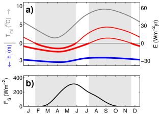
Figure 1: Sea ice seasonal cycle in a warming climate and solar radiation. (a) Seasonal cycle of stable solutions of the full nonlinear model are illustrated by plotting the model state $E$ (energy per unit area in ocean mixed layer sensible heat or sea ice latent heat) versus time of year. Four solutions are plotted, each with different levels of surface heating $\Delta F_{0}$: a perennial ice state (blue curve, $\Delta F_{0}=0$), seasonally ice-free states with most of the year ice-covered (lower red curve, $\Delta F_{0}=21$ Wm^-2) or most of the year ice-free (upper red curve, $\Delta F_{0}=23$ Wm^-2), and a perennially ice-free state (gray curve, $\Delta F_{0}=19$ Wm^-2). As described in equation (1), when $E>0$, it represents the mixed layer temperature of an ice-free ocean ($E=c_{ml}H_{ml}T_{ml}$). At $E=0$, the ocean mixed layer reaches the freezing point ($T_{ml}=0$^∘C), and further cooling will cause ice to grow. When $E<0$, it represents the sea ice thickness ($E=-L_{i}h_{i}$); note that ice thickness increases downward. Model solutions are drawn with thicker lines when the ocean is ice-covered and thinner lines when the ocean is ice-free. Solutions are obtained by integrating equations (2)-(4) with seasonally varying parameter values given in Table S1 (Supporting Information) until the model has converged on a steady-state seasonal cycle. The light gray shaded region to the right represents the first months to become ice-free in a warming climate (demarcated by zero-crossings of the seasonally ice-free solution with $\Delta F_{0}=21$ Wm^-2), while the light gray shaded region to the left represents the last months that are ice-covered in a further warmed climate (demarcated by zero-crossings of the seasonally ice-free solution with $\Delta F_{0}=23$ Wm^-2). (b) Seasonal cycle of incident solar radiation specified in the model based on central Arctic surface observations [13], indicating that the first months to become ice-free in a warming climate (light gray region to right) and the last months to be ice-covered in a further warmed climate (light gray region to left) experience similar amounts of solar radiation. Note that the radiation curve is asymmetric due to seasonal differences in Arctic cloudiness, but the qualitative results presented here do not depend on this asymmetry.

The annual minimum sea ice area and thickness is commonly referred to as “summer” sea ice and the annual maximum is commonly referred to as “winter” sea ice. This nomenclature may carry with it the implication that the ice-albedo feedback, which depends on the magnitude of the incident solar radiation, would be most prominent during the retreat of the summer sea ice cover. Indeed, it is often conjectured that a critical threshold for the loss of summer Arctic sea ice may be more likely than a threshold for the loss of winter ice [8]. However, as is illustrated by Fig. 1b, this terminology can be misleading because the ice cover receives a similar amount of incident solar radiation during the period of annual maximum as at annual minimum. The light gray shaded regions in Fig. 1 illustrate the key transition periods in the state of the Arctic Ocean during the transition from perennial ice cover to seasonally ice-free conditions (gray region to right) and from seasonally ice-free conditions to perennially ice-free conditions (gray region to left). Both of these periods experience roughly equivalent amounts of incident solar radiation (Fig. 1b), with somewhat more solar radiation occurring during the period associated with the loss of winter ice (light gray region to left). Hence the ice-albedo feedback should be expected to be similarly strong during a transition to perennially ice-free conditions in a very warm climate (i.e., loss of winter ice) as during a more imminent possible warming to seasonally ice-free conditions (i.e., loss of summer ice).

2.2 Bifurcation thresholds

Figure 2: Bifurcation diagram for the partially linearized model, where nonlinear sea ice thermodynamic effects have been excluded but the ice-albedo feedback has been retained (equations (2)-(3), (5)). For each value of the surface heating $\Delta F_{0}$, the model is integrated until it converges on a steady-state seasonal cycle, and the annual maximum (upper curve) and annual minimum (lower curve) values of $E$ are plotted. Solutions with perennial sea ice cover are indicated in blue, seasonally ice-free solutions in red, and perennially ice-free solutions in gray. Dashed lines indicate unstable solutions, which have been located by constructing an annual Poincaré map and finding the fixed points (i.e., numerically integrating the model for one year starting from an array of initial conditions and identifying the solutions with the same value of $E$ at the end of the year as the initial condition). The curves have been smoothed with a boxcar filter to suppress a small level of noise associated with numerical integration. Note that the lines are slightly curved at the two bifurcation points due to the smooth albedo transition associated with $h_{\alpha}>0$. The vertical axis is labeled as in Fig. 1a.

We begin the bifurcation analysis using the partially linearized version of the model (equations (2), (4)-(5)) to focus on the effect of albedo in the absence of other nonlinearities. In this representation, the Arctic Ocean is viewed as a simple radiating thermal reservoir with a temperature-dependent albedo, and the model exhibits a linear relaxation to a stable solution in each albedo regime. As would be expected by analogy with the discussion above of an annual mean Arctic Ocean with a variable sea ice edge, Fig. 2 illustrates that when $\Delta F_{0}$ becomes sufficiently large for the ocean to remain perennially ice-free with $\alpha=\alpha_{ml}$, an unstable seasonally ice-free solution (red dashed curve) appears in a saddle-node bifurcation of cycles (for a discussion of the theory of bifurcations in periodic systems, see, e.g., Strogatz [18]). The unstable solution separates stable solutions with perennial ice (blue curve) or perennially ice-free conditions (gray curve). The perennial ice regime collides with the unstable seasonally ice-free state and disappears in a second saddle-node bifurcation of cycles at the point where $\Delta F_{0}$ becomes sufficiently large that the ice completely melts at the time of annual maximum $E$ in the cold stable state. Due to there being significant incident solar radiation during both the maximum and minimum periods of the seasonal cycle of $E$ (Fig. 1), the ice-albedo feedback ensures that all seasonally ice-free solutions will be unstable (Fig. 2).

When nonlinear sea ice thermodynamic effects are included (equations (2)-(4)), basal ice formation is controlled by a diffusive vertical heat flux of $k_{i}\Delta T/h_{i}$, where $\Delta T$ is the difference between surface and basal temperatures and the base is assumed to be at the freezing point. This causes thin ice to grow significantly faster than thick ice [13]. It would also cause thin ice to experience greater basal ablation during the summer melt season, but the surface temperature only warms until it reaches the freezing point ($\Delta T=0$) and surface melt begins, making the rate of melt less sensitive to thickness. These two effects, both nonlinear in $E$, are expressed in equation (3) by the $-k_{i}/h=k_{i}L_{i}/E$ term in the denominator and the ramp function $\mathcal{R}(x)$, respectively. The result is an increase in the rate of growth for thin ice which is more stabilizing for thinner ice, as pointed out [19] and applied [20] in previous studies. This is in contrast to the state-independent linear mixed layer stabilizing term, $-F_{T}(t)E/c_{ml}H_{ml}$, which applies when $E>0$ (equations (2) and (3)).

These nonlinearities allow for the existence of a stable seasonally ice-free solution (Fig. 3). When a sufficiently large value of $\Delta F_{0}$ is chosen such that the cold solution becomes ice-free during a small part of the year, a slight increase in temperature would lead to a longer open-water period and a thinner seasonal ice cover. Although the increased period of open water promotes warming through the ice-albedo feedback, the thinner ice grows significantly faster because of the sea ice thermodynamic effects which are nonlinear in $E$. During the ice-covered portion of the year, the stability of the solution is controlled by this strong nonlinear stabilizing effect, but during the ice-free portion of the year it is replaced by the weaker linear mixed layer stabilizing term. This causes the stabilizing sea ice thermodynamic effects to dominate the destabilizing ice-albedo feedback and allow a stable seasonally ice-free solution only when there is ice cover during a sufficiently long portion of the year. Nonetheless, the ice-albedo feedback causes this regime to warm at an increased rate in response to increasing heat flux (compare slopes of red and blue curves in Fig. 3). As the ice-covered fraction of the year decreases in a warming climate, the stabilizing ice thermodynamic effects become less pronounced in the full annual cycle, and a bifurcation occurs when ice covers the Arctic Ocean during a sufficiently small fraction of the year to allow the ice-albedo feedback to dominate. Hence when the Arctic warms beyond this point, the system supports only an ice-free solution (Fig. 3).

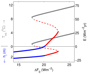
Figure 3: Bifurcation diagram for the full nonlinear model (equations (2)-(4)). Axes and colors are as described in the caption of Fig. 2. The inclusion of nonlinear sea ice thermodynamic effects stabilizes the model when sea ice is present during a sufficiently large fraction of the year, allowing stable seasonally ice-free solutions (red solid curves). Under a modest warming ($\Delta F_{0}=15$ Wm^-2), modeled sea ice thickness varies seasonally between 0.9m and 2.2m. Further warming ($\Delta F_{0}=20$ Wm^-2) causes the September ice cover to disappear, and the system undergoes a smooth transition to seasonally ice-free conditions. When the model is further warmed ($\Delta F_{0}=23$ Wm^-2), a saddle-node bifurcation occurs, and the wintertime sea ice-cover abruptly disappears in an irreversible process. While the specific values of $\Delta F_{0}$ at which the transitions occur are sensitive to parameter choices, the qualitative features of Fig. 3 are highly robust to changes in model parameter values (Supporting Information Fig. S4).

3 Discussion

3.1 Comparison with results of other models

The theoretical treatment presented here is constructed to facilitate simple conceptual interpretation, and to this end many processes have been neglected. Factors including possible sea ice–cloud feedbacks [21, 22, 23, 24], the dependence of sea ice surface albedo on snow and melt pond coverage [25, 26], ocean heat flux convergence feedbacks [6, 27], changes in wind-driven ice dynamics [7], and changes in ice rheology [28] in a thinning ice cover [29] could potentially lead to other bifurcation thresholds or smooth out the threshold investigated here, akin to the smoothing of a first order phase transition due to statistical fluctuations [33]. We are emboldened in our approach, however, because behavior consistent with the mechanism proposed here can be found in the previously published results of models with a broad range of complexities. (i) A “toy model” which is forced by a step function seasonal cycle produced no stable seasonally ice-free solution in the published parameter regime [30], but by a slight adjustment of the tunable model parameters one can find a stable seasonally ice-free solution which coexists with a stable perennially ice-free solution (Supporting Information Fig. S5), consistent with the findings presented here. (ii) In a variant of the model used in this study that is significantly more complex (representing the simultaneous evolution of fractional Arctic sea ice coverage, mean thickness, and surface temperature, as well as ocean mixed layer temperature), increasing the level of greenhouse gas forcing leads to a gradual transition to seasonally ice-free solutions followed by a bifurcation threshold during the transition to perennially ice-free conditions [31], as in Fig. 3. (iii) Turning to the most complex current climate models, about half the coupled atmosphere–ocean global climate models used for the most recent IPCC report [32] predict seasonally ice-free Arctic Ocean conditions by the end of the 21st century, and none predict perennially ice-free conditions by the end of the 21st century. However, perennially ice-free Arctic Ocean conditions occur in two of the model simulations after CO₂ quadrupling. Neither of the models exhibits an abrupt transition when the annual minimum (September) ice cover disappears, but after further warming one of the models abruptly loses its March ice cover when it becomes perennially ice-free [27]. The physical mechanism presented here may help explain this abrupt loss of simulated March ice while the simulated September ice receded gradually.

3.2 Conclusions

Our analysis suggests that a sea ice bifurcation threshold (or “tipping point”) caused by the ice-albedo feedback is not expected to occur in the transition from current perennial sea ice conditions to a seasonally ice-free Arctic Ocean, but that a bifurcation threshold associated with the sudden loss of the remaining seasonal ice cover may occur in response to further heating. These results may be interpreted by viewing the state of the Arctic Ocean as comprising a full seasonal cycle, which can include ice-covered periods as well as ice-free periods. The ice-albedo feedback promotes the existence of multiple states, allowing the possibility of abrupt transitions in the sea ice cover as the Arctic is gradually forced to warm. Because a similar amount of solar radiation is incident at the surface during the first months to become ice-free in a warming climate as during the final months to lose their ice in a further warmed climate, the ice-albedo feedback is similarly strong during both transitions. The asymmetry between these two transitions is associated with the fundamental nonlinearities of sea ice thermodynamic effects, which make the Arctic climate more stable when sea ice is present than when the open ocean is exposed. Hence when sea ice covers the Arctic Ocean during fewer months of the year, the state of the Arctic becomes less stable and more susceptible to destabilization by the ice-albedo feedback. In a warming climate, as discussed above, this causes irreversible threshold behavior during the potential distant loss of winter ice, but not during the more imminent possible loss of summer (September) ice.

The relevance of any basic theory to the actual future evolution of the complex climate system must be carefully qualified. Since the time scale associated with the sea ice response to a change in forcing may be decadal, and the time scale associated with increasing greenhouse gas concentrations may be similar, the system may not be operating close to a steady-state. In the gradual approach to steady-state under a continual change in forcing, the difference between a region of the steady-state solution with increased sensitivity to the forcing and an actual discontinuous bifurcation threshold (as in Fig. 3) could be difficult to discern. If greenhouse gas concentrations were reduced after crossing a bifurcation threshold, however, the possible irreversibility of the trajectory would certainly be expected to be relevant.

- [1] Stroeve, JC et al. (2005) Tracking the Arctic’s shrinking ice cover: Another extreme September minimum in 2004. Geophys Res Lett 32:L04501.
- [2] Perovich, DK et al. (2007) Increasing solar heating of the Arctic Ocean and adjacent seas, 1979-2005: Attribution and role in the ice-albedo feedback. Geophys Res Lett 34:L19505.
- [3] Lindsay, RW, Zhang, J (2005) The thinning of Arctic sea ice, 1988-2003: Have we passed a tipping point? J Clim 18:4879–4894.
- [4] Overpeck, J et al. (2005) Arctic system on trajectory to new, seasonally ice-free state. EOS 86:309–313.
- [5] Serreze, MC, Francis, JA (2006) The Arctic amplification debate. Clim Change 76:241–264.
- [6] Holland, MM, Bitz, CM, Tremblay, B (2006) Future abrupt reductions in the summer Arctic sea ice. Geophys Res Lett 33:L23503.
- [7] Maslanik, J et al. (2007) A younger, thinner arctic ice cover: Increased potential for rapid, extensive sea-ice loss. Geophys Res Lett 34:L24501.
- [8] Lenton, TM et al. (2008) Tipping elements in the Earth’s climate system. Proc Nat Acad Sci USA 105:1786–1793.
- [9] Merryfield, W, Holland, M, Monahan, A (2008) in Arctic Sea Ice Decline: Observations, Projections, Mechanisms, and Implications, eds Bitz, C, DeWeaver, E (Am Geophys Union), in press.
- [10] Budyko, MI (1969) The effect of solar radiation variations on the climate of the earth. Tellus 21:611–619.
- [11] Sellers, WD (1969) A global climate model based on the energy balance of the earth-atmosphere system. J Appl Meteor 8:392–400.
- [12] North, GR (1990) Multiple solutions in energy-balance climate models. Global Planet Change 82:225–235.
- [13] Maykut, GA, Untersteiner, N (1971) Some results from a time-dependent thermodynamic model of sea ice. J Geophys Res 76:1550–1575.
- [14] Maykut, GA, Church, PE (1973) Radiation climate of Barrow, Alaska, 1962-66. J Appl Meteor 12:620–628.
- [15] Kalnay, E et al. (1996) The NCEP/NCAR 40-year reanalysis project. Bull Amer Meteor Soc 77:437–471.
- [16] Nakamura, N, Oort, AH (1988) Atmospheric heat budgets of the polar-regions. J Geophys Res 93:9510–9524.
- [17] Kwok, R, Cunningham, GF, Pang, SS (2004) Fram strait sea ice outflow. J Geophys Res 109:C01009.
- [18] Strogatz, SH (1994) Nonlinear Dynamics and Chaos (Perseus Books).
- [19] Maykut, G (1986) in The geophysics of sea ice, ed Untersteiner, N (Plenium), pp 395–463.
- [20] Bitz, CM, Roe, GH (2004) A mechanism for the high rate of sea ice thinning in the arctic ocean. J Clim 17:3623–3632.
- [21] Kellogg, WW (1975) in Climate of the Arctic, eds Weller, G, Bowling, SA (Geophys Inst, Univ Alaska Fairbanks), pp 111–116.
- [22] Panel on Climate Change Feedbacks (2003) Understanding Climate Change Feedbacks (National Academies Press).
- [23] Vavrus, S (2004) The impact of cloud feedbacks on arctic climate under greenhouse forcing. J Clim 17:603–615.
- [24] Abbot, DS, Tziperman, E (2008) Winter Arctic sea ice uncertainty under global warming due to a cloud radiative feedback. Submitted to J Clim.
- [25] Curry, JA, Schramm, JL, Ebert, EE (1995) Sea-ice albedo climate feedback mechanism. J Clim 8:240–247.
- [26] Flato, GM, Brown, RD (1996) Variability and climate sensitivity of landfast Arctic sea ice. J Geophys Res 101:25767–25777.
- [27] Winton, M (2006) Does the arctic sea ice have a tipping point? Geophys Res Lett 33:L23504.
- [28] Zhang, JL, Rothrock, DA (2005) Effect of sea ice rheology in numerical investigations of climate. J Geophys Res 110: C08014.
- [29] Rothrock, DA, Percival, DB, Wensnahan, M (2008) The decline in Arctic sea-ice thickness: Separating the spatial, annual, and interannual variability in a quarter century of submarine data. J Geophys Res 113:C05003.
- [30] Thorndike, AS (1992) A toy model linking atmospheric thermal radiation and sea ice growth. J Geophys Res 97:9401–9410.
- [31] Eisenman, I (2007) in 2006 Program of Studies: Ice (Geophysical Fluid Dynamics Program) (Woods Hole Oceanog. Inst. Tech. Rept. 2007-02), pp 133–161 http://gfd.whoi.edu/page.do?pid=12938.
- [32] Solomon, S et al., eds (2007) Climate change 2007: The Physical Science Basis. Contribution of Working Group I to the Fourth Assessment Report of the Intergovernmental Panel on Climate Change (Cambridge University Press), p 996.
- [33] Lifshitz, EM, Pitaevskii, LP (1980) Statistical physics (Pergamon, Oxford).