The origin of ’Great Walls’

Abstract:

A new semi-analytical model that explains the formation and sizes of the ’great walls’ - the largest structures observed in the universe is suggested. Although the basis of the model is the Zel’dovich approximation it has been used in a new way very different from the previous studies. Instead of traditional approach that evaluates the nonlinear density field it has been utilized for identification of the regions in Lagrangian space that after the mapping to real or redshift space (depending on the kind of structure is studied) end up in the regions where shell-crossing occurs. The set of these regions in Lagrangian space form the progenitor of the structure and after the mapping it determines the pattern of the structure in real or redshift space. The particle trajectories have crossed in such regions and the mapping is no longer unique there. The progenitor after mapping makes only one stream in the multi-stream flow regions therefore it does not comprise all the mass. Nevertheless, it approximately retains the shape of the structure. The progenitor of the structure in real space is determined by the linear density field along with two non-Gaussian fields derived from the initial potential. Its shape in Eulerian space is also affected by the displacement field. The progenitor of the structure in redshift space also depends on these fields but in addition it is strongly affected by two anisotropic fields that determine the pattern of great walls as well as their huge sizes. All the fields used in the mappings are derived from the linear potential smoothed at the current scale of nonlinearity which is $R_{nl}=2.7$ h^-1Mpc for the adopted parameters of the $\Lambda$CDM universe normalized to $\sigma_{8}=0.8$. The model predicts the existence of walls with sizes significantly greater than 500 h^-1Mpc that may be found in sufficiently large redshift surveys.

1 Introduction

The first indications of the existence of superclusters of galaxies bridging the clusters of galaxies [1, 2] was confirmed by the CfA redshift survey [3]. In the following two decades the discovery of huge concentrations of galaxies spanning over 200 h^-1Mpc were reported (e.g., [4, 5]). They were dubbed ”great walls” due to their sizes and geometry in redshift space. The current record belongs to ”a Sloan Great Wall of galaxies 1.37 billion light years long, 80% longer than the Great Wall discovered by Geller and Huchra and therefore the largest observed structure in the universe” [5]. Taking into account that the SDSS redshift survey is much larger and deeper than CfA one may wonder whether the Sloan Great Wall will remain the greatest wall or even greater walls will be found in the future redshift surveys and if it is so how large it may be. The answer to this question may depend to certain extent on the exact definition of the walls. For instance, some definitions may result in the percolating system of filaments and walls that would span throughout the whole volume. However even in this case the essential constituents can be probably identified and measured. We show that by restricting the analysis to the issues of overall geometry and scale of the largest walls one can alleviate some of the problems of this kind and make some progress. In particular, the details of the density distribution within the walls, such as the accurate positions and masses of halos become less important if the scales of interest exceeds $\sim$10 h^-1Mpc.

We begin with a brief discussion of the structure in real space. The scale separating the nonlinear regime of the gravitational growth from linear or mildly nonlinear regimes is roughly around 5 h^-1Mpc which is close to the galaxy correlation scale. It seems to be by far too small to be directly relevant to the scale of filaments some of them are a least 70 – 100 h^-1Mpc long. Bond, Kofman and Pogosyan [6] (hereafter BKP) suggested that the filamentary network in real space with a typical scale of $\sim$30 h^-1Mpc can be explained by invoking the correlation bridges between relatively high and therefore rare peaks in the linear density field filtered on scales greater than $R_{\rm b}$ such that $\sigma_{\rho}(R_{\rm b})\lesssim 1$. Unfortunately, the BKP model has not provided a framework for a quantitative evaluation of the density contrast in the filaments bridging the clusters of galaxies from the enhancement of the conditional correlation function between two or more peaks. Besides, the gravitational growth of the structure in the universe is a deterministic process if the linear perturbation field is specified. Therefore, one may seek a deterministic relation between the initial field and the final structure at least in cosmological simulations where the full information is available. In addition, the cluster analysis of the nonlinear dark matter density field in real space obtained by N-body simulation in the $\Lambda$CDM model [7] revealed the filaments with lengths up to $\sim$100 h^-1Mpc [8] i.e., significantly greater than 30 h^-1Mpc. A similar analysis of the mock galaxy catalogs [9] demonstrated the presence of even longer filaments in redshift space, up to $\sim$ 150 h^-1Mpc [10]. Both numbers are almost certainly affected by the simulation box sizes (240 h^-1Mpc in the former and 346 h^-1Mpc in the latter case) and could be even longer in larger boxes. The simulated dark matter density fields and especially mock galaxy catalogs look similar to the observed distribution of galaxies as well as they have similar statistics of various kinds that makes the model viable. However, the emergence of the nonlinear structures (great walls) $\sim$ 50 – 100 times greater than the scale of nonlinearity remans unexplained even in the cosmological N-body simulations where the full information about the both initial conditions and formed structure is available.

It has been realized for a long time that the structures in real space and observed in redshift space have different pdfs, power spectra, correlation functions, and higher order moments (e.g., [11, 12, 13, 14, 15, 16]). The redshift-space correlation function has an oblate shape on scales greater than a few h^-1Mpc indicating the presence of anisotropic structures in redshift space flattened in the radial direction. However, the measurements do not go beyond $\sim$ 30 h^-1Mpc where the correlation function drops to $\sim 0.1$ and the signal drowns in noise [16]. Theory has not made any specific predictions concerning the structure in the universe on scales greater than 100 h^-1Mpc therefore the conventional wisdom is that the perturbations on such scales must be in the linear regime.

The ’finger of God’ is the most conspicuous and best understood effect in redshift space. However, it is a relatively small scale effect and cannot explain the coherence of the great walls over a few hundred h^-1Mpc. It has been also demonstrated in [17, 18] that the size of the structures in the redshift space is considerably greater than that of the parent structures in real space. In addition, the authors emphasized a characteristic circular pattern in redshift space and the increased spacing between the structures in the redshift direction. However, they neither mentioned the enlargement of sizes of the structures in the transverse direction nor provided explanation to their observations.

The presence of walls up to 150 h^-1Mpc in length in redshift space in three-dimensional simulations based on the adhesion approximation was emphasized in [19]. The authors pointed out that the correlation function was weak or even negative at these scales. They also observed that $\sim$ 100 h^-1Mpc walls grow from several favorably aligned high-density peaks in the linear density field, each coherent over $\sim$ 20 h^-1Mpc. This seems to be a factual description of the process, however similarly to the BKP model it requires a dynamical model different from the linear theory of gravitational instability. The major problem with the structures spanning over $\sim$ 300 h^-1Mpc arises from a lack of a natural scale of this magnitude in the linear density field. If the field is smoothed with say 100 h^-1Mpc or greater scale than its amplitude becomes so low that such a field would remain almost perfectly linear at the present time.

We view the formation of the structure as a continuous mapping from the initial practically uniform state in Lagrangian space to the final highly inhomogeneous and anisotropic distribution of mass on scales up to $\sim$ 100 h^-1Mpc in Eulerian space followed by another mapping to redshift space where the largest structures become greater than 300 h^-1Mpc. These mappings involve the transport of mass (although not physical in the case of the mapping to redshift space), however the rms displacement of mass elements is only about 15 h^-1Mpc and therefore it cannot produce the structures of needed sizes by itself. Thus, the certain initial fields i.e., the fields present in the linear stage and playing an important role in the nonlinear dynamics must have scales in the range of 100 h^-1Mpc or even greater. The major goal of this paper is to show that the fields having needed properties exist in Lagrangian space. The outcome of their combined effect is the definition of two parent structures that are the progenitors of the large-scale structures: one in real and the other in redshift space. Being closely related two progenitors are still quite distinct. The properties of the progenitors are determined by a combination of Gaussian and non-Gaussian fields derived from the initial gravitational potential smoothed with a Gaussian filter at the scale of nonlinearity $R_{\rm nl}$ defined by the equation $<\delta^{2}_{\rm lin}(R_{\rm nl})>=1$, where $\delta\equiv\delta\rho/\bar{\rho}$. In the standard $\Lambda$CDM model normalized to $\sigma_{8}\approx 0.8$ this scale is $R_{\rm nl}$ = 2.7 h^-1Mpc. The choice of the filter and filtering scale for 2D illustrations approximately corresponds to an optimal choice of the filter and scale in 3D simulations that studied the accuracy of the Truncated Zel’dovich Approximation (TZA) in a set of power law models in the Einstinen-de Sitter model [22]. Some adjustment will be probably needed for the $\Lambda$CDM model in 3D. Based on that study I would conservatively guess that the change in $R_{\rm nl}$ would not be greater than 30%. No fields smoothed at greater scales are involved in the mapping. The structure resulting from the mapping of the progenitors cannot and is not supposed to reproduce accurately the mass or galaxy number densities, however the overall shape and sizes of the structure in real space and great walls in redshift space must be depicted quite well.

We use TZA as a mapping device for both mapping [20, 22, 21, 15]. In this paper we will concentrate on the lengths of the progenitors in the Lagrangian space and their transformation caused by the mapping to Eulerian and redshift space.

We illustrate the model by two-dimensional plots. Although no two-dimensional model can reproduce all the properties of a three-dimensional system it may provide a reasonably good description of major ideas. In order to make the appearance of illustrations more realistic we use the linear power spectrum $P^{2D}(k)=k\,P^{3D}(k)$, where $P^{3D}(k)$ is the power spectrum of the linear density perturbations in the $\Lambda$CDM model with parameters $h=0.7$, $\Omega_{m}=0.3$, $\Omega_{b}=0.047$, $n=1$. We use the BBKS transfer function [23] with the $\Gamma$-parameter given by [24]. This choice of two-dimensional power spectrum retains all the moments $<k^{j}>$ of the three-dimensional spectrum and therefore all the scales of the two-dimensional field determined by the ratio of two moments (e.g., the scale of peaks $R_{*}^{2}\sim<k^{2}>/<k^{4}>$) remain similar to that of the three-dimensional field except a small factor $\sqrt{3/2}=1.2$. The two-dimensional fields were generated in 1024 h^-1Mpc box on 1024² mesh.

The rest of the paper is organized as follows. Section 2 outlines the dynamical model and fields involved in both mappings. Section 3 provides two dimensional illustrations that elucidate the main concepts of the model, the axes in the figures showing various fields are given in h^-1Mpc. Section 4 discuss the differences between 2D and 3D cases, Sec. 5 summarizes the results and outline the further problems, finally the appendix gives the joint density probability function of three invariants of the deformation tensor that are used in the mappings.

2 Model

The dominant feature of the process of the structure formation is usually dubbed as the hierarchical clustering. It simply means that small halos generally form earlier than the larger ones. Thus, more massive halos are formed by consecutive merging of smaller halos. The merging process effectively stops on the scale of $R_{\rm nl}$ or on a little greater scale. It is a well established fact that he formation of the structures on larger scales is mainly determined by the long wave part of the initial spectrum with $k<R^{-1}_{\rm nl}$ [25]. [25] also pointed out that the changes in the high-frequency ($k>R^{-1}_{\rm nl}$) components of the initial conditions did not affect much the evolution of long waves. A direct comparison of the nonlinear density fields obtained in the N-body simulations of models with and without high-frequency components (Truncated Zel’dovich Approximation) in the initial conditions has also shown a very good agreement [20, 22, 21]. In general, the Zel’dovich approximation ”gives a reasonable description of the overall pattern of N-body simulations” [6].

Using the comoving coordinates $\vec{x}\equiv{\bf r}/a(t)$ where $a(t)$ is the scale factor describing the uniform expansion of the universe the Zel’dovich approximation [26] (see also [27]) becomes

$$x_{i}({\bf q},t)=q_{i}+D(t)s_{i}({\bf q}),$$ (1)

where vector ${\bf q}$ gives the Lagrangian (initial) position of a fluid element, ${\bf x}$ is the Eulireian position of the fluid element at time $t$, $D(t)$ describes the linear growing mode of fluctuations, $s_{i}({\bf q})=-\partial\Phi/\partial q_{i}$ is the displacement field and $\Phi({\bf q})$ is the linear gravitational potential field. Thus, our dynamical model is the Zel’dovich approximation applied to the initial fluctuation field smoothed over the nonlinear scale $R_{\rm nl}$ which equals 2.7 h^-1Mpc in the $\Lambda$CDM model normalized to $\sigma_{8}=0.8$.

Instead of traditional approach that tries to evaluate the evolution of density field we suggest to consider its inverse i.e., the evolution of specific volume $V=\rho^{-1}$. The specific volume is more suitable quantity for our purpose because it allows an easy separation of the effects related to various fields. We would like to remind that we do not use this model for accurate predicting of the nonlinear density field but only for approximate identification of high density regions. The specific volume is given by the Jacobian

$${V_{x}({\bf q},t)\over<{V}>}=J_{x}=\det\left({\partial x_{i}\over\partial q_{j}}\right).$$ (2)

The growth of density corresponds to the decrease of the specific volume. Some fluid elements may collapse to zero volume and at later time their volumes predicted by eq. 2 become even negative however this is an easy problem. Negativeness of the density or specific volume simply reflects the fact that such a fluid element turns inside out and the positiveness of the density can be easily restored by taking the absolute value of the Jacobian. It also indicates that the trajectories of fluid elements are crossed and the mapping in no longer unique. This creates a much more serious problem that does not have a simple solution even in the frame of the Zel’dovich approximation (apart from breaking the approximation within the regions where shell-crossing occurs) mainly because the problem becomes nonlocal. The set of fluid elements that collapse by the present time form a structure in Lagrangian space, we shall call it the progenitor or parent structure. The parent structure mapped to Eulerian space by means of eq. 1 forms the pattern of the large-scale structure. It is worth stressing that the parent elements do not represent the total mass contained in the large-scale structure however they approximately mark the regions of highest density. The situation becomes more complex if we recall that the large-scale structure forms from highly nonuniform state where practically all the mass is already in the form of virialized halos. However, as the previous studies showed ( e.g.,[27, 25, 20, 22, 21]) the overall distribution of the halo number density corresponds to this model quite well.

The Jacobian can be expressed in terms of the invariants ($I_{1},I_{2},I_{3}$) or eigen values ($\lambda_{1},\lambda_{2},\lambda_{3}$) of the deformation tensor $d_{ij}=-\partial s_{i}/\partial q_{j}=\partial^{2}\Phi/\partial q_{i}\partial q_{j}$

$$J_{x}({\bf q},t) = 1-D(t)I_{1}({\bf q})+D^{2}(t)I_{2}({\bf q})-D^{3}(t)I_{3}({\bf q})$$ (3)

$$= \left[1-D(t)\lambda_{1}({\bf q})][1-D(t)\lambda_{2}({\bf q})][1-D(t)\lambda_{3}({\bf q})\right],$$

where

$$I_{1}=d_{11}+d_{22}+d_{33},~{}~{}I_{2}=M_{11}+M_{22}+M_{33},~{}~{}I_{3}=\left|\begin{array}[]{c c c}d_{11}&d_{12}&d_{13}\\ d_{12}&d_{22}&d_{23}\\ d_{13}&d_{23}&d_{33}\end{array}\right|,$$ (4)

and $M_{ij}$ are the minors of the corresponding elements of the determinant $I_{3}$. The eigen values are the solutions of the characteristic equation

$$\lambda^{3}-I_{1}\lambda^{2}+I_{2}\lambda-I_{3}=0.$$ (5)

It always has three real solutions because the mapping is generated by the potential vector field $s_{i}({\bf q})$ and therefore the deformation tensor is symmetric $d_{ij}=d_{ji}=\partial^{2}\Phi/\partial q_{i}\partial q_{j}$; it is convenient to assume the solutions to be ordered at every point $\lambda_{1}({\bf q})\geq\lambda_{2}({\bf q})$ and $\lambda_{2}({\bf q})\geq\lambda_{3}({\bf q})$.

Equation $J_{x}({\bf q},t)=0$ has obviously three solutions for $D$ as well: $D_{i}=1/\lambda_{i}$. If any of them lies in the interval $0<D_{i}({\bf q})<1$ we consider the fluid element with Lagrangian coordinates ${\bf q}$ to belong the progenitor of the structure. Condition $0<\lambda_{1}({\bf q})<1$ is equivalent to the above condition for $D_{i}({\bf q})$ but it is less general and cannot be used for the mapping to redshift space where it is not of potential type.

In order to describe the mapping to redshift space ($\zeta_{i}$) we supplement eq. 1 with additional term (see e.g., [15])

$$\zeta_{i}=x_{i}+fDs_{k}({\bf q})n_{k}({\bf x})n_{i}({\bf x})=q_{i}+Ds_{i}({\bf q})+fDs_{k}({\bf q})n_{k}({\bf x})n_{i}({\bf x})$$ (6)

where ${\bf x}$ is given by eq. 1, $f=d\log D/d\log a\approx\Omega_{m}^{0.6}$ for the present time [11] or a better approximation given in [28]. The unit vector $n_{i}\equiv x_{i}/x$ is directed along the line of sight. We assume summation over repeated indices throughout the paper. The peculiar velocity $v^{(p)}_{i}=\dot{a}fDs_{i}$ and therefore the displacement of a galaxy from comoving Eulerian position, $x_{i}$ to redshift space position, $\zeta_{i}$, is $v^{(p)}_{k}n_{k}/(aH)=fDs_{k}n_{k}$ along the line of sight. The distances in Lagrangian, comoving Eulerian and redshift space are measured in h^-1Mpc.

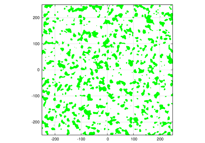
Figure 1: Lagrangian space. Regions $\delta({\bf q})>1$ or equvalently $1-I_{1}({\bf q})<0$ are shown in green.

The specific volume is equal to the corresponding Jacobian

$${V_{\zeta}({\bf q},t)\over<{V}>}=J_{\zeta}=\det\left({\partial\zeta_{i}\over\partial q_{j}}\right).$$ (7)

The evaluation of $V_{\zeta}$ in terms of the initial fields is a quite laborious task. Fortunately it allows a considerable simplification in the limit of $|D{\bf s}|\ll q$. Physically it means that the results are not reliable within 50 h^-1Mpc or so from the center but it is not very important since we are interested in much greater scales. The components of the Jacobian become (to the zeroth order in $|D{\bf s}|/q$)

$${\partial\zeta_{i}\over\partial q_{j}}\approx\delta_{ij}-D(d_{ij}+f\tilde{n}_{i}\tilde{n}_{k}d_{jk}),$$ (8)

where $\tilde{{\bf n}}={\bf q}/q$. Mapping to redshift space is neither irrotational nor solenodial which means that Jacobian $J_{\zeta}$ has no symmetry. Similarly to the Jacobian of the mapping to Eulerian space the determinant $J_{\zeta}$ can be expressed in terms of the invariants of the initial fields and the radial components of two tensors $d_{qq}$ and $M_{qq}$

$$J_{\zeta} = 1-DI_{1}+D^{2}(1+f)I_{2}-D^{3}(1+f)I_{3}-fDd_{qq}-fD^{2}M_{qq},$$ (9)

where $d_{qq}=\tilde{n}_{i}\tilde{n}_{j}d_{ij}$ and $M_{qq}=\tilde{n}_{i}\tilde{n}_{j}M_{ij}$ are the radial components of the deformation tensor and tensor made of the minors of the determinant $I_{3}$. The invariants are statistically isotropic fields although two of them ($I_{2}({\bf q})$ and $I_{3}({\bf q})$) are non-Gaussian. The last two terms depend on highly anisotropic fields: one $d_{qq}({\bf q})$ is Gaussian and the other $M_{qq}({\bf q})$ is non-Gaussian.

3 Two-dimensional illustration

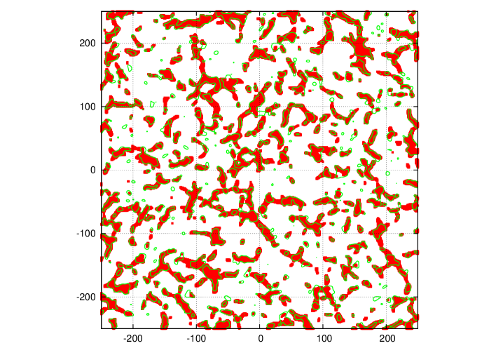
Figure 2: Lagrangian space. Red regions $1-I_{1}({\bf q})+I_{2}({\bf q})<0$, green contours $\delta({\bf q})=1$ correspond to the boundaries of the regions in fig. 1.

Major although not all features of the model can be illustrated by a two-dimensional model. Although the main goal of the paper is a study of the mapping to redshift space we briefly discuss the mapping to real space and show the importance of non-Gaussian fields for building the large-scale structure. We shall use a convenient normalization of function $D(t)$ such that at the present time $D(t_{0})=1$ and the variance of the linear density contrast field $\sigma^{2}_{\delta}=1$, parameter $f\approx 0.8$ for the chosen cosmological model.

3.1 Mapping to real space

The Jacobian of the mapping to Eulerian space in two dimensions depends on two statistically isotropic and homogeneous fields: one Gaussian $I_{1}({\bf q})$ and one non-Gaussian $I_{2}({\bf q})$

$${V_{x}\over<{V}>}=J_{x}=1-DI_{1}+D^{2}I_{2}.$$ (10)

The initial density contrast field $\delta_{in}\equiv\delta\rho/\bar{\rho}=D(t_{in})I_{1}$ is assumed to be Gaussian. Let us begin with the linear approximation ${V_{x}/<{V}>}=1-DI_{1}$. Linear theory formally predicts that the peaks with $\delta\geq 1$ shrink to the regions having formally negative volumes (and therefore negative density) by the present time. Figure 1 shows an example of the progenitor of the structure in Lagrangian space predicted by the linear theory ${V_{x}(t_{0},q)/<{V}>}=1-D(t_{0})I_{1}(q)=1-I_{1}(q)<0$. Although the initial power spectrum is filtered with Gaussian windows $\exp(-k^{2}R_{f}^{2}/2)$ with $R_{f}=2.7$ h^-1Mpc some peaks $\delta>1$ have quite large lengths reaching $\sim 30$ h^-1Mpc.

The full nonlinear model $v_{x}(t_{0},q)=1-D(t_{0})I_{1}(q)+D^{2}(t_{0})I_{2}(q)=1-I_{1}(q)+I_{2}(q)<0$ predicts the progenitor of the structure shown in Figure 2 in red. The green contours show the boundaries of the linear progenitor shown in fig.1, thus one can see both the similarities and differences of two fields. In order to make an eye ball estimate of sizes easier we plot the grid on the background. The similarity of two fields is obvious but it is not unexpected because both fields depend on $I_{1}(q)$ and therefore strongly correlated. The effect of non-Gaussian $I_{2}$-field is quite remarkable. The red non-Gaussian regions are considerably longer than the linear density peaks. They also typically comprise several green regions therefore non-Gaussian field $I_{2}$ provides ”bridges” linking the peaks of linear density contrast field. This is in a good qualitative agreement with the observations made by Weinberg and Gunn [19] who emphasized that the large structures usually consist of several peaks in the linear density field. There is also no contradiction to the role of the correlation between linear density peaks in the BKP model [6], although the the higher peaks of the field smoothed with greater scale is assumed in the BKP model.

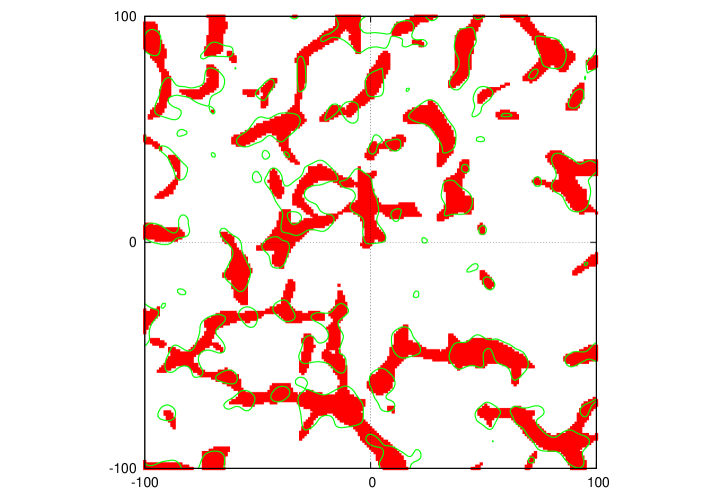
Figure 3: Lagrangian space, the central 200 h^-1Mpc box of fig.2. Red regions $1-I_{1}({\bf q})+I_{2}({\bf q})<0$, green contours $\delta({\bf q})=1$ correspond to the boundaries of the regions in fig.1.

The green contours totally comprise 15.9% of the area. It is remarkable that the red regions where the nonlinear condition $1-I_{1}(q)+I_{2}(q)<0$ is satisfied occupy slightly less area (15.3% ) than the green contours. Despite the greater lengths of the nonlinear progenitor reaching over 100 h^-1Mpc red regions are generally slimmer than their counterparts in the linear progenitor. The resolution of fig.2 is far too low to reveal this completely. However, it is obvious in fig.3 where the central part of fig.2 is zoomed in. In addition, small isolated regions of the linear progenitor disappear from the nonlinear one (empty green contours).

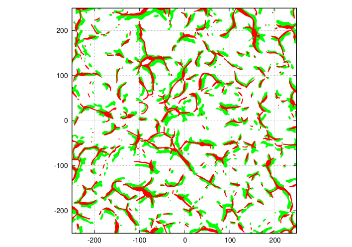
Figure 4: Eulerian space. The large-scale structure in Eulerian space (red) and the progenitor of the structure in Lagrangian space (green).

Figure 4 shows the structure in Eulerian space (red) along with the progenitor in Lagrangian space (green). The mapping makes the structure considerably slimmer than its progenitor in Lagrangian space although it is probably thicker than in reality [27]. Two points are worth stressing. First, neither lengths of the filaments no topology visibly change due to mapping itself. And second, the filaments do not move much, however those that moved were are displaced mostly in the transverse direction while the longitudinal displacement is significantly smaller. It is also worth recalling that the r.m.s. displacement of fluid elements from the Lagrangian to Eulerian positions is about 15 h^-1Mpc which greater than the thickness of the filaments but considerably smaller than their lengths. The mapping to real space also involves statistically isotropic Gaussian vector field $s_{i}({\bf q})=-\partial\Phi/\partial q_{i}$.

3.2 Mapping to redshift space

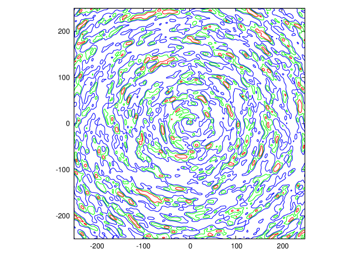
Figure 5: Lagrangian space. Contours $fd_{qq}({\bf q})=0.25,0.5,1$ are shown in blue, green and red respectively.

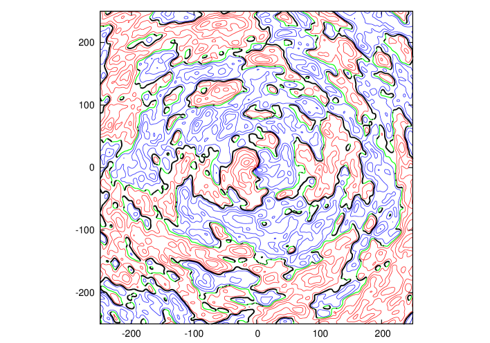
Figure 6: Lagrangian space. Contours of $fv_{q}({\bf q})>0$ are shown in red, $fv_{q}({\bf q})=0$ in green and $fv_{q}({\bf q})<0$ in blue. The segments of convergence i.e., the parts of the contour $v_{q}({\bf q})=0$ satisfying the condition $\partial v_{q}/\partial q<0$ are marked by black dots.

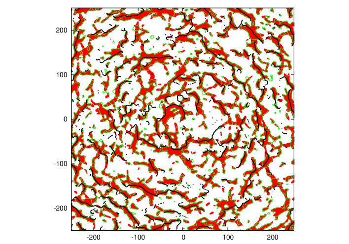
Figure 7: Lagrangian space. The nonlinear progenitor of the structure in redshift space defined by the condition eq. 11 is shown in red. Green contours show the regions defined by the linear condition $\delta({\bf q})\geq 1$. Black dots mark the segments of convergence.

We obtain the Jacobian of the mapping to redshift space in two dimensions from eq. 9

$$J_{\zeta}({\bf q},t)=1-DI_{1}+D^{2}(1+f)I_{2}-fDd_{qq},$$ (11)

where $I_{1}=d_{11}+d_{22}$ and $I_{2}=d_{11}d_{22}-d_{12}^{2}$ are the invariants of the deformation tensor in two dimensions, $d_{qq}=\tilde{n}_{1}^{2}d_{11}+2\tilde{n}_{1}\tilde{n}_{2}d_{12}+\tilde{n}_{2}^{2}d_{22}$ is the radial component of the deformation tensor. Compared to the mapping to Eulerian space the term proportional to $I_{2}$ is boosted by factor $1+f$. The Jacobian contains a highly anisotropic field $d_{qq}({\bf q})$ in the sense that the contours are significantly longer in the transverse direction than in radial direction as a result the field acquires a characteristic circular pattern (fig.5). The cause of this anisotropy becomes much more obvious if one considers the small angle approximation [12]. Now, let us consider the direction corresponding to $q_{1}$-axis. In this case $\tilde{{\bf n}}=(1,0)$ therefore $d_{qq}=d_{11}(q)=\partial^{2}\Phi({\bf q})/\partial q_{1}^{2}$. Differentiating potential two times with respect to $q_{1}$ multiplies the power spectrum by $k_{1}^{4}$ ($P_{d_{11}}({\bf k})=k_{1}^{4}P_{\Phi}(k)$) that effectively reduces the characteristic scale of the resulting field along $q_{1}$ direction while the scale along $q_{2}$ changes much less. In the case of arbitrary direction the reduction of the scale along radial direction is much stronger than in the transverse direction that generates a distinct circular pattern.

The mapping to redshift space also involves the radial component of the velocity field $v_{q}({\bf q})=fDs_{q}({\bf q})=-fD\partial\Phi/\partial q$ shown in fig.6. Although the vector field ${\bf s}({\bf q})$ itself is isotropic its components are highly anisotropic fields. Again, let us consider the small angle approximation and $v_{1}({\bf q})\propto s_{1}({\bf q})$ component of the velocity vector field. The power spectrum $P_{s_{1}}({\bf k})=k_{1}^{2}P_{\Phi}(k)$ is anisotropic with considerably more power along $k_{1}$ direction. Therefore the field $s_{1}({\bf q})$ has much smaller scale along $q_{1}$ direction than along $q_{2}$ direction. For an arbitrary direction $\tilde{n}_{i}=q_{i}/q$ it is translated into considerable anisotropies between radial and transverse directions. A natural expectation suggests that the structure in redshift space is shifted to the segments of the zero contour $v_{q}({\bf q})=0$ satisfying the convergence condition $\partial v_{q}/\partial q<0$ marked by black dots on green contour in fig.6. On the inner side of these segments the radial component of the peculiar velocity is positive and therefore directed away from the center while on the outer side it is negative and thus directed toward the center resulting in shifting mass to these lines by the mapping to redshift space.

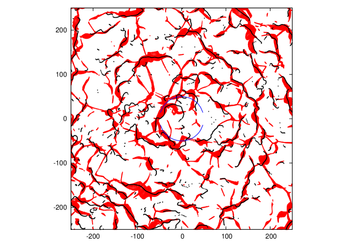
Figure 8: Redshift space. The large-scale structure is shown in red. The black lines are the parts of the contour $v_{q}({\bf q})\equiv v_{i}({\bf q})\tilde{n}_{i}({\bf q})=0$ selected by the condition $\partial v_{q}/\partial q<0$. Two blue arcs mark the central 50 h^-1Mpc region where the adopted approximation ($D|{\bf s}|/q\ll 1$ ) is not very accurate.

The progenitor of the structure in redshift space determined by eq. 11 is shown as red regions in fig.7. The green contours show the boundaries of the regions $\delta({\bf q})>1$ shown in fig.1 as green regions and also as green contours in fig.2. It is worth comparing the progenitors of the mappings to Eulerian (fig.2) and redshift space (fig.7). The circular pattern due to $fDd_{qq}$ term in eq. 11 is quite obvious in fig.7 but it is significantly less conspicuous than in fig.5 because the other two fields ($I_{1}$ and $I_{2}$) affecting the Jacobian are both statistically isotropic and homogeneous. The black dots mark the lines of convergence defined above and shown in fig.6. The convergence lines obviously correlate with the progenitor of the mapping to redshift space although the correlation is not perfect.

The result of the mapping of the nonlinear progenitor (eq. 11) to redshift space is shown as red regions in fig.8. If the linear progenitor was mapped to redshift space it would sit perfectly on top of the nonlinear structure, however it would remain significantly less connected than the nonlinear structure as the mapping is continuous. The figure illustrates a substantial change in the geometry caused by the mapping itself. The sizes of red filaments and voids between them are noticeably greater in redshift space than in Lagrangian space. Some smaller regions seen in Lagrangian space have merged into larger structures when mapped to redshift space. The difference between the structures in Eulerian (fig.4) and redshift space (fig.8) is quite substantial.

Figure 8 also shows the convergence segments of the zero line of the radial velocity field demonstrated in fig.6. Similarly to fig.7 the black dots are noticeably more numerous in red regions than between them. In this case the correlation is not entirely perfect either but it is quite obvious despite the fact that the black dots are plotted in Lagrangian space while the red structure is plotted in redshift space. As we have seen in fig.4 the mapping to Eulerian space does not shift the progenitor much and the following mapping to redshift space does not move the points with $v_{q}=0$. In a few cases the separate segments of the convergence set seem to be aligned forming the filaments with total length of over 500 h^-1Mpc. An example of this is the system of five segments that begins at distance about 200 h^-1Mpc toward 1h from the center and continues clockwise down to distance $\sim$150 h^-1Mpc toward 4h from the center.

The correlation between the structure in redshift space and the segments of convergence allows to use the lengths of the segment of convergence as predictors of the length of filaments. Figure 9 shows the segments of convergence i.e., the parts of line $v_{q}({\bf q})=0$ where additional conditions $\partial v_{q}/\partial q_{q}<0$ is satisfied. These lines are attractors of the nonlinear structure in redshift space. Inspecting the figure one can easily identify the lines extended over 500 h^-1Mpc that suggests the existence of the filaments of similar sizes. The field $s_{q}({\bf q})$ is closely related to the initial potential since $s_{q}({\bf q})=-\partial\Phi/\partial q$ and therefore may be affected by an insufficient size of the box. Thus, the actual size of largest walls can be even greater than suggested by fig.9 in real universe. The full three-dimensional N-body simulations checking this prediction are currently on the way.

Figure 9: Lagrangian space (1024 h^-1Mpc box). The black dots mark the segments of convergence i.e., the segments of contour $v_{q}({\bf q})=0$ where additional condition $\partial v_{q}/\partial q_{q}<0$ is satisfied. These lines are a kind of attractor of the structure in redshift space and their lengths are similar to the lengths of walls.

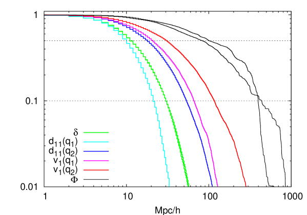
Figure 10: Cumulative probability function of the zero-crossing distances along two axes $q_{1}$ and $q_{2}$. The top doted line marks the median values of the probability functions.

3.3 Scales of Gaussian random fields

In cosmology Gaussian fields are often characterized by several scales derived from moments $<k^{2j}>\equiv(2\pi^{2})^{-1}\int k^{2j}P(k)k^{2}dkk^{2j}$ of the power spectrum $P(k)$ (e.g., [23]). The ratios of these moments generate a set of scales $R_{j}^{2}=3<k^{2j}>/<k^{2(j+1)}>$. Two particular scales $R_{1}\equiv R_{*}$ (using notation of ref. [23]) and $R_{0}$ are used the most often as the characteristics of linear density fields. The former is associated with the spatial distribution of peaks and is discussed in detail in [23]. The latter is referred to as the mean distance between crossing points of zero level [30]. [31] introduced the integral length scale $L=\xi^{-1}(0)\int_{0}^{\infty}\xi(r)dr=(\pi/2)\int_{0}^{\infty}kP(k)dk/\int_{0}^{\infty}k^{2}P(k)dk$, the physical meaning of which is not quite obvious. An example of using other scales in cosmology is given in [32]. The suggested model deals with the components of the deformation tensor $d_{ij}({\bf q})$ and displacement $s_{i}({\bf q})$ that are combined into radial components $d_{qq}({\bf q})$ and $s_{q}({\bf q})$. Here we consider the small angle approximation that fully described by $d_{11}$ and $s_{1}$ fields. The scales can be characterized by the distribution of distances between successive zeros of a field along two axes (see e.g., [18]). Figure 10 shows the cumulative probability functions of zero crossing distances for four fields ($\delta=I_{1},d_{11}$, $v_{1}$ and $\Phi$) along two axes ($q_{1}$ and $q_{2}$). The density contrast field is isotropic and both cpfs are practically identical. The potential field also must be statistically isotropic but it depends strongly on long wave part of the power spectrum. In fact the variance $\sigma^{2}_{\Phi}$ formally logarithmically diverges at $k\rightarrow 0$. However, this is not a serious physical problem. Heavens [33] pointed out that in a fixed sample volume (e.g.,the observable universe) the potential is well behaved, however we cannot determine the global zero level of the potential. He showed that by introducing $\Delta\Phi({\bf x})=\Phi({\bf x})-\Phi_{0}$, where $\Phi_{0}$ is the value of the potential at the observer location, the problems related to the divergence of $\sigma^{2}_{\Phi}$ are reduced to a weak dependence of the results on unknown value of $\Phi_{0}$. Such fields are known as locally homogeneous and locally isotopic fields and are discussed in Sec. 13 of ref. [31]. This dependence of the potential on the long wave part of the spectrum explains huge variations in the tail of the cumulative function seen in fig.10 (black solid lines). The scales along $q_{2}$ are much greater than along $q_{1}$ for both anisotropic fields $d_{11}$ and $v_{1}$. The level lines of all fields are quite wiggly therefore there are quite a few short distances between crossing points. The overall sizes are probably better characterized by the tails of the distributions. Here are the median and the value marking the top 10% distances along $q_{1}$ and $q_{2}$ axes for four fields in h^-1Mpc: median $\delta$(11, 11), $d_{11}$ (10, 18), $s_{1}$ (21, 31) and $\Phi$ (102, 84), top 10% $\delta$ (30, 30), $d_{11}$ (21, 54), $s_{1}$ (66, 117) and $\Phi$ (397, 437).

4 Implications for three-dimensional universe

The progenitor of the mapping to Eulerian space is determined by the interplay of three fields: one Gaussian $\delta=I_{1}$ and two non-Gaussian $I_{2}$ and $I_{3}$. It is easy to show that they do not correlate by the direct calculation of the corresponding integrals over the joint pdf (see Appendix). However the fact that two fields are non-Gaussian does not allow to declare them statistically independent and it makes the further analysis more challenging.

Many features of two-dimensional model although not all are expected to be very similar in three dimensions. Nonlinear term proportional to $I_{2}$ helps to fill the gaps between peaks of linear field $\delta=I_{1}({\bf q})>1$ in 2D and therefore boosts the length of filaments in Lagrangian space up to 70 –100 h^-1Mpc. There is no reason to doubt that it works in a similar way in 3D. In addition, the term proportional $I_{3}$ in eq. 3 is likely to boost the lengths of filaments even more. However, the further study is obviously needed both analytical and numerical.

The mapping to Eulerian space itself does not change significantly the lengths of the filaments and does not displace them much from the initial positions in 2D. The mapping in 3D is expected to be similar in this respect.

However, the mapping to redshift space differs in 3D significantly in a few respects. All three fields $d_{qq}$, $M_{qq}$ (see eq. 9) and $s_{q}$ (see eq. 6) have scales in the radial direction much shorter than in two transverse directions. This causes the progenitor and the structure in redshift space to acquire a circular pattern in 2D while it gives rise to the origin of shell like walls in 3D. The walls in redshift space expected to be neither homogeneous no thin but their transverse sizes must be considerably greater than the radial thickness. Similarly to the two-dimensional case the greatness of ’great walls’ comes from anisotropy of two Gaussian fields $d_{qq}$ and $s_{q}$ and in addition one non-Gaussian field, $M_{qq}$ derived from initial Gaussian field. As fig. 10 indicates the transverse coherence of both $d_{11}$ and especially $s_{1}$ field can easily exceed 100 h^-1Mpc. Two isotropic non-Gaussian fields $I_{2}$ and $I_{3}$ also contribute to the formation of the structure in redshift space since the corresponding terms are boosted by factor $1+f$ in the Jacobian $J_{\zeta}$ (eq. 9).

The convergence lines defined in 2D become the convergence surfaces in 3D, they are expected to provide a reasonable estimate of the transverse sizes of great walls.

5 Summary and discussion

We propose a new theoretical model that describes the formation of the large-scale structure in redshift space. It naturally explains the sizes of the observed great walls and predicts that even greater walls will be discovered in future deeper and larger redshift surveys. Although based on the Zel’dovich approximation [26] the suggested model uses it in a new and very different way. Instead of traditional approaches that focused on the evaluation of density or positions and velocities of the particles we introduce the notion of the progenitor of the large-scale structure. It is defined as a set of regions in Lagrangian space that after mapping to Eulerian or redshift space (depending on the kind of mapping we study) end up in the regions where the particle trajectories have crossed and the mapping is no longer unique. Neglecting the thermal velocities and assuming smooth initial condition the boundaries of these regions in Eulerian or redshift space are caustics. In reality due to hierarchical clustering process the caustics do not form but the density of both matter and galaxies is still highest in these regions (eg [25]). Even in the case of smooth initial conditions the evaluation of the density within the shell-crossing regions is not easy and we do not attempt to estimate it in this paper. Instead we utilize the Zel’dovich approximation for identification of the progenitor of the structure in Lagrangian space and then for mapping it to Eulerian or redshift space. In particular we demonstrate the role of various fields some of which are non-Gaussian or/and anisotropic. This is the most important factor in explanation of the lengths of filaments in Eulerian space. Non-Gaussian $I_{2}({\bf q})$ and $I_{3}({\bf q})$ fields fill the gaps between peeks of Gaussian $\delta({\bf q})=I_{1}({\bf q})$ field significantly boosting the length of the progenitor of the filaments in Lagrangian space. It is worth stressing that the mapping of the progenitor to Eulerian space does not increase its lengths noticeably although it significantly affects its appearance.

The mapping to redshift space has both the progenitor in Lagrangian space and the structure in redshift space significantly different than the mapping to Eulerian space. In both cases the thickness of the filaments in Eulerian space and walls in redshift space is probably the least accurate in this approximation. The thickness of filaments in Eulerian space is probably exaggerated [27]. The thickness of the walls in redshift space may be affected by nonlinear effects that change the velocities in the shell-crossing regions. However, the estimate of the extent of the walls in the transverse direction is expected to be quite robust.

Although both the suggested model and one suggested by [6] (BKP) are based on the Zel’dovich approximation (eq. 1) there are a few radical differences between them. The current model can explain the sizes of both the structures in Eulerian and redshift space emphasizing that the structure in redshift space must have significantly greater sizes in transverse directions than in the line of sight direction and therefore the wall kind structures must be more conspicuous in redshift space. The BKP model discusses only the structure in Eulerian space. The BKP model uses the smoothing scale $R_{b}$ defined by an inequality $\sigma_{\delta}(R_{b})\lesssim 1$ such that it corresponds to ”the conceptual picture of a smooth stately large-scale single-stream flow” [6] while the current model uses the scale of nonlinearity and therefore assumes the crossing of trajectories and presence of multi-stream flows. Although it is not excluded that the further comparison with cosmological N-body simulations may slightly change the scale for better fit to N-body simulations it will not change the basic construction used by the model - the progenitor of the structure. The model defines the progenitor of the structure as a set of regions in Lagrangian space where the Jacobian of the mapping becomes negative indicating that these regions end up in multi-stream flow regions after mapping to Eulerian or redshift space. There is also one more principal difference. The BKP model uses only linear i.e., Gaussian fields and conditional correlations between them. This model utilizes both non-Gaussian fields ($I_{2},I_{3},M_{qq}$) one of which is anisotropic as well as anisotropic Gaussian fields $d_{qq},s_{q}$ along with linear density contrast field. The displacement fields $s_{i}$ and $s_{q}$ also play important roles in the appearances of the structure in Eulerian and redshift spaces. The suggested approach allows easily to isolate the role of every field and thus helps to better understand the complex nonlinear dynamics of the structure formation.

Further studies including the more detailed studies of the statistical properties of the fields involved in the mappings as well as a direct comparison with cosmological N-body simulations are obviously needed. Some work has already started and the results will be reported in the following papers.

Appendix A Appendix: PDF of invariants $I_{1},I_{2}$ and $I_{3}$

From eq. 12 in [29] it is easy to derive the joint distribution of three invariants if one notes that $dI_{1}\,dI_{2}\,dI_{3}=(\lambda_{1}-\lambda_{2})(\lambda_{1}-\lambda_{3})(\lambda_{2}-\lambda_{3})d\lambda_{1}\,d\lambda_{2}\,d\lambda_{3}$ ($\lambda_{i}$ and $I_{1}$ are measured in units of $\sigma_{\delta}$, $I_{2}$ in units of $\sigma_{\delta}^{2}$ and $I_{3}$ in units of $\sigma_{\delta}^{3}$)

$$p(I_{1},I_{2},I_{3})={675\sqrt{5}\over 8\pi}\exp\left(-{3I_{1}^{2}}\right)F_{2}(I_{1},I_{2})\,F_{3}(I_{1},I_{2},I_{3}),$$ (12)

where

$$F_{2}(I_{1},I_{2}) = \exp\left({15\over 2}I_{2}\right),~{}~{}{\rm if}~{}~{}I_{2}<I_{1}^{2}/3~{}~{}{\rm and}~{}~{}0~{}~{}{\rm otherwise},$$

$$F_{3}(I_{1},I_{2},I_{3}) = 1,~{}~{}~{}~{}~{}~{}~{}~{}~{}~{}~{}~{}~{}~{}~{}~{}~{}{\rm if}~{}~{}I_{3}^{(2)}<I_{3}<I_{3}^{(1)}~{}~{}{\rm and}~{}~{}0~{}~{}{\rm otherwise}$$

The constraints on $I_{3}$ reflect the fact that all three $\lambda_{i}$ are real which requires that $\Delta(I_{1},I_{2},I_{3})<0$, where

$$\Delta(I_{1},I_{2},I_{3})=27I_{3}^{2}-2I_{1}(9I_{2}-2I_{1}^{2})I_{3}+I_{2}^{2}(4I_{2}-I_{1}^{2}).$$ (13)

Therefore, $I_{3}$ must lie between the roots of the equation $\Delta(I_{1},I_{2},I_{3})=0$ which are

$$I_{3}^{(1,2)}={1\over 27}\left[I_{1}(9I_{2}-2I_{1}^{2})\pm 2(I_{1}^{2}-3I_{2})^{3/2}\right].$$ (14)

The constraint on $I_{2}$ is a trivial consequence of relations between the eigen values $\lambda_{1},\lambda_{2}$ and $\lambda_{3}$ and the invariants: $I_{1}=\lambda_{1}+\lambda_{2}+\lambda_{3}$, $I_{2}=\lambda_{1}\lambda_{2}+\lambda_{1}\lambda_{3}+\lambda_{2}\lambda_{3}$ and $I_{3}=\lambda_{1}\lambda_{2}\lambda_{3}$. Thus, the distribution of $I_{3}$ for given $I_{1}$ and $I_{2}$ is uniform in the range $I_{3}^{(2)}<I_{3}<I_{3}^{(1)}$. The distribution of $I_{2}$ for given $I_{1}$ and $I_{3}$ is exponential in the range $-\infty<I_{2}<I_{1}^{2}/3$ and the distribution of $I_{1}$ for given $I_{2}$ and $I_{3}$ is Gaussian. Integration over $I_{3}$ gives the joint distribution of $I_{1}$ and $I_{2}$

$$p(I_{1},I_{2})={25\sqrt{5}\over 2\pi}\exp\left(-{3I_{1}^{2}}\right)\exp\left({15\over 2}I_{2}\right)(I_{1}^{2}-3I_{2})^{3/2},$$ (15)

and then the integration over $I_{2}$ gives the Gaussin distribution of the linear density contrast since $\delta=DI_{1}$ in the linear regime. It is not difficult to check that the invariants do not correlate at one point: i.e.,$<I_{1}I_{2}>=0$, $<I_{1}I_{3}>=0$ and $<I_{2}I_{3}>=0$.

References

- [1] Gregory S A and Thompson L A, 1978 Astrophys. J. 222 784
- [2] Chincarini G and Rood H, 1979 Astrophys. J. 230 648
- [3] de Lapparent V, Geller M and Huchra J, 1986 Astrophys. J. 302 L1
- [4] Geller M and Huchra J, 1989 Science 246 897
- [5] Gott III J R, Juric M, Schlegel D, Hoyle F, Vogeley M, Tegmark M, Bahcall N, Brinkmann J, 2005 Astrophys. J. 624 463
- [6] Bond J R, Kofman L, Pogosyan D, 1996 Nature 380 604
- [7] Jenkins A R et al.(Virgo Consortium), 1998 Astrophys. J. 499 20
- [8] Shandarin S F, Sheth J V and Sahni V, 2004 Mon. Not. R. Astron. Soc. 353 162
- [9] Cole S, Hatton S, Weinberg D H, Frenk C S, 1998 Mon. Not. R. Astron. Soc. 300 945
- [10] Sheth J V, 2004 Mon. Not. R. Astron. Soc. 354 332
- [11] Peebles P J E 1980, The Large Scale Structure of the Universe, Princeton University Press
- [12] Kaiser N, 1987 Mon. Not. R. Astron. Soc. 227 1
- [13] Hivon E, Bouchet F R, Colombi S and Juszkiewicz R, 1995 Astron. Astrophys. 298 643
- [14] Szalay A S, Matsubara T, Landay S D, 1998 Astrophys. J. 498 L1
- [15] Hui L, Kofman L and Shandarin S F, 2000 Astrophys. J. 537 12
- [16] Peacock J A, et al., 2001 Nature 410 169
- [17] Praton E A, Melott A L and McKee M Q, 1997 Astrophys. J. 479 L15
- [18] Melott A L, Coles P, Feldman H A and Wilhite B, 1998 Astrophys. J. 496 L85
- [19] Weinberg D H and Gunn J E, 1990 Astrophys. J. 352 L25
- [20] Coles P, Melott A L and Shandarin S F, 1993 Mon. Not. R. Astron. Soc. 260 765
- [21] Melott A L, Shandarin S F and Weinberg D H, 1994 Astrophys. J. 428 28
- [22] Melott A L, Pellman T F and Shandarin S F, 1994 Mon. Not. R. Astron. Soc. 269 626
- [23] Bardeen J M, Bond J R, Kaiser N, and Szalay A S, 1986 Astrophys. J. 304 16
- [24] Sugiyama N, 1995 Astrophys. J. Suppl. 100 281
- [25] Little B, Weinberg D H and Park C, 1991 Mon. Not. R. Astron. Soc. 253 295
- [26] Zel’dovich Y B, 1970 Astron. Astrophys. 5 84
- [27] Shandarin S F and Zel’dovich Y, 1989 Rev. Mod. Phys. 61 185
- [28] Carroll S M, Press W H, Turner E L, 1992 Ann. Rev. Astron. Astrophys. 30 499
- [29] Lee J and Shandarin S F, 1998 Astrophys. J. 500 14
- [30] Rice S O, 1954, in Selected Papers on Noise and Stochastic Processes, ed. Wax N Dover, New York, NY, p. 133
- [31] Monin A S and Yaglom A M, 1975 Statistical Fluid Mechanics: Mechanics of Turbulence v.2, The MIT Press, Cambridge, Massachusetts and London, England
- [32] Mouri H and Taniguchi Y, 2005 Astrophys. J. 634 20
- [33] Heavens A F, 1991 Mon. Not. R. Astron. Soc. 251 267