A(nother) Continuum Model for Dephasing in Mesoscopic Systems

Abstract

A dephasing model in the spirit of Büttiker’s fictitious probe model where infinite probes are distributed uniformly over the conductor is proposed. The dephasing rate enters into the model as an adjustable parameter and to compute the conductance. A one-dimensional delta function scatterer model is solved numerically. We observe the dephasing effects on the calculated conductance.

I INTRODUCTION

Dephasing, the loss of coherence in wavefunction, is an important phenomenon in mesoscopic systems. It is the phenomenon that distinguishes the microscopic where full quantum coherence is the rule and the macroscopic where there is no trace left of the quantum phase. In the intermediate mesoscopic regime, its effect is important. It is either due to the collisions with the other electrons and phonons, which can be adjusted by temperature or it can be influenced by external factors datta .

Several models have been proposed for modelling the dephasing effects, coherent absorption, wave attenuationBenjaminJayannavar , introducing random phase fluctuations in the scattering matrixRandomPhase are a few. One of the oldest models is the fictitious probe model of Büttiker.ButTemel ; ButIBM This model has been applied into several different problems. Also, it has been changed as a model to overcome some of its deficiencies; for example momentum randomization is eliminated and pure coherence effects are brought to frontPureDephasing and long stub model is applied for satisfying the charge conservation requirement for time dependent currents.BeenakkerStub (But the stub model is introduced earlier). The model can be justified based on microscopic theory.Micro1 ; Micro2 ; Micro3 They are also generalized to the continuous case where infinite probes are distributed continuously over the conductorMicro1 ; Micro2 ; Micro3 ; Cont1 ; Cont2 ; Cont3 .

In this contribution, we are going to propose another model based on Büttiker’s fictitious probe model where infinite probes are distributed continuously over the conductor.The inelastic scatterers are modelled in terms of a scattering matrix with a coupling parameter D, which sets the strength of the decoherence introduced. The aim of this paper is to present this continuous model in order to get the conductance of a one-dimensional conductor. In the next section we define the discrete model and after that section the continuum version of it and numerical procedure is given.The last section is devoted to our results and conclusions.

II The Discrete Model

We are interested in extending Büttiker’s model for decoherence in 1D transport in a way that decoherence proceeds at every location. The geometry of the problem is shown in Fig. 1. Here there is a conductor along which electrons move and scatter. Apart from that, $N$ additional probes are also placed for modelling the decoherence effects on the main conductor. It is assumed that the electrons can jump between the conductor and the probes. It can go to equilibrium in those probes but will eventually return back and at the end coherence with the wavefunction in the main conductor will be lost.

Figure 1: The geometry of the problem.

In order to describe the possible states of the electrons, the state of electron at position $x$ on the main conductor is denoted by $\left|x\right\rangle$ and the state when the electron is on probe-$j$ at the position $\xi$ will be denoted by $\left|\xi,j\right\rangle$. Any state $\left|\psi\right\rangle$ can be expressed as a superposition of these as

$$\left|\psi\right\rangle=\int dx\psi(x)\left|x\right\rangle+\sum_{j}\int d\xi\phi_{j}(\xi)\left|\xi,j\right\rangle\quad,$$ (1)

where $\psi(x)$ is the wavefunction on the main conductor and $\phi_{j}(x)$ is the wavefunction on probe-$j$. We let the potential on the main conductor be $V(x)$. On the probes, we assume that the electrons move freely, feeling the constant potential $V_{j}$ on probe-$j$.

The Hamiltonian for the electrons is taken as

$$H=h_{0}+\sum_{j}h_{j}+\sum_{j}d_{j}\left(\left|\xi=0,j\right\rangle\left\langle x_{j}\right|+\left|x_{j}\right\rangle\left\langle\xi=0,j\right|\right)\quad.$$ (2)

where $h_{0}$ and $h_{j}$ denote those Hamiltonians of the main conductor and probes respectively and $d_{j}$ is a real number representing the coupling strength to probe-$j$.

We can write down the following differential and abstract representations of $h_{0}$ and $h_{j}$

$$h_{0} =-\frac{\hbar^{2}}{2m^{*}}\frac{d^{2}}{dx^{2}}+V(x)\quad,\quad h_{0} =\int\int dxdx^{\prime}h_{0}(x;x^{\prime})\left|x\right\rangle\left\langle x^{\prime}\right|\quad,$$ (3)

$$h_{j} =-\frac{\hbar^{2}}{2m^{*}}\frac{d^{2}}{d\xi^{2}}+V_{j}\quad,\quad h_{j} =\int\int d\xi d\xi^{\prime}h_{j}(\xi;\xi^{\prime})\left|\xi,j\right\rangle\left\langle\xi^{\prime},j\right|\quad.$$ (4)

Note that these operators act on their respective spaces. As a result, we have $h_{0}\left|\xi,j\right\rangle=h_{j}\left|x\right\rangle=0$. Also $h_{j}\left|\xi,i\right\rangle=0$ if $i\neq j$. As a result, for the state given in Eq. (1) we have

$$h_{0}\left|\psi\right\rangle = \int dx\left(-\frac{\hbar^{2}}{2m^{*}}\frac{d^{2}\psi(x)}{dx^{2}}+V(x)\psi(x)\right)\left|x\right\rangle\quad,$$ (5)

$$h_{j}\left|\psi\right\rangle = \int d\xi\left(-\frac{\hbar^{2}}{2m^{*}}\frac{d^{2}\phi_{j}(\xi)}{d\xi^{2}}+V_{j}\phi_{j}(\xi)\right)\left|\xi,j\right\rangle\quad.$$ (6)

In the Hamiltonian we add a term for the transfer of electrons between probes and the main conductor. We assume that when the electron is at position $x_{j}$ on the main conductor, it can jump to the origin, $\xi=0$, of probe-$j$. The term in the Hamiltonian of the form $\left|\xi=0,j\right\rangle\left\langle x_{j}\right|$ handles this. The hermitian conjugate handles the opposite process, namely jumping from probe-$j$ to the main conductor.

Here $d_{j}$ could have been chosen complex valued, but this is unnecessary since it does not introduce any new effects. Moreover, the reality implies a simple time-reversal operation (complex conjugation of wavefunction) and the symmetry implies that the scattering matrix is symmetric.

The Schrödinger’s equation, $H\left|\psi\right\rangle=E\left|\psi\right\rangle$ can be expressed in terms of wavefunctions as

$$\left(-\frac{\hbar^{2}}{2m^{*}}\frac{d^{2}\psi(x)}{dx^{2}}+V(x)\psi(x)\right)+\sum_{j}d_{j}\phi_{j}(0)\delta(x-x_{j}) = E\psi(x)\quad,$$ (7)

$$\left(-\frac{\hbar^{2}}{2m^{*}}\frac{d^{2}\phi_{j}(\xi)}{d\xi^{2}}+V_{j}\phi_{j}(\xi)\right)+d_{j}\psi(x_{j})\delta(\xi) = E\phi_{j}(\xi)\quad.$$ (8)

where we assume that the potential on the main conductor, $V(x)$, is constant outside a certain interval.

$$V(x)=\left\{\begin{array}[]{ll}V_{L}&\textrm{for}~{}~{}x<x_{L}^{(b)}\\ V_{R}&\textrm{for}~{}~{}x>x_{R}^{(b)}\end{array}\right.$$ (9)

where between the points $x_{L}^{(b)}$ and $x_{R}^{(b)}$, $V(x)$ varies. The scattering region and the points $x_{j}$ are contained in this interval.

We will define the incoming wave amplitudes $a_{j}$, $a_{j}^{\prime}$ and the outgoing wave amplitudes $b_{j}$, $b_{j}^{\prime}$ ($j=0,1,\ldots,N$) for any solution at energy $E$ by

$$\psi(x) = \left\{\begin{array}[]{ll}\frac{1}{\sqrt{v_{L}}}\left(a_{0}e^{ik_{L}x}+b_{0}e^{-ik_{L}x}\right)&\textrm{for}~{}~{}x<x_{L}^{(b)}\\ \frac{1}{\sqrt{v_{R}}}\left(a_{0}^{\prime}e^{-ik_{R}x}+b_{0}^{\prime}e^{ik_{R}x}\right)&\textrm{for}~{}~{}x>x_{R}^{(b)}\end{array}\right.$$ (12)

$$\phi_{j}(\xi) = \frac{1}{\sqrt{v_{j}}}\left\{\begin{array}[]{ll}a_{j}e^{ik_{j}\xi}+b_{j}e^{-ik_{j}\xi}&\textrm{for}~{}~{}\xi<0\\ a_{j}^{\prime}e^{-ik_{j}\xi}+b_{j}^{\prime}e^{ik_{j}\xi}&\textrm{for}~{}~{}\xi>0\end{array}\right.$$ (15)

where for any energy $E$, the left and right wavenumbers are defined as

$$k_{L}=\sqrt{\frac{2m^{*}(E-V_{L})}{\hbar^{2}}}\quad,\qquad k_{R}=\sqrt{\frac{2m^{*}(E-V_{R})}{\hbar^{2}}}\quad.$$ (16)

For the probe-$j$, the electrons move freely with wavenumbers

$$k_{j}=\sqrt{\frac{2m^{*}(E-V_{j})}{\hbar^{2}}}\quad.$$ (17)

The corresponding velocities are defined accordingly, $v_{L}=\hbar k_{L}/m^{*}$ etc.

There are $2N+2$ independent solutions of the wave equation. Any particular solution can be obtained by choosing arbitrary values for the incoming wave amplitudes $a_{j}$ and $a_{j}^{\prime}$. From these values alone, the outgoing wave amplitudes $b_{j}$ and $b_{j}^{\prime}$ can be determined. The relation between the outgoing and incoming amplitudes involves the scattering matrix

$$b_{j} = \sum_{i=0}^{N}S_{ji}a_{i}+S_{ji^{\prime}}a_{i}^{\prime}\quad,$$ (18)

$$b_{j}^{\prime} = \sum_{i=0}^{N}S_{j^{\prime}i}a_{i}+S_{j^{\prime}i^{\prime}}a_{i}^{\prime}\quad.$$ (19)

Our purpose is to obtain the scattering matrix. Through this we can calculate the transport properties of the system.

II.1 Solution for probe-$j$

First we write down the solution of the Schrödinger’s equation for probe-$j$. The wavefunction $\phi_{j}(\xi)$ is continuous at the origin $\xi=0$, but its derivative has a discontinuity

$$\Delta\phi_{j}^{\prime}(0)=\phi_{j}^{\prime}(0+)-\phi_{j}^{\prime}(0-)=\frac{2m^{*}d_{j}}{\hbar^{2}}\psi(x_{j})\quad.$$ (20)

The outgoing amplitudes then can be expressed as

$$b_{j}^{\prime} = a_{j}-iD_{j}\psi(x_{j})\quad,$$ (21)

$$b_{j} = a_{j}^{\prime}-iD_{j}\psi(x_{j})\quad,$$ (22)

where

$$D_{j}=\frac{d_{j}}{\hbar\sqrt{v_{j}}}\quad.$$ (23)

Since $d_{j}$ has dimensions Energy$\times$Length, $D_{j}$ has the dimensions of square root of velocity. We will need the following expression below.

$$\phi_{j}(0)=-\frac{i}{\sqrt{v_{j}}}\theta_{j}\quad,$$ (24)

where

$$\theta_{j}=D_{j}\psi(x_{j})+i(a_{j}+a_{j}^{\prime})\quad.$$ (25)

II.2 Solution for the main conductor

Schrödinger’s equation for the main conductor can be expressed as

$$[E-h_{0}]\psi(x)=\sum_{j}d_{j}\phi_{j}(0)\delta(x-x_{j})=-i\hbar\sum_{j}D_{j}\theta_{j}\delta(x-x_{j})\quad.$$ (26)

which can be solved easily by using the Green function as

$$\psi(x)=\psi_{0}(x)+\int dyG(x;y)\left(-i\hbar\sum_{j}D_{j}\theta_{j}\delta(y-x_{j})\right)\quad,$$ (27)

where $\psi_{0}$ is a particular solution of the homogeneous equation, $[E-h_{0}]\psi_{0}=0$, and $G(x;y)$ is the Green function satisfying

$$[E-h_{0}(x)]G(x;y)=\delta(x-y)\quad.$$ (28)

The wavefunction $\psi(x)$ is

$$\psi(x)=a_{0}\varphi_{L}(x)+a_{0}^{\prime}\varphi_{R}(x)-i\hbar\sum_{j}G^{(+)}(x;x_{j})D_{j}\theta_{j}\quad.$$ (29)

where $\varphi_{L}(x,E)$ and $\varphi_{R}(x,E)$ are two scattering solutions of the main conductor. The general solution of the homogeneous equation can be expressed as a superposition of these two. These solutions satisfy

$$\varphi_{L}(x,E) = \left\{\begin{array}[]{ll}\frac{1}{\sqrt{v_{L}}}\left(e^{ik_{L}x}+r_{0}e^{-ik_{L}x}\right)&\textrm{for}~{}~{}x<x_{L}^{(b)}\\ \frac{1}{\sqrt{v_{R}}}~{}t_{0}e^{ik_{R}x}&\textrm{for}~{}~{}x>x_{R}^{(b)}\end{array}\right.$$ (32)

$$\varphi_{R}(x,E) = \left\{\begin{array}[]{ll}\frac{1}{\sqrt{v_{L}}}~{}t_{0}^{\prime}e^{-ik_{L}x}&\textrm{for}~{}~{}x<x_{L}^{(b)}\\ \frac{1}{\sqrt{v_{R}}}\left(e^{-ik_{R}x}+r_{0}^{\prime}e^{ik_{R}x}\right)&\textrm{for}~{}~{}x>x_{R}^{(b)}\end{array}\right.$$ (35)

These are the solutions of $[h_{0}-E]\varphi_{L,R}=0$ obtained when there are no probes connected. Here $r_{0}$, $r_{0}^{\prime}$, $t_{0}$ and $t_{0}^{\prime}$ are reflection and transmission amplitudes and we have $t_{0}=t_{0}^{\prime}$ due to the symmetry of the scattering matrix. Green functions can be expressed in terms of these solutions, $\varphi_{L,R}$. Note that in Eq. (27), the term containing the Green function can have only outgoing waves if $G^{(+)}$ is used. In that case, all incoming waves should appear in $\psi_{0}$. As a result we have $\psi_{0}=a_{0}\varphi_{L}+a_{0}^{\prime}\varphi_{R}$.

Since $\theta_{j}$ depends on $\psi(x_{j})$, we need to solve this equation. To simplify the notation we first define $\theta_{0j}$ as

$$\theta_{0j}=D_{j}\psi_{0}(x_{j})+i(a_{j}+a_{j}^{\prime})\quad,$$ (36)

and note that $\theta_{0j}$ depends only on incoming wave amplitudes. Using this, we get the following set of $N$ equations,

$$\theta_{\ell}=\theta_{0\ell}-i\hbar\sum_{j}D_{\ell}G^{(+)}(x_{\ell},x_{j})D_{j}\theta_{j}\quad.$$ (37)

Let us now define an $N\times N$ matrix $\Gamma_{\ell j}$ as

$$\Gamma_{\ell j} = \delta_{\ell j}+i\hbar D_{\ell}G^{(+)}(x_{\ell},x_{j})D_{j}=\delta_{\ell j}+\frac{D_{\ell}D_{j}}{t_{0}}\varphi_{R}(x_{j_{<}})\varphi_{L}(x_{j_{>}})$$ (38)

$$= \delta_{\ell j}+\frac{1}{t_{0}}f_{Rj_{<}}f_{Lj_{>}}\quad,$$ (39)

where $f_{Rj}=D_{j}\varphi_{R}(x_{j})$ and $f_{Lj}=D_{j}\varphi_{L}(x_{j})$. The final solution is $\theta_{j}=\sum_{\ell}\left(\Gamma^{-1}\right)_{j\ell}\theta_{0\ell}$ from which we obtain all scattering amplitudes.

It may be shown that the inverse of $\Gamma$ can be written as

$$\left(\Gamma^{-1}\right)_{\ell j}=\delta_{\ell j}-\frac{1}{t_{d}}~{}\tau_{Rj_{<}}~{}\tau_{Lj_{>}}\quad,$$ (40)

where

$$\tau_{L}=\Gamma^{-1}f_{L}\quad,\quad\tau_{R}=\Gamma^{-1}f_{R}\quad,\quad t_{d}=t_{0}-f_{R}^{T}\Gamma^{-1}f_{L}\quad.$$ (41)

II.3 The scattering matrix

We look at the behavior of $\psi(x)$ for $x<x_{L}^{(b)}$.

$$\psi(x) = \psi_{0}(x)-i\hbar\sum_{j\ell}G^{(+)}(x;x_{j})D_{j}\left(\Gamma^{-1}\right)_{j\ell}\theta_{0\ell}$$ (42)

$$= \frac{1}{\sqrt{v_{L}}}a_{0}e^{ik_{L}x}+\frac{1}{\sqrt{v_{L}}}\left(r_{0}a_{0}+t_{0}a_{0}^{\prime}-\sum_{\ell}\tau_{L\ell}\theta_{0\ell}\right)e^{-ik_{L}x}$$ (43)

Therefore we have

$$b_{0}=r_{0}a_{0}+t_{0}a_{0}^{\prime}-\sum_{\ell}\tau_{L_{\ell}}\theta_{0\ell}\quad.$$ (44)

For $x>x_{R}^{(b)}$ we get

$$b_{0}=t_{0}a_{0}+r_{0}^{\prime}a_{0}^{\prime}-\sum_{\ell}\tau_{R_{\ell}}\theta_{0\ell}\quad.$$ (45)

The equations (21,22) give the outgoing amplitudes at the probes as follows

$$b_{j}=-a_{j}-i\left(\Gamma^{-1}\right)_{j\ell}\theta_{0\ell}\quad,\qquad b_{j}^{\prime}=-a_{j}^{\prime}-i\left(\Gamma^{-1}\right)_{j\ell}\theta_{0\ell}$$ (46)

Finally, $\theta_{0\ell}$ depends only on the incoming wave amplitudes through

$$\theta_{0\ell}=a_{0}f_{L\ell}+a_{0}^{\prime}f_{R\ell}+i(a_{\ell}+a_{\ell}^{\prime})\quad.$$ (47)

From these expressions we can read off the scattering matrix elements as follows. First scattering amplitudes for the main conductor

$$t_{d}=S_{LR}=S_{RL} = t_{0}-f_{L}^{T}\Gamma^{-1}f_{R}=t_{0}-\tau_{L}^{T}f_{R}=t_{0}-\tau_{R}^{T}f_{L}\quad,$$ (48)

$$S_{LL} = r_{0}-f_{L}^{T}\Gamma^{-1}f_{L}=r_{0}-\tau_{L}^{T}f_{L}\quad,$$ (49)

$$S_{RR} = r_{0}^{\prime}-f_{R}^{T}\Gamma^{-1}f_{R}=r_{0}^{\prime}-\tau_{R}^{T}f_{R}\quad.$$ (50)

We will use the symbol $t_{d}$ for the amplitude $S_{LR}$ and call it the direct transmission amplitude. For the scattering into and between the probes we have

$$S_{Lj}=S_{Lj^{\prime}}=S_{jL}=S_{j^{\prime}L} = -i\tau_{Lj}\quad,$$ (51)

$$S_{Rj}=S_{Rj^{\prime}}=S_{jR}=S_{j^{\prime}R} = -i\tau_{Rj}\quad,$$ (52)

$$S_{j\ell}=S_{j^{\prime}\ell^{\prime}} = -\delta_{j\ell}+\left(\Gamma^{-1}\right)_{j\ell}\quad,$$ (53)

$$S_{j\ell^{\prime}}=S_{j^{\prime}\ell} = \left(\Gamma^{-1}\right)_{j\ell}\quad.$$ (54)

Note that $j$ and $j^{\prime}$ denote the negative and positive axes respectively on probe-$j$. These two directions are entirely equivalent for scattering. Therefore if an inversion is taken on probe-$j$ (i.e., $j$ is switch with $j^{\prime}$) then the scattering matrix should remain invariant. This symmetry can be seen in the expressions above.

For example, for the scattering between two different probes $j$ and $\ell$ ($j\neq\ell$), the scattering amplitude is

$$-\frac{1}{t_{d}}~{}\tau_{Rj_{<}}~{}\tau_{Lj_{>}}$$ (55)

independent of the directions the wave comes and goes. If a wave coming from probe-$j$ is scattered back into the same probe (perhaps through passing to the main conductor) then the transmission amplitude is

$$(\Gamma^{-1})_{jj}=1-\frac{1}{t_{d}}\tau_{Lj}\tau_{Rj}$$ (56)

and the reflection amplitude is

$$-1+(\Gamma^{-1})_{jj}=-\frac{1}{t_{d}}\tau_{Lj}\tau_{Rj}$$ (57)

Note also that the $S$-matrix has to be unitary. An interesting question is this: Which properties should the $\Gamma$ matrix satisfy so that the resultant $S$-matrix is unitary? It appears that the following equations

$$\varphi_{L}(x)^{*}=r_{0}^{*}\varphi_{L}(x)+t_{0}^{*}\varphi_{R}(x)\quad,$$ (58)

$$\varphi_{R}(x)^{*}=t_{0}^{*}\varphi_{L}(x)+r^{\prime*}_{0}\varphi_{R}(x)\quad,$$ (59)

which are also satisfied by $f_{L}$ and $f_{R}$, are the only ones we need. From here, it can be shown that $\Gamma$-matrix and its inverse satisfy

$$\Gamma+\Gamma^{\dagger}-2I = f_{L}f_{L}^{\dagger}+f_{R}f_{R}^{\dagger}\quad,$$ (60)

$$\Gamma^{-1}+(\Gamma^{\dagger})^{-1}-2\Gamma^{-1}(\Gamma^{\dagger})^{-1} = \tau_{L}\tau_{L}^{\dagger}+\tau_{R}\tau_{R}^{\dagger}\quad.$$ (61)

Unitarity of $S$-matrix follows from these.

II.4 Probabilities

We are using mostly the transmission probabilities. The direct transmission probability is $T_{d}=\left|t_{d}\right|^{2}$. The transmission probability from left lead to a direction in probe-$j$ and the corresponding quantity for the right lead are

$$T_{Lj} = \left|\tau_{Lj}\right|^{2}\quad,$$ (62)

$$T_{Rj} = \left|\tau_{Rj}\right|^{2}\quad.$$ (63)

The transmission probabilities between two different probes $j$ and $\ell$ can be expressed in terms of the quantities above

$$T_{j\ell}=\left|\frac{1}{t_{d}}~{}\tau_{Rj_{<}}~{}\tau_{Lj_{>}}\right|^{2}=\frac{T_{Rj_{<}}~{}T_{Lj_{>}}}{T_{d}}\quad.$$ (64)

In other words, knowing the transmission probabilities for the main conductor, we can determine these probabilities between the probes.

II.5 Conductance

We suppose that the leads of the main conductor have electrostatic potentials $W_{L}$ and $W_{R}$. We assume that both directions on the probes are at the same potential $W_{j}$. The differences in chemical potentials are related to these potentials by $\mu_{L}-\mu_{R}=(-e)(W_{L}-W_{R})$ etc.

The current that enters from the lead $\alpha$ and go to the lead $\beta$ can be expressed as

$$I_{\alpha\rightarrow\beta}=2\frac{(-e)}{h}(\mu_{\alpha}-\mu_{\beta})=\frac{2e^{2}}{h}(W_{\alpha}-W_{\beta})=G_{0}(W_{\alpha}-W_{\beta})\quad,$$ (65)

where $G_{0}$ is the conductance quantum. Form these we can get expressions for the total current going into a lead.

$$I_{L} = G_{0}\left[T_{d}(W_{L}-W_{R})+\sum_{j}2T_{Lj}(W_{L}-W_{j})\right]\quad,$$ (66)

$$I_{R} = G_{0}\left[T_{d}(W_{R}-W_{L})+\sum_{j}2T_{Rj}(W_{R}-W_{j})\right]\quad,$$ (67)

$$I_{j}=I_{j^{\prime}} = G_{0}\left[T_{Lj}(W_{j}-W_{L})+T_{Rj}(W_{j}-W_{R})+T_{jj^{\prime}}(W_{j}-W_{j})\right.$$ (69)

$$\qquad\left.+\sum_{\ell\neq j}2T_{\ell j}(W_{j}-W_{\ell})\right]\quad,$$

The total current going in has to be zero: $I_{L}+I_{R}+\sum_{j}2I_{j}=0$. Also, all the potentials $W_{\alpha}$ can be shifted by a constant amount, $W_{\alpha}\rightarrow W_{\alpha}+\delta W$, and this does not change the value of currents. Due to this we can choose one of the potentials (such as $W_{R}$) to be 0 (grounding).

Since probes are only imaginary, we require them to carry no current, $I_{j}=0$. In this way, if electrons go into one of these probes, same number of electrons come back. In this way, particles do not disappear on the average on the main conductor. In that case we have $I_{L}=-I_{R}=I$, the current passing from the device. We suppose that $W_{R}=0$ and express all other potentials in terms of $W_{L}$.

The equation for the current entering into probe-$j$ is

$$T_{Lj}W_{L}=\left(T_{Lj}+T_{Rj}+2\sum_{\ell\neq j}T_{\ell j}\right)W_{j}-2\sum_{\ell\neq j}T_{j\ell}W_{\ell}\quad.$$ (70)

The terms inside the parentheses is equal to (by the unitarity of $S$-matrix)

$$1-\left|S_{jj}\right|^{2}-\left|S_{jj^{\prime}}\right|^{2}=\left(\frac{\tau_{Lj}\tau_{Rj}}{t_{d}}\right)+\left(\frac{\tau_{Lj}\tau_{Rj}}{t_{d}}\right)^{*}-2\frac{T_{Lj}T_{Rj}}{T_{d}}=m_{j}-2\frac{T_{Lj}T_{Rj}}{T_{d}}\quad.$$ (71)

We define a new $N\times N$ matrix, $P$, with

$$P_{j\ell}=m_{j}\delta_{j\ell}-2\frac{T_{Rj_{<}}T_{Lj_{>}}}{T_{d}}\quad.$$ (72)

It is a symmetric matrix with real elements which also satisfies (because of the way the diagonal elements are defined)

$$\sum_{\ell}P_{j\ell}=T_{Lj}+T_{Rj}\quad.$$ (73)

Using this matrix, we can find the potentials $W_{j}$,

$$\frac{W_{j}}{W_{L}}=\sum_{\ell}P^{-1}_{j\ell}T_{L\ell}\quad.$$ (74)

Using these, the dimensionless conductance can be expressed as

$$g = \frac{I}{G_{0}W_{L}}$$ (75)

$$= T_{d}+2\sum_{j}T_{Lj}-2\sum_{j\ell}T_{Lj}P^{-1}_{j\ell}T_{L\ell}$$ (76)

$$= T_{d}+2\sum_{j\ell}T_{Rj}P^{-1}_{j\ell}T_{L\ell}$$ (77)

III The continuum version

We are now going to pass from the discrete model solved above to a continuum model where the probes are infinite in number and they are distributed uniformly to every position. Still, we may want to keep a finite range for the positions where these probes are in contact with the main conductor. For this reason, we suppose that the region where decoherence occurs is on the interval between positions $x_{L}^{D}$ and $x_{R}^{D}$.

Second, we are going to make a connection with the previous discrete problem. So, we are going to select $N$ points uniformly within the decoherence interval.

$$x_{L}^{D}\leq x_{1}<x_{2}<\cdots<x_{N}\leq x_{R}^{D}\quad.$$ (78)

We are not going to specify how these points are chosen, but in $N\rightarrow\infty$ limit, they should fill out the whole interval. Let $\Delta x_{j}$ be the length of interval where the point $x_{j}$ corresponds to. A possible choice might be $\Delta x_{j}=x_{j+1}-x_{j}$ and $\Delta x_{N}=x_{R}^{D}-x_{N}$ if $x_{1}=x_{L}^{D}$. Another possibility is choosing $x_{j}$ in the middle of each subinterval of length $\Delta x_{j}$. In all cases, we should have $\sum\Delta x_{j}=(x_{R}^{D}-x_{L}^{D})$.

We are going to define $d_{j}$, the coupling strength to probe-$j$, by

$$d_{j}=d(x_{j})\sqrt{\Delta x_{j}}\quad,$$ (79)

where $d(x)$ is a real function defined on the decoherence interval. It has dimensions of Energy$\times$Length^1/2. Similarly, the potential of probe-$j$, $V_{j}$, has to be chosen as a continuous function of position of contact, $x_{j}$. Let $\hat{V}(x)$ denote this function, i.e., $V_{j}=\hat{V}(x_{j})$. The velocity at probe-$j$, $v_{j}$, will then be

$$v_{j}=v(x_{j})=\sqrt{2(E-\hat{V}(x_{j}))/m^{*}}\quad.$$ (80)

Then we will define $D(x)$ function as

$$D(x)=\frac{d(x)}{\hbar\sqrt{v(x)}}\quad,$$ (81)

and the coefficients $D_{j}$ becomes $D(x_{j})\sqrt{\Delta x_{j}}$. For this reason, the function $D(x)$ has the dimensions of Time^-1/2. Hopefully, we are going to demonstrate with numerical solutions that $D(x)^{2}$ corresponds to the decoherence rate $1/\tau_{\phi}$.

It is natural to define the two functions $f_{L}(x)$ and $f_{R}(x)$ as

$$f_{L}(x)=D(x)\varphi_{L}(x)\quad,\qquad f_{R}(x)=D(x)\varphi_{R}(x)\quad.$$ (82)

In that case we have $f_{Lj}=f_{L}(x_{j})\sqrt{\Delta x_{j}}$ and $f_{Rj}=f_{R}(x_{j})\sqrt{\Delta x_{j}}$. (The functions $f_{L,R}(x)$ have the dimensions Length^-1/2, but $f_{L,Rj}$ are dimensionless.)

The $\Gamma$ matrix is defined in the usual way as

$$\Gamma_{j\ell}=\delta_{j\ell}+\frac{1}{t_{0}}f_{Rj_{<}}f_{Lj_{>}}=\delta_{j\ell}+\frac{1}{t_{0}}f_{R}(x_{j_{<}})f_{L}(x_{j_{>}})\sqrt{\Delta x_{j}\Delta x_{\ell}}$$ (83)

We are interested in obtaining a functional form for the $\Gamma$ matrix. Note that in discrete form, $\Gamma^{-1}$ is applied to the vectors which have $\sqrt{\Delta x}$ factors in all of their elements. For this reason, let us investigate the general relation $a_{j}=\Gamma_{j\ell}~{}b_{\ell}$ where $a_{j}=a(x_{j})\sqrt{\Delta x_{j}}$ and $b_{j}=b(x_{j})\sqrt{\Delta x_{j}}$.

$$a(x_{j})\sqrt{\Delta x_{j}}=b(x_{j})\sqrt{\Delta x_{j}}+\frac{\sqrt{\Delta x_{j}}}{t_{0}}\sum_{\ell}f_{R}(x_{<})f(x_{>})~{}b(x_{\ell})\Delta x_{\ell}\quad.$$ (84)

Eliminating the common factors in square roots we get a functional equation

$$a(x)=\int\Gamma(x;y)b(y)dy\quad,$$ (85)

where

$$\Gamma(x;y)=\delta(x-y)+\frac{1}{t_{0}}f_{R}(x_{<})f_{L}(x_{>})\quad.$$ (86)

Therefore we are going to define functions $\tau_{L}(x)$ and $\tau_{R}(x)$ (defined only on the decoherence interval) by

$$f_{L,R}(x)=\int\Gamma(x;y)\tau_{L,R}(y)dy\quad.$$ (87)

Using these we have $\tau_{Lj}=\tau_{L}(x_{j})\sqrt{\Delta x_{j}}$ etc. Similarly the inverse of $\Gamma$ function can be expressed as

$$\Gamma^{-1}(x;y)=\delta(x-y)-\frac{1}{t_{d}}\tau_{R}(x_{<})\tau_{L}(x_{>})\quad,$$ (88)

where

$$t_{d}=t_{0}-\sum_{j}\tau_{Rj}f_{Lj}=t_{0}-\int\tau_{R}(x)f_{L}(x)dx\quad.$$ (89)

The reflection amplitudes can also be expressed in the same form.

The transmission probabilities are

$$T_{Lj}=\left|\tau_{L}(x_{j})\right|^{2}\Delta x_{j}=T_{L}(x_{j})\Delta x_{j}\quad,\qquad T_{Rj}=\left|\tau_{R}(x_{j})\right|^{2}\Delta x_{j}=T_{R}(x_{j})\Delta x_{j}\quad.$$ (90)

It is good that the probabilities turn out to be proportional to the interval length (Note that the probe-$j$ takes care of the decoherence on an interval with length $\Delta x_{j}$). The transmission between two different intervals

$$T_{j\ell}=\frac{\left|\tau_{R}(x_{<})\right|^{2}\left|\tau_{R}(x_{>})\right|^{2}}{T_{d}}\Delta x_{j}\Delta x_{\ell}=\frac{T_{R}(x_{<})~{}T_{L}(x_{>})}{T_{d}}\Delta x_{j}\Delta x_{\ell}$$ (91)

is also proportional to both of the lengths of the corresponding intervals.

Next, note that

$$m_{j}=2\mathop{\rm Re}\nolimits\frac{\tau_{R}(x_{j})\tau_{L}(x_{j})}{t_{d}}~{}~{}\Delta x_{j}=M(x_{j})\Delta x_{j}\quad.$$ (92)

The matrix elements of $P$ becomes

$$P_{j\ell}=\delta_{j\ell}M(x_{j})\Delta x_{j}-2\frac{T_{R}(x_{<})T_{L}(x_{>})}{T_{d}}\Delta x_{j}\Delta x_{\ell}\quad.$$ (93)

This matrix looks different from $\Gamma$ in the way it contains interval lengths. But still we can define a function form

$$P(x;y)=M(x)\delta(x-y)-2\frac{T_{R}(x_{<})T_{L}(x_{>})}{T_{d}}\quad.$$ (94)

So, if $W(x_{j})$ denotes the electrostatic potential on probe-$j$, we have

$$T_{L}(x)=\int P(x;y)\frac{W(y)}{W_{L}}dy\quad.$$ (95)

$P(x;y)$ also satisfies the equation

$$\int P(x;y)dy=T_{L}(x)+T_{R}(x)\quad.$$ (96)

Finally, it can be shown that the dimensionless conductance $g$ can be expressed as

$$g = \frac{I}{G_{0}W_{L}}$$ (97)

$$= T_{d}+2\int T_{L}(x)dx-2\int\int T_{L}(x)P^{-1}(x;y)T_{L}(y)dxdy$$ (98)

$$= T_{d}+2\int\int T_{R}(x)P^{-1}(x;y)T_{L}(y)dxdy$$ (99)

where $P^{-1}(x;y)$ is the inverse of $P(x;y)$

$$\int P^{-1}(x;y)P(y;z)dy=\delta(x-z)\quad.$$ (100)

IV Small decoherence rate

In here we will assume that the coupling strength expression $d(x)$ is small, so that we can expand all relevant quantities in $D(x)$. Mostly we will be interested in the lowest order term. The functions $f_{L}$ and $f_{R}$ are of first order in $g$. The $\Gamma$ function-matrix is

$$\Gamma(x;y)=\delta(x-y)+\frac{1}{t_{0}}f_{R}(x_{<})f_{L}(x_{>})\quad,\qquad\Gamma^{-1}(x;y)\approx\delta(x-y)-\frac{1}{t_{0}}f_{R}(x_{<})f_{L}(x_{>})\quad.$$ (101)

From here we get $\tau_{L}\approx f_{L}$ and $\tau_{R}\approx f_{R}$ where the corrections are of third order.

The direct transmission amplitude is

$$t_{d}\approx t_{0}-\int f_{L}(x)f_{R}(x)dx\quad.$$ (102)

The direct transmission probability becomes

$$T_{d}\approx\left|t_{0}\right|^{2}\left(1-\int\frac{f_{L}(x)f_{R}(x)}{t_{0}}dx-\int\frac{f_{L}^{*}(x)f_{R}^{*}(x)}{t_{0}^{*}}dx\right)\quad.$$ (103)

Note that

$$M(x)=2\mathop{\rm Re}\nolimits\frac{\tau_{R}(x)\tau_{L}(x)}{t_{d}}\approx 2\mathop{\rm Re}\nolimits\frac{f_{R}(x)f_{L}(x)}{t_{0}}\quad,$$ (104)

which is of second order, as a result we can express $T_{d}$ as

$$T_{d}\approx\left|t_{0}\right|^{2}\left(1-\int M(x)dx\right)\quad.$$ (105)

The transmission probability densities to the probes are

$$T_{L}(x)\approx\left|f_{L}(x)\right|^{2}\quad,\qquad T_{R}(x)\approx\left|f_{R}(x)\right|^{2}\quad,$$ (106)

which are of second order. Therefore, the $P$ matrix-function

$$P(x;y)=M(x)\delta(x-y)-\frac{2}{T_{d}}T_{R}(x_{<})T_{L}(x_{>})\quad,$$ (107)

has at least a second order term as the first term and a fourth order term in the last term. For this reason, we might need to calculate $M(x)$ to fourth order as well. Let us consider the problem in the following way. Write the matrix as $P=P_{1}+P_{2}$ where $P_{1}=M(x)\delta(x-y)$ and $P_{2}$ is the remaining term. Inverse of $P$ is

$$P^{-1}=P_{1}^{-1}-P_{1}^{-1}P_{2}P_{1}^{-1}+P_{1}^{-1}P_{2}P_{1}^{-1}P_{2}P_{1}^{-1}-\cdots$$ (108)

Since $P_{1}^{-1}=M(x)^{-1}\delta(x-y)$, we have

$$\int\int T_{R}(x)P^{-1}(x;y)T_{L}(y)dxdy=\int\frac{T_{R}(x)T_{L}(x)}{M(x)}dx-\int\int\frac{T_{R}(x)P_{2}(x;y)T_{L}(y)}{M(x)M(y)}dxdy+\cdots\quad,$$ (109)

where the first term is of second order and the second one is of fourth order. We keep the first term only. For this reason, we don’t need to calculate the higher order terms in $M(x)$. The result for the dimensionless conductance is

$$g=\left|t_{0}\right|^{2}\left(1-\int M(x)dx\right)+2\int\frac{T_{R}(x)T_{L}(x)}{M(x)}dx\quad.$$ (110)

Summary of the steps of a numerical computation

• A potential $V(x)$ has to be chosen and the solutions $\varphi_{L,R}$ of the Schrödinger equation at a selected energy $E$ have to be obtained. We will use $\tilde{\varphi}_{L,R}=\sqrt{v_{L}}\varphi_{L,R}$ which are dimensionless. Through the solutions, we also obtain the scattering matrix of the “bare” main conductor, the amplitudes $r_{0}$, $r_{0}^{\prime}$ and $t_{0}$; but we need only the transmission amplitude $t_{0}$.

• A decoherence interval (from $x_{L}^{D}$ to $x_{R}^{D}$) has to be chosen and a function $\tilde{D}(x)$ has to be defined on this interval. $\tilde{D}(x)$ has the dimensions of Length^-1/2. It is related to $d(x)$ through the relation $\tilde{D}(x)=d(x)/\hbar\sqrt{v(x)v_{L}}$. We ignore the energy dependence of $\tilde{D}$ and for all energies, $E$, use the same function.

• For the calculation, we divide the interval $[x_{L}^{D},x_{R}^{D}]$ into $N$ subintervals each with length $\Delta x_{j}$ and positioned at $x_{j}$. We choose $N$ to be large enough so that each subinterval is smaller than the wavelength of solutions (or smallest length scales associated with the wavefunctions $\tilde{\varphi}_{L,R}$).

• We define $N\times 1$ column matrices $f_{Lj}$ and $f_{Rj}$ by

  $$f_{Lj}=\tilde{D}(x_{j})\tilde{\varphi}_{L}(x_{j})\sqrt{\Delta x_{j}}\quad,\qquad f_{Rj}=\tilde{D}(x_{j})\tilde{\varphi}_{R}(x_{j})\sqrt{\Delta x_{j}}\quad,$$ (111)

• We construct the $\Gamma$ matrix by

  $$\Gamma_{j\ell}=\delta_{j\ell}+\frac{1}{t_{0}}f_{Rj_{<}}f_{Lj_{>}}\quad.$$ (112)

• We obtain $N\times 1$ column matrices $\tau_{Lj}$ and $\tau_{Rj}$ by $\tau_{L}=\Gamma^{-1}f_{L}$ and $\tau_{R}=\Gamma^{-1}f_{R}$.

• The direct transmission amplitude is calculated by using $t_{d}=t_{0}-\tau_{R}^{T}f_{L}$ and the associated probability by $T_{d}=\left|t_{d}\right|^{2}$.

• The transmission probabilities from the left and right leads to the probes are obtained by $T_{Lj}=\left|\tau_{Lj}\right|^{2}$ and $T_{Rj}=\left|\tau_{Rj}\right|^{2}$. Also, we find $m_{j}$ by

  $$m_{j}=2\mathop{\rm Re}\nolimits\frac{\tau_{Rj}\tau_{Lj}}{t_{d}}\quad.$$ (113)

• We will define a matrix $P$ by

  $$P_{j\ell}=m_{j}\delta_{j\ell}-\frac{2}{T_{d}}T_{Rj_{<}}T_{Lj_{>}}\quad.$$ (114)

• The dimensionless conductance and the local electrostatic potentials of probes are calculated by

  $$g = T_{d}+2T_{R}^{T}P^{-1}T_{L}\quad,$$ (115)

  $$\frac{W_{j}}{W_{L}} = (P^{-1}T_{L})_{j}\quad.$$ (116)

V Results and Conclusion

In this work we have revealed our continuum model for decoherence in 1D transport through a mesoscopic wire. The dephasing effects in 1D transport had been investigated by extending Büttiker dephasing model, which is a conceptually simple model to simulate the dephasing effect in 1D transport through a mesoscopic system by coupling electron reservoir to the conductor. In our model decoherence proceeds at every location such that we coupled 2N electron reservoirs to the conductor by 2N channels and we choose N to be large to obtain a continuum case. In the reservoirs inelastic events and phase randomization take place. Electrons can go to equilibrium in those channels but will eventually return back into the system and at the end, as a result of dephasing, coherence is lost, same as in the Büttiker’s dephasing model. Our model is more consistent with the prevalent notions of decoherence since the placement of the single scatterer in Büttiker’s model effects the electron transmission.

The key point that we have solved in this work is whether extending Büttiker’s fictitious probe model can be made and give us more reliable data. We apply our model of continuum decoherence for the double barrier case in a one dimensional wire at mesoscopic scales and focus on resonant tunneling seen in such devices.

Incident electrons are described by plane waves. We consider potentials with $V(x\rightarrow-\infty)=V(x\rightarrow+\infty)$ so that $k_{L}=k_{R}$ and $\upsilon_{L}=\upsilon_{R}$. In this case $\frac{1}{\sqrt{\upsilon_{L}}}$ for $\varphi_{L}$ and $\varphi_{R}$ can be absorbed into $\gamma$, i.e.,

$$\tilde{\varphi}_{L}=\sqrt{\upsilon_{L}}\varphi_{L} = \left\{\begin{array}[]{ll}\left(e^{ikx}+r_{0}e^{-ikx}\right)&\textrm{for}~{}~{}x\rightarrow-\infty\\ \left(t_{0}e^{ikx}\right)&\textrm{for}~{}~{}x\rightarrow+\infty\end{array}\right.$$

$$\tilde{\varphi}_{R}=\sqrt{\upsilon_{L}}\varphi_{R} = \left\{\begin{array}[]{ll}\left(t_{0}e^{-ikx}\right)&\textrm{for}~{}~{}x\rightarrow-\infty\\ \left(e^{-ikx}+r_{0}^{\prime}e^{ikx}\right)&\textrm{for}~{}~{}x\rightarrow+\infty\end{array}\right.$$

$\tilde{\gamma}_{j}=\frac{\gamma_{j}}{\sqrt{\upsilon_{L}}}$ so $f_{R,j}=\tilde{\gamma}_{j}\tilde{\varphi}_{R}(x_{j}).$ In this case $\tilde{\varphi}_{L,R}$ and $\tilde{\gamma}$ are dimensionless.

Electron waves tunnel through the left and right barriers via the quantum well. The potential felt by the electrons is depicted in Fig. 2. In the well the electron wave experiences multiple reflections due to the barriers and then the wave tunnels out the right barrier. Transfer matrix method is used to calculate the reflection and transmission coefficients. The barriers transfer matrices are obtained by matching the wave functions and their derivatives at the boundaries. So we had the transmission and reflection amplitudes. Once we get the transmission probability we apply our procedure to get the conductance g.

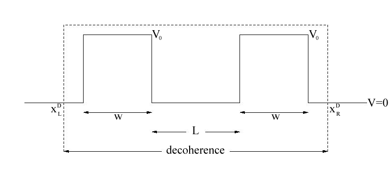
Figure 2: Double barrier case.

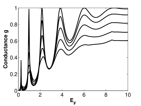
Figure 3: Conductance vs $E_{F}$ graph for different D values. D values are 0, 0.3, 0.5, 0.7, 0.9 from top right to bottom right.

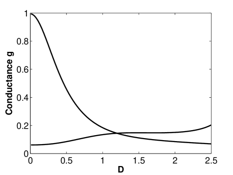
Figure 4: Conductance vs D graph for $E_{F}=E_{1}=0.96$ which is the second maximum at Conductance vs $E_{F}$ graph for different D values(Fig. 3) and for $E_{F}=E_{2}=1.41$ which is the second minimum in the same Fig. 3.

Fig. 3 shows conductance versus $E_{F}$ graph for different D values for the double barrier case. As seen in the figure the conductance decreases with the increase in decoherence. D=0 case is shown at the top. The peaks seen in the tunnelling region, where the energies are smaller than $V_{0}=2.5$, are due to resonant transmission. In this region we see that decoherence makes the constructive interference of electron waves disappears. After that region we see that conductance,i.e. the electron transmission, is suppressed by dephasing.

Fig. 4 shows conductance versus D graph for $E_{F}=E_{1}=0.96$ and for $E_{F}=E_{2}=1.41$ which is the second maximum and second minimum at Conductance vs $E_{F}$ graph for different D values(Fig. 3).

Decoherence mainly prevents wave interference. Depending on whether the interference increase or decrease the transmission probability, decoherence may decrease or increase the conductance. So, if constructive interference is present in the forward direction decoherence will prevent that and decrease the conductance. Otherwise, if destructive interference is effective in the forward direction, then decoherence increases the conductance. But as a rough guide we can give the following rule: When the transmission probability is roughly below 0.1, decoherence increases the conductance. Otherwise, if the transmission probability is above 0.1, then decoherence decreases the conductance.

In summary, we have proposed a model to address the significant dephasing effects in 1D transport.And we observe that dephasing can dramatically suppress the conductance of a conductor since it effects the transmission probability of the electron waves.

References

(1) S. Datta, Electronic Transport in Mesoscopic
Systems, Cambridge University Press, 1995
(2) C. Benjamin, A. M. Jayannavar,
cond-mat/0209438
(3) M. G. Pala and G. Iannaccone, Phys. Rev. B
69, 235304 (2004).
(4) M. Büttiker, Phys. Rev. B 33, 3020
(1986).
(5) M. Büttiker, IBM J. Res. Dev. 32, 63
(1988).
(6) X. Li and Y. Yan, Phys. Rev. B
65, 155326 (2002).
(7) C. W. J. Beenakker and B. Michaelis, J.
Phys. A: Math. Gen. 38, 10639 (2005).
(8) M. J. McLennan, Y. Lee and S. Datta, Phys. Rev. B
43, 13846 (1991).
(9) S. Hershfield, Phys. Rev. B 43, 11586 (1991).
(10) S. Datta, Phys. Rev. B 46, 9493 (1992).
(11) S. Datta, J. Phys. Condens. Matter 2, 8023 (1990).
(12) J. L. D’Amato and H. M. Pastawski. Phys. Rev. B 41, 7411 (1990).
(13) H. M. Pastawski. Phys. Rev. B 44, 6329 (1991).