TOPICS IN QUANTUM INFORMATION AND THE THEORY OF OPEN QUANTUM SYSTEMS

Dedication

To Iskra

Abstract

This thesis examines seven topics in quantum information and the theory of open quantum systems. The first topic concerns weak measurements and their universality as a means of generating quantum measurements. It is shown that every generalized measurement can be decomposed into a sequence of weak measurements which allows us to think of measurements as resulting form continuous stochastic processes. The second topic is an application of the decomposition into weak measurements to the theory of entanglement. Necessary and sufficient differential conditions for entanglement monotones are derived and are used to find a new entanglement monotone for three-qubit states. The third topic examines the performance of different master equations for the description of non-Markovian dynamics. The system studied is a qubit coupled to a spin bath via the Ising interaction. The fourth topic studies continuous quantum error correction in the case of non-Markovian decoherence. It is shown that due to the existence of a Zeno regime in non-Markovian dynamics, the performance of continuous quantum error correction may exhibit a quadratic improvement if the time resolution of the error-correcting operations is sufficiently high. The fifth topic concerns conditions for correctability of subsystem codes in the case of continuous decoherence. The obtained conditions on the Lindbladian and the system-environment Hamiltonian can be thought of as generalizations of the previously known conditions for noiseless subsystems to the case where the subsystem is time-dependent. The sixth topic examines the robustness of quantum error-correcting codes against initialization errors. It is shown that operator codes are robust against imperfect initialization without the need for restriction of the standard error-correction conditions. For this purpose, a new measure of fidelity for encoded information is introduced and its properties are discussed. The last topic concerns holonomic quantum computation and stabilizer codes. A fault-tolerant scheme for holonomic computations is presented, demonstrating the scalability of the holonomic method. The scheme opens the possibility for combining the benefits of error correction with the inherent resilience of the holonomic approach.

Chapter 1:   Introduction

1.1   Quantum information and open quantum systems

The field of quantum information and quantum computation has grown rapidly during the last two decades [115]. It has been shown that quantum systems can be used for information processing tasks that cannot be accomplished by classical means. Examples include quantum algorithms that can outperform the best known classical algorithms, such as Shor’s factoring algorithm [146] or Grover’s search algorithm [69], quantum communication protocols which use entanglement for teleportation of quantum states [19] or superdense coding [23], or quantum cryptographic protocols which offer provably secure ways of confidential key distribution between distant parties [18]. This has triggered an immense amount of research, leading to advances in many areas of quantum physics.

One area that has developed significantly as a result of the new growing field is that of open quantum systems. This development has been stimulated on one hand by the need to understand the full spectrum of operations that can be applied to a quantum state, as well as the information processing tasks that can be accomplished with them. Except for unitary transformations, which generally describe the dynamics of closed systems, the tools of quantum information science involve also measurements, completely positive (CP) maps [115], and even non-CP operations [141]. These more general operations result from interactions of the system of interest with auxiliary systems, and thus require knowledge of the dynamics of open quantum systems.

At the same time, it has been imperative to understand and find means to overcome the effects of noise on quantum information. Quantum superpositions, which are crucial for the workings of most quantum information processing schemes, can be easily destroyed by external interactions. This process, known as decoherence, has presented a major obstacle to the construction of reliable quantum information devices. This has prompted studies on the mechanisms of information loss in open quantum systems and the invention of methods to overcome them, giving rise to one of the pillars of quantum information science—the theory of quantum error correction [144, 150, 22, 89, 55, 176, 105, 103, 90, 51, 83, 174, 94, 95, 24].

Quantum error correction studies the information-preserving structures under open-system dynamics and the methods for encoding and processing of information using these structures. A major result in the theory of error correction states that if the error rate per information unit is below a certain value, by the use of fault-tolerant techniques and concatenation, an arbitrarily large information processing task can be implemented reliably with a modest overhead of resources [145, 53, 89, 2, 85, 91, 68, 67, 131]. This result, known as the accuracy threshold theorem, is of fundamental significance for quantum information science. It shows that despite the unavoidable effects of noise, scalable quantum information processing is possible in principle.

In this thesis, we examine topics from three intersecting areas in the theory open quantum systems and quantum information—the deterministic dynamics of open quantum systems, quantum measurements, and quantum error correction.

1.1.1   Deterministic dynamics of open quantum systems

All transformations in quantum mechanics, except for those that result from measurements, are usually thought of as arising from continuous evolution driven by a Hamiltonian that acts on the system of interest and possibly other systems. These transformations are therefore the result of the unitary evolution of a larger system that contains the system in question. Alternative interpretations are also possible—for example some transformation can be thought of as resulting from measurements whose outcomes are discarded. This description, however, can also be understood as originating from unitary evolution of a system which includes the measurement apparatus and all systems on which the outcome has been imprinted.

Including the environment in the description is generally difficult due to the large number of environment degrees of freedom. This is why it is useful to have a description which involves only the effective evolution of the reduced density operator of the system. When the system and the environment are initially uncorrelated, the effective evolution of the density operator of the system can be described by a completely positive trace-preserving (CPTP) linear map [93]. CPTP maps are widely used in quantum information science for describing noise processes and operations on quantum states [115]. They do not, however, describe the most general form of transformation of the state of an open system, since the initial state of the system and the environment can be correlated in a way which gives rise to non-CP transformations. Furthermore, the effective transformation by itself does not provide direct insights into the process that drives the transformation. For the latter one needs a description in terms of a generator of the evolution, similar to the way the Schrödinger equation describes the evolution of a closed system as generated by a Hamiltonian. The main difficulty in obtaining such a description for open systems is that the evolution of the reduced density matrix of the system is subject to non-trivial memory effects arising from the interaction with the environment [30].

In the limit where the memory of the environment is short-lived, the evolution of an open system can be described [30] by a time-local semi-group master equation in the Lindblad form [106]. Such an equation can be thought of as corresponding to a sequence of weak (infinitesimal) CPTP maps. When the memory of the environment cannot be ignored and the effective transformation on the initial state (which is not necessarily CP) is reversible, the evolution can be described by a time-local master equation, known as the time-convolutionless (TCL) master equation [143, 142]. In contrast to the Lindblad equation, this equation does not describe completely positive evolution.

The most general continuous deterministic evolution of an open quantum system is described by the Nakajima-Zwanzig (NZ) equation [112, 181]. This equation involves convolution in time. Both the TCL and NZ equations are quite complicated to obtain from first principles and are usually used for perturbative descriptions. Somewhere in between the Lindblad equation and the TCL or NZ equations are the phenomenological post-Markovian master equations such as the one proposed in Ref. [139].

In this thesis, we will examine the deterministic evolution of open quantum systems both from the point of view of the full evolution of the system and the environment and from the point of view of the reduced dynamics of the system. We will study the performance of different master equation for the description of the non-Markovian evolution of a qubit coupled to a spin bath [97], compare Markovian and non-Markovian models in light of continuous quantum error correction [120], and study the conditions for preservation of encoded information under Markovian evolution of the system and general Hamiltonian evolution of the system and the environment [122].

1.1.2   Quantum measurements

In addition to deterministic transformations, the state of an open quantum system can also undergo stochastic transformations. These are transformations for which the state may change in a number of different ways with non-unit probability. Since according to the postulates of quantum mechanics the only non-deterministic transformations are those that result from measurements [165, 108], stochastic transformations most generally result from measurements applied on the system and its environment. Just like deterministic transformations, stochastic transformations need not be completely positive. If the system of interest is initially entangled with its environment and after some joint unitary evolution of the system and the environment a measurement is performed on the environment, the effective transformation on the system resulting from this measurement need not be CP.

The class of completely positive stochastic operations are commonly referred to as generalized measurements [93]. Although this class includes standard projective measurements [165, 108] as well as other operations whose outcomes reveal information about the state, not all operations in this category reveal information. Some operations simply consist of deterministic operations applied with probabilities that do not depend on the state, i.e., they amount to trivial measurements.

In recent years, a special type of generalized quantum measurements, the so called weak measurements [4, 5, 99, 127, 6], have become of significant interest. A measurement is called weak if all of its outcomes result in small (infinitesimal) changes to the state. Weak measurements have been studied both in the abstract, and as a means of understanding systems with continuous monitoring. In the latter case, we can think of the evolution as the limit of a sequence of weak measurements, which gives rise to continuous stochastic evolutions called quantum trajectories (see, e.g., [41, 48, 61, 64, 52, 65, 129]). Such evolutions have been used also as models of decoherence (see, e.g., [32]). Weak measurements have found applications in feedback quantum control schemes [54] such as state preparation [74, 153, 154, 169, 46] or continuous quantum error correction [7, 135].

In this thesis, we look at weak measurements as a means of generating quantum transformations [118]. We show that any generalized measurement can be implemented as a sequence of weak measurements, which allows us to use the tools of differential calculus in studies concerning measurement-driven transformations. We apply this result to the theory of entanglement, deriving necessary and sufficient conditions for a function on quantum states to be an entanglement monotone [119]. We use these conditions to find a new entanglement monotone for three-qubit pure states, a subject of previously unsuccessful inquiries [63]. We also discuss the use of weak measurements for continuous quantum error correction.

1.1.3   Quantum error correction

Whether deterministic or stochastic, the evolution of a system coupled to its environment is generally irreversible. This is because the environment, by definition, is outside of the experimenter’s control. As irreversible transformations involve loss of information, they could be detrimental to a quantum information scheme unless an error-correcting method is employed.

A common form of error correction involves encoding the Hilbert space of a single information unit, say a qubit, in a subspace of the Hilbert space of a larger number of qubits [144, 150, 22, 89]. The encoding is such that if a single qubit in the code undergoes an error, the original state can be recovered by applying an appropriate operation. Clearly, there is a chance that more than one qubit undergoes an error, but according to the theory of fault tolerance [145, 53, 89, 2, 85, 91, 68, 67, 131] this problem can be dealt with by the use of fault-tolerant techniques and concatenation.

Error correction encompasses a wide variety of methods, each suitable for different types of noise, different tasks, or using different resources. Examples include passive error-correction methods which protect against correlated errors, such as decoherence-free subspaces [55, 176, 105, 103] and subsystems [90, 51, 83, 174], the standard active methods [144, 150, 22, 89] which are suitable for fault-tolerant computation [67], entanglement assisted quantum codes [34, 35] useful in quantum communication, or linear quantum error-correction codes [141] that correct non-completely positive errors. Recently, a general formalism called operator quantum error correction (OQEC) [94, 95, 24] was introduced, which unified in a common framework all previously proposed error-correction methods. This formalism employs the most general encoding of information—encoding in subsystems [88, 163]. OQEC was generalized to include entanglement-assisted error correction resulting in the most general quantum error-correction formalism presently known [73, 62].

In the standard formulation of error correction, noise and the error-correcting operations are usually represented by discrete transformations [94, 95, 24]. In practice, however, these transformations result from continuous processes. The more general situation where both the noise and the error-correcting processes are assumed to be continuous, is the subject of continuous quantum error correction [125, 136, 7, 135]. In the paradigm of continuous error correction, error-correcting operations are generated by weak measurements, weak unitary operations or weak completely positive maps. This approach often leads to a better performance in the setting of continuous decoherence than that involving discrete operations. In this thesis, we will discuss topics concerning both the discrete formalism and the continuous one. The topics we study include continuous quantum error correction for non-Markovian decoherence [120], conditions for correctability of operator codes under continuous decoherence [122], the performance of OQEC under imperfect encoding [117], as well as fault-tolerant computation based on holonomic operations [121].

1.2   Outline

This work examines seven topics in the areas of deterministic open-quantum-system dynamics, quantum measurements, and quantum error correction. Some of the topics concern all of these three themes, while others concern only two or only one. As each of the main results has a significance of its own, each topics has been presented as a separate study in one of the following chapters. The topics are ordered in view of the background material they introduce and the logical relation between them.

We first study the theme of weak measurements and their applications to the theory of entanglement. In Chapter 2, we show that every generalized quantum measurement can be generated as a sequence of weak measurements [118], which allows us to think of measurements in quantum mechanics as generated by continuous stochastic processes. In the case of two-outcome measurements, the measurement procedure has the structure of a random walk along a curve in state space, with the measurement ending when one of the end points is reached. In the continuous limit, this procedure corresponds to a quantum feedback control scheme for which the type of measurement is continuously adjusted depending on the measurement record. This result presents not only a practical prescription for the implementation of any generalized measurement, but also reveals a rich mathematical structure, somewhat similar to that of Lie algebras, which allows us to study the transformations caused by measurements by looking only at the properties of infinitesimal stochastic generators. The result suggests the possibility of constructing a unified theory of quantum measurement protocols.

Chapter 3 presents an application of the weak-measurement decomposition to a study of entanglement. The theory of entanglement concerns the transformations that are possible to a state under local operations and classical communication (LOCC). The universality of weak measurements allows us to look at LOCC as the class of transformations generated by infinitesimal local operations. We show that a necessary and sufficient condition for a function of the state to be an entanglement monotone under local operations that do not involve information loss is that the function be a monotone under infinitesimal local operations. We then derive necessary and sufficient differential conditions for a function of the state to be an entanglement monotone [119]. We first derive two conditions for local operations without information loss, and then show that they can be extended to more general operations by adding the requirement of convexity. We then demonstrate that a number of known entanglement monotones satisfy these differential criteria. We use the differential conditions to construct a new polynomial entanglement monotone for three-qubit pure states.

In Chapter 4, we extend the scope of our studies to include the deterministic dynamics of open quantum systems. We study the analytically solvable Ising model of a single qubit system coupled to a spin bath for a case for which the Markovian approximation of short bath-correlation times cannot be applied [97]. The purpose of this study is to analyze and elucidate the performance of Markovian and non-Markovian master equations describing the dynamics of the system qubit, in comparison to the exact solution. We find that the time-convolutionless master equation performs particularly well up to fourth order in the system-bath coupling constant, in comparison to the Nakajima-Zwanzig master equation. Markovian approaches fare poorly due to the infinite bath correlation time in this model. A recently proposed post-Markovian master equation performs comparably to the time-convolutionless master equation for a properly chosen memory kernel, and outperforms all the approximation methods considered here at long times. Our findings shed light on the applicability of master equations to the description of reduced system dynamics in the presence of spin baths.

In Chapter 5, we investigate further the difference between Markovian and non-Markovian decoherence—this time, form the point of view of its implications for the performance of continuous quantum error correction. We study the performance of a quantum-jump error correction model in the case where each qubit in a codeword is subject to a general Hamiltonian interaction with an independent bath [120]. We first consider the scheme in the case of a trivial single-qubit code, which provides useful insights into the workings of continuous error correction and the difference between Markovian and non-Markovian decoherence. We then study the model of a bit-flip code with each qubit coupled to an independent bath qubit and subject to continuous correction, and find its solution. We show that for sufficiently large error-correction rates, the encoded state approximately follows an evolution of the type of a single decohering qubit, but with an effectively decreased coupling constant. The factor by which the coupling constant is decreased scales quadratically with the error-correction rate. This is compared to the case of Markovian noise, where the decoherence rate is effectively decreased by a factor which scales only linearly with the rate of error correction. The quadratic enhancement depends on the existence of a Zeno regime in the Hamiltonian evolution which is absent in purely Markovian dynamics. We analyze the range of validity of this result and identify two relevant time scales. Finally, we extend the result to more general codes and argue that there the performance of continuous error correction will exhibit the same qualitative characteristics. In the appendix of this chapter, we discuss another application of weak measurements—we show how the quantum-jump error-correction scheme can be implemented using weak measurements and weak unitary operations.

In Chapter 6, we study the conditions under which a quantum code is perfectly correctable during a time interval of continuous decoherence for the most general type of encoding—encoding in subsystems. We study the case of Markovian decoherence as well as the general case of Hamiltonian evolution of the system and the environment, and derive necessary and sufficient conditions on the Lindbladian and the system-environment Hamiltonian [122], respectively. Our approach is based on a result obtained in Ref. [96] according to which a subsystem is correctable if and only if it is unitarily recoverable. The conditions we derive can be thought of as generalizations of the previously derived conditions for decoherence-free subsystems to the case where the subsystem is time-dependent. As a special case we consider conditions for unitary correctability. In the case of Hamiltonian evolution, the conditions for unitary correctability concern only the effect of the Hamiltonian on the system, whereas the conditions for general correctability concern the entire system-environment Hamiltonian. We also derive conditions on the Hamiltonian which depend on the initial state of the environment. We discuss possible implications of our results for approximate quantum error correction.

Chapter 7 also concerns subsystem codes. Here we study the performance of operator quantum error correction (OQEC) in the case of imperfect encoding [117]. In the OQEC, the notion of correctability is defined under the assumption that states are perfectly initialized inside a particular subspace, a factor of which (a subsystem) contains the protected information. It was believed that in the case of imperfect initialization, OQEC codes would require more restrictive than the standard conditions if they are to protect encoded information from subsequent errors. In this chapter, we examine this requirement by looking at the errors on the encoded state. In order to quantitatively analyze the errors in an OQEC code, we introduce a measure of the fidelity between the encoded information in two states for the case of subsystem encoding. A major part of the chapter concerns the definition of the measure and the derivation of its properties. In contrast to what was previously believed, we obtain that more restrictive conditions are not necessary neither for DFSs nor for general OQEC codes. This is because the effective noise that can arise inside the code as a result of imperfect initialization is such that it can only increase the fidelity of an imperfectly encoded state with a perfectly encoded one.

In Chapter 8, we present a scheme for fault-tolerant holonomic computation on stabilizer codes [121]. In the holonomic approach, logical states are encoded in the degenerate eigenspace of a Hamiltonian and gates are implemented by adiabatically varying the Hamiltonian along loops in parameter space. The result is a transformation of purely geometric origin, which is robust against various types of errors in the control parameters driving the evolution. In the proposed scheme, single-qubit operations on physical qubits are implemented by varying Hamiltonians that are elements of the stabilizer, or in the case of subsystem codes—elements of the gauge group. By construction, the geometric transformations in each eigenspace of the Hamiltonian are transversal, which ensures that errors do not propagate. We show that for certain codes, such as the nine-qubit Shor code or its subsystem versions, it is possible to realize universal fault-tolerant computation using Hamiltonians of weight three. The scheme proves that holonomic quantum computation is a scalable method and opens the possibility for bringing together the benefits of error correction and the operational robustness of the holonomic approach. It also presents an alternative to the standard fault-tolerant methods based on dynamical transformations, which have been argued to be in a possible conflict with the assumption of Markovian decoherence that often underlies the derivation of threshold results.

Chapter 9 summarizes the results and discusses problems for future research.

Chapter 2:   Generating quantum measurements using weak measurements

2.1   Preliminaries

In the original formulation of measurement in quantum mechanics, measurement outcomes are identified with a set of orthogonal projection operators, which can be thought of as corresponding to the eigenspaces of a Hermitian operator, or observable [165, 108]. After a measurement, the state is projected into one of the subspaces with a probability given by the square of the amplitude of the state’s component in that subspace.

In recent years a more general notion of measurement has become common: the so called generalized measurement which corresponds to a positive operator valued measure (POVM) [93]. This formulation can include many phenomena not captured by projective measurements: detectors with non-unit efficiency, measurement outcomes that include additional randomness, measurements that give incomplete information, and many others. Generalized measurements have found numerous applications in the rapidly-growing field of quantum information processing [115]. Some examples include protocols for unambiguous state discrimination [126] and optimal entanglement manipulation [114, 76].

Upon measurement, a system with density matrix $\rho$ undergoes a random transformation

$$\rho\rightarrow\rho_{j}={M}_{j}\rho{M}_{j}^{\dagger}/p_{j},\hskip 11.38092pt\underset{j}{\sum}{M}_{j}^{\dagger}{M}_{j}={I},$$ (1)

with probability $p_{j}=\textrm{Tr}({M}_{j}\rho{M}_{j}^{\dagger})$, where the index $j$ labels the possible outcomes of the measurement. Eq. (1) is not the most general stochastic operation that can be applied to a state. For example, one can consider the transformation

$$\rho\rightarrow\rho_{j}=\underset{i}{\sum}{M}_{ij}\rho{M}_{ij}^{\dagger}/p_{j},\hskip 11.38092pt\underset{i,j}{\sum}{M}_{ij}^{\dagger}{M}_{ij}={I},$$ (2)

where $p_{j}=\textrm{Tr}(\underset{i}{\sum}{M}_{ij}\rho{M}_{ij}^{\dagger})$ is the probability for the $j^{\textrm{th}}$ outcome (see Chapter 3). The letter can be thought of as resulting from a measurement of the type (1) with measurement operators $M_{ij}$ of which only the information about the index $j$ labeling the outcome is retained. In this thesis, when we talk about generalized measurements, we will refer to the transformation (1).

The transformation (1) is commonly comprehended as a spontaneous jump, unlike unitary transformations, for example, which are thought of as resulting from continuous unitary evolutions. Any unitary transformation can be implemented as a sequence of weak (i.e., infinitesimal) unitary transformations. One may ask if a similar decomposition exists for generalized measurements. This would allow us to think of generalized measurements as resulting from continuous stochastic evolutions and possibly make use of the powerful tools of differential calculus in the study of the transformations that a system undergoes upon measurement.

In this chapter we show that any generalized measurement can be implemented as a sequence of weak measurements and present an explicit form of the decomposition. The main result was first presented in Ref. [118]. We call a measurement weak if all outcomes result in very small changes to the state. (There are other definitions of weak measurements that include the possibility of large changes to the state with low probability; we will not be considering measurements of this type.) Therefore, a weak measurement is one whose operators can be written as

$${M}_{j}=q_{j}({I}+{\varepsilon}_{j}),$$ (3)

where $q_{j}\in{C}$, $0\leq|q_{j}|\leq 1$, and ${\varepsilon}$ is an operator with small norm $\|{\varepsilon}\|\ll 1$.

2.2   Decomposing projective measurements

It has been shown that any projective measurement can be implemented as a sequence of weak measurements; and by using an additional ancilla system and a joint unitary transformation, it is possible to implement any generalized measurement using weak measurements [21]. This procedure, however, does not decompose the operation on the original system into weak operations, since it uses operations acting on a larger Hilbert space—that of the system plus the ancilla. If we wish to study the behavior of a function—for instance, an entanglement monotone—defined on a space of a particular dimension, it complicates matters to add and remove ancillas. We will show that an ancilla is not needed, and give an explicit construction of the weak measurement operators for any generalized measurement that we wish to decompose.

It is easy to show that a measurement with any number of outcomes can be performed as a sequence of measurements with two outcomes. Therefore, for simplicity, we will restrict our considerations to two-outcome measurements. To give the idea of the construction, we first show how every projective measurement can be implemented as a sequence of weak generalized measurements. In this case the measurement operators ${P}_{1}$ and ${P}_{2}$ are orthogonal projectors whose sum ${P}_{1}+{P}_{2}={I}$ is the identity. We introduce the operators

$${P}(x)=\sqrt{\frac{1-\tanh(x)}{2}}{P}_{1}+\sqrt{\frac{1+\tanh(x)}{2}}{P}_{2},\hskip 14.22636ptx\in R.$$ (4)

Note that ${P}^{2}(x)+{P}^{2}(-x)={I}$ and therefore ${P}(x)$ and ${P}(-x)$ describe a measurement. If $x=\epsilon$, where $|\epsilon|\ll 1$, the measurement is weak. Consider the effect of the operators ${P}(x)$ on a pure state $|\psi\rangle$. The state can be written as $|\psi\rangle={P}_{1}|\psi\rangle+{P}_{2}|\psi\rangle=\sqrt{p_{1}}|\psi_{1}\rangle+\sqrt{p_{2}}|\psi_{2}\rangle$, where $|\psi_{1,2}\rangle={P}_{1,2}|\psi\rangle/\sqrt{p_{1,2}}$ are the two possible outcomes of the projective measurement and $p_{1,2}=\langle\psi|{P}_{1,2}|\psi\rangle$ are the corresponding probabilities. If $x$ is positive (negative), the operator ${P}(x)$ increases (decreases) the ratio $\sqrt{p_{2}}/\sqrt{p_{1}}$ of the $|\psi_{2}\rangle$ and $|\psi_{1}\rangle$ components of the state. By applying the same operator ${P}(\epsilon)$ many times in a row for some fixed $\epsilon$, the ratio can be made arbitrarily large or small depending on the sign of $\epsilon$, and hence the state can be transformed arbitrarily close to $|\psi_{1}\rangle$ or $|\psi_{2}\rangle$. The ratio of the $p_{1}$ and $p_{2}$ is the only parameter needed to describe the state, since $p_{1}+p_{2}=1$.

Also note that ${P}(-x){P}(x)=(1-\tanh^{2}(x))^{1/2}{I}/2$ is proportional to the identity. If we apply the same measurement ${P}(\pm\epsilon)$ twice and two opposite outcomes occur, the system returns to its previous state. Thus we see that the transformation of the state under many repetitions of the measurement ${P}(\pm\epsilon)$ follows a random walk along a curve ${|\psi(x)\rangle}$ in state space. The position on this curve can be parameterized by $x=\ln\sqrt{p_{1}/p_{2}}$. Then ${|\psi(x)\rangle}$ can be written as $\sqrt{p_{1}(x)}{|\psi_{1}\rangle}+\sqrt{p_{2}(x)}{|\psi_{2}\rangle}$, where $p_{1,2}(x)=(1/2)[1\pm\tanh(x)]$.

The measurement given by the operators ${P}(\pm\epsilon)$ changes $x$ by $x\rightarrow x\pm\epsilon$, with probabilities $p_{\pm}(x)=(1\pm\tanh(\epsilon)(p_{1}(x)-p_{2}(x)))/2$. We continue this random walk until $|x|\geq X$, for some $X$ which is sufficiently large that ${|\psi(X)\rangle}\approx{|\psi_{1}\rangle}$ and ${|\psi(-X)\rangle}\approx{|\psi_{2}\rangle}$ to whatever precision we desire. What are the respective probabilities of these two outcomes?

Define $p(x)$ to be the probability that the walk will end at $X$ (rather than $-X$) given that it began at $x$. This must satisfy $p(x)=p_{+}(x)p(x+\epsilon)+p_{-}(x)p(x-\epsilon)$. Substituting our expressions for the probabilities, this becomes

$$p(x)=(p(x+\epsilon)+p(x-\epsilon))/2+\tanh(\epsilon)\tanh(x)(p(x+\epsilon)-p(x-\epsilon))/2.$$ (5)

If we go to the infinitesimal limit $\epsilon\rightarrow dx$, this becomes a continuous differential equation

$$\frac{d^{2}p}{dx^{2}}+2\tanh(x)\frac{dp}{dx}=0,$$ (6)

with boundary conditions $p(X)=1$, $p(-X)=0$. The solution to this equation is $p(x)=(1/2)[1+\tanh(x)/\tanh(X)]$. In the limit where $X$ is large, $\tanh(X)\rightarrow 1$, so $p(x)=p_{1}(x)$. The probabilities of the outcomes for the sequence of weak measurements are exactly the same as those for a single projective measurement. Note that this is also true for a walk with a step size that is not infinitesimal, since the solution $p(x)$ satisfies (5) for an arbitrarily large $\epsilon$.

Alternatively, instead of looking at the state of the system during the process, we could look at an operator that effectively describes the system’s transformation to the current state. This has the advantage that it is state-independent, and will lead the way to decompositions of generalized measurements; it also becomes obvious that the procedure works for mixed states, too.

We think of the measurement process as a random walk along a curve ${P}(x)$ in operator space, given by Eq. (4), which satisfies ${P}(0)={I}/\sqrt{2}$, $\underset{x\rightarrow-\infty}{\lim}{P}(x)={P}_{1}$, $\underset{x\rightarrow\infty}{\lim}{P}(x)={P}_{2}$. It can be verified that ${P}(x){P}(y)\propto{P}(x+y)$, where the constant of proportionality is $(\cosh(x+y)/2\cosh(x)\cosh(y))^{1/2}$. Due to normalization of the state, operators which differ by an overall factor are equivalent in their effects on the state. Thus, the random walk driven by weak measurement operators ${P}(\pm\epsilon)$ has a step size $|\epsilon|$.

2.3   Decomposing generalized measurements

Next we consider measurements where the measurement operators ${M}_{1}$ and ${M}_{2}$ are positive but not projectors. We use the well known fact that a generalized measurement can be implemented as joint unitary operation on the system and an ancilla, followed by a projective measurement on the ancilla [115]. (One can think of this as an indirect measurement; one lets the system interact with the ancilla, and then measures the ancilla.) Later we will show that the ancilla is not needed. We consider two-outcome measurements and two-level ancillas. In this case ${M}_{1}$ and ${M}_{2}$ commute, and hence can be simultaneously diagonalized.

Let the system and ancilla initially be in a state $\rho\otimes|0\rangle\langle 0|$. Consider the unitary operation

$${U}(0)={M}_{1}\otimes{Z}+{M}_{2}\otimes{X},$$ (7)

where ${X}=\sigma^{x}$ and ${Z}=\sigma^{z}$ are Pauli matrices acting on the ancilla bit. By applying ${U}(0)$ to the extended system we transform it to:

$${U}(0)(\rho\otimes|0\rangle\langle 0|){U}^{\dagger}(0) = {M}_{1}\rho{M}_{1}\otimes|0\rangle\langle 0|+{M}_{1}\rho{M}_{2}\otimes|0\rangle\langle 1|$$ (8)

$$+ {M}_{2}\rho{M}_{1}\otimes|1\rangle\langle 0|+{M}_{2}\rho{M}_{2}\otimes|1\rangle\langle 1|.$$

Then a projective measurement on the ancilla in the computational basis would yield one of the possible generalized measurement outcomes for the system. We can perform the projective measurement on the ancilla as a sequence of weak measurements by the procedure we described earlier. We will then prove that for this process, there exists a corresponding sequence of generalized measurements with the same effect acting solely on the system. To prove this, we first show that at any stage of the measurement process, the state of the extended system can be transformed into the form $\rho(x)\otimes|0\rangle\langle 0|$ by a unitary operation which does not depend on the state.

The net effect of the joint unitary operation ${U}(0)$, followed by the effective measurement operator on the ancilla, can be written in a block form in the computational basis of the ancilla:

$${\bar{M}}(x) \equiv ({I}\otimes{P}(x)){U}(0)=\begin{pmatrix}\sqrt{\frac{1-\tanh(x)}{2}}{M}_{1}&\sqrt{\frac{1-\tanh(x)}{2}}{M}_{2}\\ \sqrt{\frac{1+\tanh(x)}{2}}{M}_{2}&-\sqrt{\frac{1+\tanh(x)}{2}}{M}_{1}\end{pmatrix}.$$ (9)

If the current state ${\bar{M}}(x)(\rho\otimes|0\rangle\langle 0|){\bar{M}}^{\dagger}$ can be transformed to $\rho(x)\otimes|0\rangle\langle 0|$ by a unitary operator ${U}(x)$ which is independent of $\rho$, then the lower left block of ${U}(x){\bar{M}}(x)$ should vanish. We look for such a unitary operator in block form, with each block being Hermitian and diagonal in the same basis as ${M_{1}}$ and ${M_{2}}$. One solution is:

$${U}(x)=\begin{pmatrix}{A}(x)&{B}(x)\\ {B}(x)&-{A}(x)\end{pmatrix},$$ (10)

where

$${A}(x)=\sqrt{1-\tanh(x)}{M}_{1}({I}+\tanh(x)({M}_{2}^{2}-{M}_{1}^{2}))^{-\frac{1}{2}},$$ (11)

$${B}(x)=\sqrt{1+\tanh(x)}{M}_{2}({I}+\tanh(x)({M}_{2}^{2}-{M}_{1}^{2}))^{-\frac{1}{2}}.$$ (12)

(Since ${M}_{1}^{2}+{M}_{2}^{2}={I}$, the operator $({I}+\tanh(x)({M}_{2}^{2}-{M}_{1}^{2}))^{-\frac{1}{2}}$ always exists.) Note that ${U}(x)$ is Hermitian, so ${U}(x)={U}^{\dagger}(x)$ is its own inverse, and at $x=0$ it reduces to the operator (7).

After every measurement on the ancilla, depending on the value of $x$, we apply the operation ${U}(x)$. Then, before the next measurement, we apply its inverse ${U}^{\dagger}(x)={U}(x)$. By doing this, we can think of the procedure as a sequence of generalized measurements on the extended system that transform it between states of the form $\rho(x)\otimes|0\rangle\langle 0|$ (a generalized measurement preceded by a unitary operation and followed by a unitary operation dependent on the outcome is again a generalized measurement). The measurement operators are now ${\tilde{M}}(x,\pm\epsilon)\equiv{U}(x\pm\epsilon)({I}\otimes{P}(\pm\epsilon)){U}(x)$, and have the form

$${\tilde{M}}(x,\pm\epsilon)=\begin{pmatrix}{M}(x,\pm\epsilon)&{N}(x,\pm\epsilon)\\ {0}&{O}(x,\pm\epsilon)\end{pmatrix}.$$ (13)

Here ${M},{N},{O}$ are operators acting on the system. Upon measurement, the state of the extended system is transformed

$$\rho(x)\otimes|0\rangle\langle 0|\rightarrow\frac{{M}(x,\pm\epsilon)\rho(x){M}^{\dagger}(x,\pm\epsilon)}{p(x,\pm\epsilon)}\otimes|0\rangle\langle 0|,$$ (14)

with probability

$$p(x,\pm\epsilon)={\rm Tr}\left\{{M}(x,\pm\epsilon)\rho(x){M}^{\dagger}(x,\pm\epsilon)\right\}.$$ (15)

By imposing ${\tilde{M}}^{\dagger}(x,\epsilon){\tilde{M}}(x,\epsilon)+{\tilde{M}}(x,-\epsilon)^{\dagger}{\tilde{M}}(x,-\epsilon)={I}$, we obtain that

$${M}^{\dagger}(x,\epsilon){M}(x,\epsilon)+{M}^{\dagger}(x,-\epsilon){M}(x,-\epsilon)={I},$$ (16)

where the operators in the last equation acts on the system space alone. Therefore, the same transformations that the system undergoes during this procedure can be achieved by the measurements ${M}(x,\pm\epsilon)$ acting solely on the system. Depending on the current value of $x$, we perform the measurement ${M}(x,\pm\epsilon)$. Due to the one-to-one correspondence with the random walk for the projective measurement on the ancilla, this procedure also follows a random walk with a step size $|\epsilon|$. It is easy to see that if the measurements on the ancilla are weak, the corresponding measurements on the system are also weak. Therefore we have shown that every measurement with positive operators ${M}_{1}$ and ${M}_{2}$, can be implemented as a sequence of weak measurements. This is the main result of this chapter. From the construction above, one can find the explicit form of the weak measurement operators:

$${M}(x,\epsilon)=\sqrt{\frac{1-\tanh(\epsilon)}{2}}{A}(x){A}(x+\epsilon)+\sqrt{\frac{1+\tanh(\epsilon)}{2}}{B}(x){B}(x+\epsilon).$$ (17)

These expressions can be simplified further. The current state of the system at any point during the procedure can be written as

$${M}(x)\rho{M}(x)/{\rm Tr}({M}^{2}(x)\rho),$$ (18)

where

$${M}(x)=\sqrt{\frac{{I}+\tanh(x)({M}_{2}^{2}-{M}_{1}^{2})}{2}},\ \ x\in R.$$ (19)

The weak measurement operators can be written as

$${M}(x,\pm\epsilon)=\sqrt{C_{\pm}\frac{{I}+\tanh(x\pm\epsilon)({M}_{2}^{2}-{M}_{1}^{2})}{{I}+\tanh(x)({M}_{2}^{2}-{M}_{1}^{2})}},$$ (20)

where the weights $C_{\pm}$ are chosen to ensure that these operators form a generalized measurement:

$$C_{\pm}=(1\pm\tanh(\epsilon)\tanh(x))/2.$$ (21)

Note that this procedure works even if the step of the random walk is not small, since ${P}(x){P}(y)\propto{P}(x+y)$ for arbitrary values of $x$ and $y$. So it is not surprising that the effective operator which gives the state of the system at the point $x$ is ${M}(x)\equiv{M}(0,x)$.

In the limit when $\epsilon\rightarrow 0$, the evolution under the described procedure can be described by a continuous stochastic equation. We can introduce a time step $\delta t$ and a rate

$$\gamma=\epsilon^{2}/\delta t.$$ (22)

Then we can define a mean-zero Wiener process $\delta W$ as follows:

$$\delta W=(\delta x-M[\delta x])/\sqrt{\gamma},$$ (23)

where $M[\delta x]$ is the mean of $\delta x$,

$$M[\delta x]=\epsilon(p_{+}(x)-p_{-}(x)).$$ (24)

The probabilities $p_{\pm}(x)$ can be written in the form

$$p_{\pm}(x)=\frac{1}{2}(1\pm 2\langle{Q}(x)\rangle\epsilon),$$ (25)

where $\langle{Q}(x)\rangle$ denotes the expectation value of the operator

$$Q(x)=\frac{1}{2}\frac{({M}_{2}^{2}-{M}_{1}^{2})+\tanh(x){I}}{{I}+\tanh(x)({M}_{2}^{2}-{M}_{1}^{2})}.$$ (26)

Note that $M[(\delta W)^{2}]=\delta t+\textit{O}(\delta t^{2})$. Expanding the change of a state $|\psi\rangle$ upon the measurement ${M}(x,\pm\epsilon)$ up to second order in $\delta W$ and taking the limit $\delta W\rightarrow 0$ averaging over many steps, we obtain the following coupled stochastic differential equations:

$$|d\psi\rangle=-\frac{\gamma}{2}({Q}(x)-\langle{Q}(x)\rangle)^{2}|\psi\rangle dt+\sqrt{\gamma}({Q}(x)-\langle{Q}(x)\rangle)|\psi\rangle dW,$$ (27)

$$dx=2\gamma\langle{Q}(x)\rangle dt+\sqrt{\gamma}dW.$$ (28)

This process corresponds to a continuous measurement of an observable ${Q}$ which is continuously changed depending on the value of $x$. In other words, it is a feedback-control scheme where depending on the measurement record, the type of measurement is continuously adjusted.

Finally, consider the most general type of two-outcome generalized measurement, with the only restriction being ${M}_{1}^{\dagger}{M}_{1}+{M}_{2}^{\dagger}{M}_{2}=I$. By polar decomposition the measurement operators can be written

$${M}_{1,2}={V}_{1,2}\sqrt{{M}_{1,2}^{\dagger}{M}_{1,2}},$$ (29)

where ${V}_{1,2}$ are appropriate unitary operators. One can think of these unitaries as causing an additional disturbance to the state of the system, in addition to the reduction due to the measurement. The operators $({M}_{1,2}^{\dagger}{M}_{1,2})^{1/2}$ are positive, and they form a measurement. We could then measure ${M}_{1}$ and ${M}_{2}$ by first measuring these positive operators by a sequence of weak measurements, and then performing either ${V}_{1}$ or ${V}_{2}$, depending on the outcome.

However, we can also decompose this measurement directly into a sequence of weak measurements. Let the weak measurement operators for $({M}_{1,2}^{\dagger}{M}_{1,2})^{1/2}$ be ${M}_{p}(x,\pm\epsilon)$. Let ${V}(x)$ be any continuous unitary operator function satisfying ${V}(0)={I}$ and ${V}(\pm x)\rightarrow{V}_{1,2}$ as $x\rightarrow\infty$. We then define

$${M}(x,y)\equiv{V}(x+y){M}_{p}(x,y){V}^{\dagger}(x).$$ (30)

By construction ${M}(x,\pm y)$ are measurement operators. Since ${V}(x)$ is continuous, if $y=\epsilon$, where $\epsilon\ll 1$, the measurements are weak. The measurement procedure is analogous to the previous cases and follows a random walk along the curve ${M}(0,x)={V}(x){M}_{p}(0,x)$.

In summary, we have shown that for every two-outcome measurement described by operators ${M}_{1}$ and ${M}_{2}$ acting on a Hilbert space of dimension $d$, there exists a continuous two-parameter family of operators ${M}(x,y)$ over the same Hilbert space with the following properties:

$${M}(x,0)={I}/\sqrt{2},$$ (31)

$${M}(0,x)\rightarrow{M}_{1}\hskip 5.69046pt\textrm{as}\hskip 5.69046ptx\rightarrow-\infty,$$ (32)

$${M}(0,x)\rightarrow{M}_{2}\hskip 5.69046pt\textrm{as}\hskip 5.69046ptx\rightarrow+\infty,$$ (33)

$${M}(x+y,z){M}(x,y)\propto{M}(x,z+y),$$ (34)

$${M}^{\dagger}(x,y){M}(x,y)+{M}^{\dagger}(x,-y){M}(x,-y)={I}.$$ (35)

We have presented an explicit solution for ${M}(x,y)$ in terms of ${M}_{1}$ and ${M}_{2}$. The measurement is implemented as a random walk on the curve ${M}(0,x)$ by consecutive application of the measurements ${M}(x,\pm\epsilon)$, which depend on the current value of the parameter $x$. In the case where $|\epsilon|\ll 1$, the measurements driving the random walk are weak. Since any measurement can be decomposed into two-outcome measurements, weak measurements are universal.

2.4   Measurements with multiple outcomes

Even though two-outcome measurements can be used to construct any multi-outcome measurement, it is interesting whether a direct decomposition similar to the one we presented can be obtained for measurements with multiple outcomes as well. In Ref. [159] it was shown that such a decomposition exists. For a measurement with $n$ positive operators ${L}_{j}$, $j=1,...,n$, $\overset{n}{\underset{j=1}{\sum}}{L}_{j}^{2}=I$, the effective measurement operator $M(x)$ describing the state during the procedure is given by [159]

$$M(s)=\sqrt{f(s)}\sqrt{(\overset{n}{\underset{j=1}{\sum}}s^{j}L_{j}^{2})},$$ (36)

where

$$f(s)=1+n\overset{n}{\underset{j=1}{\sum}}s^{j}(1-s^{j}).$$ (37)

Here the parameter $s$ is chosen such that $\overset{n}{\underset{j=1}{\sum}}s^{j}=1$, $s\in[0,1]$, i.e., it describes a simplex. The system of stochastic equations describing the process in the case when the measurement operators ${L}_{j}$ are commuting, can be written as

$$|d\psi\rangle=-\frac{\gamma}{8}g^{jk}(s)({Q}_{j}(s)-\langle{Q}_{j}(s)\rangle)({Q}_{k}(s)-\langle{Q}_{k}(s)\rangle)|\psi\rangle dt+$$

$$\frac{1}{2}\sqrt{\gamma}({Q_{i}}(s)-\langle{Q_{i}}(s)\rangle)|\psi\rangle a^{i}_{\alpha}(s)dW^{\alpha},$$ (38)

$$ds=\gamma g^{ij}(s)\langle{Q}_{j}(s)\rangle dt+\sqrt{\gamma}a^{i}_{\alpha}(s)dW^{\alpha},$$ (39)

where

$${Q_{i}}(s)=\frac{L_{i}^{2}}{s^{m}L_{m}^{2}},$$ (40)

$$g^{ij}(s)=\overset{n}{\underset{\alpha,\beta=1}{\sum}}s^{i}(\delta^{i}_{\alpha}-s^{\alpha})(\delta^{\alpha}_{\beta}-\frac{1}{n})s^{j}(\delta^{j}_{\beta}-s^{\beta}),$$ (41)

$a(s)$ is the square root of $g(s)$,

$$g^{ij}(s)=\overset{n}{\underset{k=1}{\sum}}a_{k}^{i}(s)a_{k}^{j}(s),$$ (42)

and we have assumed Einstein’s summation convention.

The decomposition can be easily generalized to the case of non-positive measurement operators in a way similar to the one we described for the two-outcome case—by inserting suitable weak unitaries between the weak measurements.

2.5   Summary and outlook

The result presented in this chapter may have important implications for quantum control and the theory of quantum measurements in general. It provides a practical prescription for the implementation of any generalized measurement using weak measurements which may be useful in experiments where strong measurements are difficult to implement. The decomposition might be experimentally feasible for some quantum optical or atomic systems.

The result also reveals an interesting mathematical structure, somewhat similar to that of Lie algebras, which allows us to think of measurements as generated by infinitesimal stochastic generators. One application of this is presented in the following chapter, where we derive necessary and sufficient conditions for a function on quantum states to be an entanglement monotone. An entanglement monotone [161] is a function which does not increasing on average under local operations. For pure states the operations are unitaries and generalized measurements. Since all unitaries can be broken into a series of infinitesimal steps and all measurements can be decomposed into weak measurements, it suffices to look at the behavior of a prospective monotone under small changes in the state. Thus we can use this result to derive differential conditions on the function.

These observations suggest that it may be possible to find a unified description of quantum operations where every quantum operations can be continuously generated. Clearly, measurements do not form a group since they do not have inverse elements, but it may be possible to describe them in terms of a semi-group. The problem with using measurements as the elements of the semigroup is that a strong measurement is not equal to a composition of weak measurements, since the sequence of weak measurements that builds up a particular strong measurement is not pre-determined—the measurements depend on a stochastic parameter. It may be possible, however, to use more general objects—measurement protocols—which describe measurements applied conditioned on a parameter in some underlying manifold. If such a manifold exists for the most general possible notion of a protocol, the basic objects could be describable by stochastic matrices on this manifold. Such a possibility is appealing since stochastic processes are well understood and this may have important implications for the study of quantum control protocols. In addition, such a description could be useful for describing general open-system dynamics. These questions are left open for future investigation.

Chapter 3:   Applications of the decomposition into weak measurements to the theory of entanglement

3.1   Preliminaries

In this chapter we apply the result on the universality of weak measurements to the theory of entanglement. The theory of entanglement concerns the transformations that are possible to a state under local operations with classical communication (LOCC). The paradigmatic experiment is a quantum system comprising several subsystems, each in a separate laboratory under control of a different experimenter: Alice, Bob, Charlie, etc. Each experimenter can perform any physically allowed operation on his or her subsystem—unitary transformations, generalized measurements, indeed any trace-preserving completely positive operation–and communicate their results to each other without restriction. They are not, however, allowed to bring their subsystems together and manipulate them jointly. An LOCC protocol consists of any number of local operations, interspersed with any amount of classical communication; the choice of operations at later times may depend on the outcomes of measurements at any earlier time.

The results of Bennett et al. [17, 20, 22] and Nielsen [114], among many others [160, 76, 72, 77, 162], have given us a nearly complete theory of entanglement for bipartite systems in pure states. Unfortunately, great difficulties have been encountered in trying to extend these results both to mixed states and to states with more than two subsystems (multipartite systems). The reasons for this are many; but one reason is that the set LOCC is complicated and difficult to describe mathematically [21].

One mathematical tool which has proven very useful is that of the entanglement monotone: a function of the state which is invariant under local unitary transformations and always decreases (or increases) on average after any local operation. These functions were described by Vidal [161], and large classes of them have been enumerated since then.

We will consider those protocols in LOCC that preserve pure states as the set of operations generated by infinitesimal local operations: operations which can be performed locally and which leave the state little changed including infinitesimal local unitaries and weak generalized measurements. In Bennett et al. [21] it was shown that infinitesimal local operations can be used to perform any local operation with the additional use of local ancillary systems–extra systems residing in the local laboratories, which can be coupled to the subsystems for a time and later discarded. As we saw in the previous section, any local generalized measurement can be implemented as a sequence of weak measurements without the use of ancillas. This implies that a necessary and sufficient condition for a function of the state to be a monotone under local operations that preserve pure states is the function to be a monotone under infinitesimal local operations.

In this chapter we derive differential conditions for a function of the state to be an entanglement monotone by considering the change of the function on average under infinitesimal local operations up to the lowest order in the infinitesimal parameter. We thus obtain conditions that involve at most second derivatives of the function. We then prove that these conditions are both necessary and sufficient. We show that the conditions are satisfied by a number of known entanglement monotones and we use them to construct a new polynomial entanglement monotone for three-qubit pure states.

We hope that this approach will provide a new window with which to study LOCC, and perhaps avoid some of the difficulties in the theory of multipartite and mixed-state entanglement. By looking only at the differential behavior of entanglement monotones, we avoid concerns about the global structure of LOCC or the class of separable operations.

In Section 3.2, we define the basic concepts of this chapter: LOCC operations, entanglement monotones, and infinitesimal operations. In Section 3.3, we show how all local operations that preserve pure states can be generated by a sequence of infinitesimal local operations. In Section 3.4, we derive differential conditions for a function of the state to be an entanglement monotone. There are two such conditions for pure-state entanglement monotones: the first guarantees invariance under local unitary transformations (LU invariance), and involves only the first derivatives of the function, while the second guarantees monotonicity under local measurements, and involves second derivatives. For mixed-state entanglement monotones we add a further condition, convexity, which ensures that a function remains monotonic under operations that lose information (and can therefore transform pure states to mixed states). In Section 3.5, we look at some known monotones–the norm of the state, the local purity, and the entropy of entanglement–and show that they obey the differential criteria. In Section 3.6, we use the differential conditions to construct a new polynomial entanglement monotone for three-qubit pure states which depends on the invariant identified by Kempe [82]. In Section 3.7 we conclude. In the Appendix (Section 3.8), we show that higher derivatives of the function are not needed to prove monotonicity.

3.2   Basic definitions

3.2.1   LOCC

An operation (or protocol) in LOCC consists of a sequence of local operations with classical communication between them. Initially, we will consider only those local operations that preserve pure states: unitaries, in which the state is transformed

$$\rho\rightarrow{U}\rho{U}^{\dagger},\ \ {U}^{\dagger}{U}={U}{U}^{\dagger}={I},$$ (43)

and generalized measurements, in which the state randomly changes as in Eq. (1),

$$\rho\rightarrow\rho_{j}={M}_{j}\rho{M}^{\dagger}_{j}/p_{j},\ \ \sum_{j}{M}^{\dagger}_{j}{M}_{j}={I},$$

with probability $p_{j}={\rm Tr}\left\{{M}^{\dagger}_{j}{M}_{j}\rho\right\}$, where the index $j$ labels the possible outcomes of the measurement. Note that we can think of a unitary as being a special case of a generalized measurement with only one possible outcome. One can think of this class of operations as being limited to those which do not discard information. Later, we will relax this assumption to consider general operations, which can take pure states to mixed states. Such operations do involve loss of information. Examples include performing a measurement without retaining the result, performing an unknown unitary chosen at random, or entangling the system with an ancilla which is subsequently discarded.

The requirement that an operation be local means that the operators ${U}$ or ${M}_{j}$ must have a tensor-product structure ${U}\equiv{U}\otimes{I}$, ${M}_{j}\equiv{M}_{j}\otimes{I}$, where they act as the identity on all except one of the subsystems. The ability to use classical communication implies that the choice of later local operations can depend arbitrarily on the outcomes of all earlier measurements. One can think of an LOCC operation as consisting of a series of “rounds.” In each round, a single local operation is performed by one of the local parties; if it is a measurement, the outcome is communicated to all parties, who then agree on the next local operation.

3.2.2   Entanglement monotones

For the purposes of this study, we define an entanglement monotone to be a real-valued function of the state with the following properties: if we start with the system in a state $\rho$ and perform a local operation which leaves the system in one of the states $\rho_{1},\cdots,\rho_{n}$ with probabilities $p_{1},\ldots,p_{n}$, then the value of the function must not increase on average:

$$f(\rho)\geq\sum_{j}p_{j}f(\rho_{j}).$$ (44a)

Furthermore, we can start with a state selected randomly from an ensemble $\{\rho_{k},p_{k}\}$. If we dismiss the information about which particular state we are given (which can be done locally), the function of the resultant state must not exceed the average of the function we would have if we keep this information:

$$\sum_{k}p_{k}f(\rho_{k})\geq f\left(\sum_{k}p_{k}\rho_{k}\right).$$ (44b)

Some functions may obey a stronger form of monotonicity, in which the function cannot increase for any outcome:

$$f(\rho)\geq f(\rho_{j}),\ \forall j,$$ (45)

but this is not the most common situation. Some monotones may be defined only for pure states, or may only be monotonic for pure states. In the latter case, monotonicity is defined as non-increase on average under local operations that do not involve information loss.

3.2.3   Infinitesimal operations

We call an operation infinitesimal if all outcomes result in only very small changes to the state. That is, if after an operation the system can be left in states $\rho_{1},\cdots,\rho_{n}$, we must have

$$||\rho-\rho_{j}||\ll 1,\ \forall j.$$ (46)

For a unitary, this means that

$${U}=\exp(i{{\varepsilon}})\approx{I}+i{{\varepsilon}},$$ (47)

where ${\varepsilon}$ is a Hermitian operator with small norm, $||{{\varepsilon}}||\ll 1$, ${{\varepsilon}}={{\varepsilon}}^{\dagger}$. For a generalized measurement, every measurement operator ${M}_{j}$ can be written as in Eq. (3),

$${M}_{j}=q_{j}({I}+{{\varepsilon}}_{j}),$$

where $0\leq q_{j}\leq 1$ and ${{\varepsilon}}_{j}$ is an operator with small norm $||{{\varepsilon}}_{j}||\ll 1$.

3.3   Local operations from infinitesimal local operations

In this section we show how any local operation that preserves pure states can be performed as a sequence of infinitesimal local operations. The operations that preserve pure states are unitary transformations and generalized measurements.

3.3.1   Unitary transformations

Every local unitary operator has the representation

$${U}=e^{i{H}},$$ (48)

where ${H}$ is a local hermitian operator. We can write

$${U}=\lim_{n\rightarrow\infty}({I}+i{H}/n)^{n},$$ (49)

and define

$${\varepsilon}={H}/n$$ (50)

for a suitably large value of $n$. Thus, in the limit $n\rightarrow\infty$, any local unitary operation can be thought of as an infinite sequence of infinitesimal local unitary operations driven by operators of the form

$${U}_{\varepsilon}\approx{I}+i{\varepsilon},$$ (51)

where ${\varepsilon}$ is a small ($\|{{\varepsilon}}\|\ll 1$) local hermitian operator.

3.3.2   Generalized measurements

As was shown in Chapter 2, any measurement can be generated by a sequence of weak measurements. Since a measurement with any number of outcomes can be implemented as a sequence of two-outcome measurements, it suffices to consider generalized measurements with two outcomes. The form of the weak operators needed to generate any measurement (Eq. (20)) is

$${M}(x,\pm\epsilon)=\sqrt{C_{\pm}\frac{{I}+\tanh(x\pm\epsilon)({M}_{2}^{2}-{M}_{1}^{2})}{{I}+\tanh(x)({M}_{2}^{2}-{M}_{1}^{2})}},$$

where

$$C_{\pm}=(1\pm\tanh(\epsilon)\tanh(x))/2.$$

From these expressions it is easy to see that if $|\epsilon|\ll 1$, we have ${M}(x,\epsilon)=\sqrt{1/2}({I}+O(\epsilon))$, i.e., the coefficients $q_{j}$ in Eq. (3) are $q_{1}=q_{2}=\frac{1}{\sqrt{2}}$. Furthermore, if the original measurement is local, the weak measurements are also local.

Clearly, the fact that infinitesimal local operations are part of the set of LO means that an entanglement monotone must be a monotone under infinitesimal local operations. The discussion in this section implies that if a function is a monotone under infinitesimal local unitaries and generalized measurements, it is a monotone under all local unitaries and generalized measurements (the operations that do not involve information loss and preserve pure states). Based on this result, in the next section we derive necessary and sufficient conditions for a function to be an entanglement monotone.

3.4   Differential conditions for entanglement monotones

Let us now consider the change in the state under an infinitesimal local operation. Without loss of generality, we assume that the operation is performed on Alice’s subsystem. In this case, it is convenient to write the density matrix of the system as

$${\rho}=\underset{i,j,l,m}{\sum}\rho_{ijlm}|i_{A}\rangle\langle l_{A}|\otimes|j_{BC...}\rangle\langle m_{BC...}|,$$ (52)

where the set $\{|i_{A}\rangle\}$ and the set $\{|j_{BC...}\rangle\}$ are arbitrary orthonormal bases for subsystem $A$ and the rest of the system, respectively. Any function of the state $f(\rho)$ can be thought of as a function of the coefficients in the above decomposition:

$$f(\rho)=f(\rho_{ijlm}).$$ (53)

3.4.1   Local unitary invariance

Unitary operations are invertible, and therefore the monotonicity condition reduces to an invariance condition for LU transformations. Under local unitary operations on subsystem $A$ the components of ${\rho}$ transform as follows:

$$\rho_{ijlm}\rightarrow\underset{k,p}{\sum}U_{ik}\rho_{kjpm}U^{*}_{lp},$$ (54)

where $U_{ik}$ are the components of the local unitary operator in the basis $\{|i_{A}\rangle\}$. We consider infinitesimal local unitary operations:

$$U_{lk}=\left(e^{i{\varepsilon}}\right)_{lk},$$ (55)

where ${{\varepsilon}}$ is a local hermitian operator acting on subsystem $A$, and

$$\|{{\varepsilon}}\|\ll 1.$$ (56)

Up to first order in ${\varepsilon}$ the coefficients $\rho_{ijlm}$ transform as

$$\rho_{ijlm}\rightarrow\rho_{ijlm}+i[{\varepsilon},\rho]_{ijlm}.$$ (57)

Requiring LU-invariance of $f(\rho)$, we obtain that the function must satisfy

$$\underset{i,j,l,m}{\sum}\frac{\partial f}{\partial\rho_{ijlm}}[{\varepsilon},\rho]_{ijlm}=0.$$ (58)

Analogous equations must be satisfied for arbitrary hermitian operators ${\varepsilon}$ acting on the other parties’ subsystems. In a more compact form, the condition can be written as

$${\rm Tr}\left\{\frac{\partial f}{\partial\rho}[{\varepsilon},\rho]\right\}=0,$$ (59)

where ${\varepsilon}$ is an arbitrary local hermitian operator.

3.4.2   Non-increase under infinitesimal local measurements

As mentioned earlier, a measurement with any number of outcomes can be implemented as a sequence of measurements with two outcomes, and a general measurement can be done as a measurement with positive operators, followed by a unitary conditioned on the outcome; therefore, it suffices to impose the monotonicity condition for two-outcome measurements with positive measurement operators. Consider local measurements on subsystem $A$ with two measurement outcomes, given by operators ${{M}}_{1}^{2}+{{M}}_{2}^{2}={I}$. Without loss of generality, we assume

$${{M}}_{1} = \sqrt{({{I}}+{{\varepsilon}})/2},$$

$${{M}}_{2} = \sqrt{({{I}}-{{\varepsilon}})/2},$$ (60)

where ${{\varepsilon}}$ is again a small local hermitian operator acting on $A$ (in the previous section we saw that any two-outcome measurement with positive operators can be generated by weak measurements of this type). Upon measurement, the state undergoes one of two possible transformations

$$\rho \rightarrow \frac{{M}_{1,2}\rho{M}_{1,2}}{p_{1,2}},$$ (61)

with probabilities $p_{1,2}={\rm Tr}\left\{{{M}_{1,2}}^{2}\rho\right\}$. Since ${\varepsilon}$ is small, we can expand

$${{M}}_{1} = \frac{1}{\sqrt{2}}({{I}}+{{\varepsilon}}/2-{{\varepsilon}}^{2}/8-\cdots),$$ (62)

$${{M}}_{2} = \frac{1}{\sqrt{2}}({{I}}-{{\varepsilon}}/2-{{\varepsilon}}^{2}/8-\cdots).$$ (63)

The condition for non-increase on average of the function $f$ under infinitesimal local measurements is

$$p_{1}f({M}_{1}\rho{M}_{1}/p_{1})+p_{2}f({M}_{2}\rho{M}_{2}/p_{2})\leq f(\rho).$$ (64)

Expanding (64) in powers of ${\varepsilon}$ up to second order, we obtain

$$\frac{1}{4}{\rm Tr}\left\{\frac{\partial f}{\partial\rho}[[{\varepsilon},\rho],{\varepsilon}]\right\}+{\rm Tr}\left\{\frac{\partial^{2}f}{\partial\rho^{\otimes 2}}\left({\rm Tr}({\varepsilon}\rho)\rho-\frac{1}{2}\{{\varepsilon},\rho\}\right)^{\otimes 2}\right\}\leq 0,$$ (65)

where $\{{\varepsilon},\rho\}$ is the anti-commutator of ${\varepsilon}$ and $\rho$. The inequality must be satisfied for an arbitrary local hermitian operator ${\varepsilon}$.

So long as (65) is satisfied by a strict inequality, it is obvious that we need not consider higher-order terms in ${\varepsilon}$. But what about the case when the condition is satisfied by equality? In the appendix we will show that even in the case of equality, (65) is still the necessary and sufficient condition for monotonicity under local generalized measurements. There we also prove the sufficiency of the LU-invariance condition (59). This allows us to state the following
Theorem 1: A twice-differentiable function $f(\rho)$ of the density matrix is a monotone under local unitary operations and generalized measurements, if and only if it satisfies (59) and (65).
We point out that from the condition of LU invariance applied up to second-order in ${\varepsilon}$, one obtains

$${\rm Tr}\left\{\frac{\partial f}{\partial\rho}[[{\varepsilon},\rho],{\varepsilon}]\right\}=-{\rm Tr}\left\{\frac{\partial^{2}f}{\partial\rho^{\otimes 2}}\left(i[{\varepsilon},\rho]\right)^{\otimes 2}\right\}.$$ (66)

Therefore, in the case when both Eq. (59) and Eq. (65) are satisfied, condition (65) can be written equivalently in the form

$${\rm Tr}\left\{\frac{\partial^{2}f}{\partial\rho^{\otimes 2}}\left[\left({\rm Tr}({\varepsilon}\rho)\rho-\frac{1}{2}\{{\varepsilon},\rho\}\right)^{\otimes 2}-\left(\frac{i}{2}[{\varepsilon},\rho]\right)^{\otimes 2}\right]\right\}\leq 0.$$ (67)

Unitary operations and generalized measurements are the operations that preserve pure states. Other operations (which involve loss of information), such as positive maps, would in general cause pure states to evolve into mixed states. A measure of pure-state entanglement need not be defined over the entire set of density matrices, but only over pure states. Thus a measure of pure-state entanglement, when expressed as a function of the density matrix, may have a significantly simpler form than its generalizations to mixed states. For example, the entropy of entanglement for bipartite pure states can be written in the well-known form $S_{A}(\rho)=-{\rm Tr}(\rho_{A}\log\rho_{A})$, where $\rho_{A}$ is the reduced density matrix of one of the parties’ subsystems. When directly extended over mixed states, this function is not well justified, since $S_{A}(\rho)$ may have a different value from $S_{B}(\rho)$. Moreover, $S_{A}(\rho)$ by itself is not a mixed-state entanglement monotone, since it may increase under local positive maps on subsystem A (these properties of the entropy of entanglement will be discussed further in Section 3.5). One generalization of the entropy of entanglement to mixed states is the entanglement of formation [22], which is defined as the minimum of $\sum_{i}p_{i}S_{A}(\rho_{i})$ over all ensembles of bipartite pure states $\{\rho_{i},p_{i}\}$ realizing the mixed state: $\rho=\sum_{i}p_{i}\rho_{i}$. This quantity is a mixed-state entanglement monotone. As a function of $\rho$, it has a much more complicated form than the above expression for the entropy of entanglement. In fact, there is no known analytic expression for the entanglement of formation in general. The problem of extending pure-state entanglement monotones to mixed states is an important one, since every mixed-state entanglement monotone can be thought of as an extension of a pure-state entanglement monotone. Note, however, that a pure-state entanglement monotone may have many different mixed-state generalizations. The relation between the entanglement of formation and the entropy of entanglement presents one way to perform such an extension (convex-roof extension). For every pure-state entanglement monotone $m(\rho)$, one can define a mixed-state extension $M(\rho)$ as the minimum of $\sum_{i}p_{i}m(\rho_{i})$ over all ensembles of pure states $\{\rho_{i},p_{i}\}$ realizing the mixed state: $\rho=\sum_{i}p_{i}\rho_{i}$. It is easy to verify that $M(\rho)$ is an entanglement monotone for mixed states. On the set of pure states the function $M(\rho)$ reduces to $m(\rho)$. As the example with the entropy of entanglement suggests, not every form of a pure-state entanglement monotone corresponds to a mixed-state entanglement monotone when trivially extended to all states—there are additional conditions that a mixed-state entanglement monotone must satisfy. On the basis of the above considerations, it makes sense to consider separate sets of differential conditions for pure-state and mixed-state entanglement monotones.
Corollary 1: A twice-differentiable function $f(\rho)$ of the density matrix is a pure-state entanglement monotone, if and only if it satisfies (59) and (65) for pure $\rho$.
For pure states $\rho={|\psi\rangle}{\langle\psi|}$, the elements of $\rho$ are $\rho_{ij\ell m}=\alpha_{ij}\alpha^{*}_{\ell m}$, where the $\{\alpha_{ij}\}$ are the state amplitudes: $|\psi\rangle=\underset{i,j}{\sum}\alpha_{ij}|i_{A}\rangle|j_{BC...}\rangle$. Any function on pure states $f(\rho)\equiv f(|\psi\rangle)$ is therefore a function of the state amplitudes and their complex conjugates:

$$f(|\psi\rangle)=f(\{\alpha_{ij}\},\{\alpha^{\ast}_{ij}\}).$$ (68)

By making the substitution $\rho_{ij\ell m}=\alpha_{ij}\alpha^{*}_{\ell m}$ into (59) and (65), we can (after considerable algebra) derive alternative forms of the differential conditions for functions of the state vector:

$$\underset{i,j,k}{\sum}\frac{\partial f}{\partial\alpha_{ij}}\varepsilon_{ik}\alpha_{kj}=\underset{i,j,k}{\sum}\frac{\partial f}{\partial\alpha^{\ast}_{ij}}\varepsilon^{\ast}_{ik}\alpha^{\ast}_{kj},$$ (69)

$$\underset{i,j,k,l,m,n}{\sum}\frac{\partial^{2}f}{\partial\alpha_{ij}\partial\alpha_{mn}}\left(\varepsilon_{ik}\alpha_{kj}-{\langle{\varepsilon}\rangle}\alpha_{ij}\right)\left(\varepsilon_{m\ell}\alpha_{\ell n}-{\langle{\varepsilon}\rangle}\alpha_{mn}\right)+c.c.\leq 0.$$ (70)

Here ${\varepsilon}$ is a local hermitian operator acting on subsystem A. Analogous conditions must be satisfied for ${\varepsilon}$ acting on the other parties’ subsystems.

3.4.3   Monotonicity under operations with information loss

Besides monotonicity under local unitaries and generalized measurements, an entanglement monotone for mixed states should also satisfy monotonicity under local operations which involve loss of information. The most general transformation that involves loss of information has the form

$$\rho\rightarrow\rho_{k}=\frac{1}{p_{k}}\sum_{j}{M}_{k,j}\rho{M}^{\dagger}_{k,j},$$ (71)

where

$$p_{k}={\rm Tr}\left\{\sum_{j}{M}_{k,j}\rho{M}^{\dagger}_{k,j}\right\}$$ (72)

is the probability for outcome $k$. The operators $\{{M}_{k,j}\}$ must satisfy

$$\sum_{k,j}{M}^{\dagger}_{k,j}{M}_{k,j}={I}.$$ (73)

We can see that this includes unitary transformations, generalized measurements, and completely positive trace-preserving maps as special cases.

It occasionally makes sense to consider even more general transformations, where the operators need not sum to the identity:

$$\sum_{k,j}{M}^{\dagger}_{k,j}{M}_{k,j}\leq{I}.$$ (74)

This corresponds to a situation where only certain outcomes are retained, and others are discarded; the probabilities add up to less than 1 due to these discarded outcomes. We say such a transformation involves postselection.

With or without postselection, we are concerned with the case where all operations are done locally, so that all the operators $\{{M}_{k,j}\}$ act on a single subsystem. Every such transformation can be implemented as a sequence of local generalized measurements (possibly discarding some of the outcomes) and local completely positive maps. In operator-sum representation [93], a completely positive map can be written

$$\rho\rightarrow\sum_{k}{M}_{k}\rho{M}_{k}^{\dagger},$$ (75)

where

$$\sum_{k}{M}_{k}^{\dagger}{M}_{k}\leq{I}.$$ (76)

Therefore, in addition to (59) and (65) we must impose the condition

$$f(\rho)\geq f\left(\sum_{k}{M}_{k}\rho{M}_{k}^{\dagger}\right).$$ (77)

for all sets of local operators $\{{M}_{k}\}$ satisfying (76).

Suppose the parties are supplied with a state $\rho_{k}$ taken from an ensemble $\{\rho_{k},p_{k}\}$. Discarding the information of the actual state amounts to the transformation

$$\{\rho_{k},p_{k}\}\rightarrow\rho^{\prime}=\underset{k}{\sum}p_{k}\rho_{k}.$$ (78)

As pointed out in [161], discarding information should not increase the entanglement of the system on average. Therefore, for any ensemble $\{\rho_{k},p_{k}\}$, an entanglement monotone on mixed states should be convex:

$$\sum_{k}p_{k}f(\rho_{k})\geq f\left(\sum_{k}p_{k}\rho_{k}\right).$$ (79)

Condition (79), together with condition (65) for monotonicity under local generalized measurements, implies monotonicity under local completely positive maps:

$$f\left(\sum_{k}{M}_{k}\rho{M}_{k}^{\dagger}\right)\leq\sum_{k}p_{k}f\left(\frac{{M}_{k}\rho{M}^{\dagger}_{k}}{p_{k}}\right)\leq f(\rho).$$ (80)

It is easy to see that if this inequality holds without postselection, it must also hold with postselection.

It follows that a function of the density matrix is an entanglement monotone for mixed states if and only if it is (1) a convex function on the set of density matrices and (2) a monotone under local unitaries and generalized measurements. Fortunately, there are also simple differential conditions for convexity. A necessary and sufficient condition for a twice-differentiable function of multiple variables to be convex on a convex set is that its Hessian matrix be positive on the interior of the convex set (in this case, the set of density matrices). Therefore, in addition to (59) and (65) we add the differential condition

$${\rm Tr}\left\{\frac{\partial^{2}f(\rho)}{\partial\rho^{\otimes 2}}\sigma^{\otimes 2}\right\}\geq 0,$$ (81)

which must be satisfied at every $\rho$ on the interior of the set of density matrices for an arbitrary traceless hermitian matrix $\sigma$.

Corollary 2: A twice-differentiable function $f(\rho)$ of the density matrix is a mixed-state entanglement monotone, if and only if it satisfies (59), (65) and (81).

3.5   Examples

In this section we demonstrate how conditions (59), (65) and (81) can be used to verify if a function is an entanglement monotone. We show this for three well known entanglement monotones: the norm of the state of the system, the trace of the square of the reduced density matrix of any subsystem, and the entropy of entanglement. In the next section we will use some of the observations made here to construct a new polynomial entanglement monotone for three-qubit pure states.

3.5.1   Norm of the state

The most trivial example is the norm or the trace of the density matrix of the system:

$$I_{1}={\rm Tr}\{\rho\}.$$ (82)

Clearly $I_{1}$ is a monotone under LOCC, since all operations that we consider either preserve or decrease the trace. But for the purpose of demonstration, let us verify that $I_{1}$ satisfies the differential conditions.

The LU-invariance condition (59) reads

$${\rm Tr}\left\{\frac{\partial I_{1}}{\partial\rho}[{\varepsilon},\rho]\right\}={\rm Tr}\left\{[{\varepsilon},\rho]\right\}=0.$$ (83)

The second equality follows from the cyclic invariance of the trace.

Since the trace is linear, the second term in condition (65) vanishes, and we consider only the first term:

$${\rm Tr}\left\{\frac{\partial I_{1}}{\partial\rho}[[{\varepsilon},\rho],{\varepsilon}]\right\}={\rm Tr}\left\{[[{\varepsilon},\rho],{\varepsilon}]\right\}=0.$$ (84)

The condition is satisfied with equality, again due to the cyclic invariance of the trace, implying that the norm remains invariant under local measurements. The convexity condition (81) is also satisfied by equality.

3.5.2   Local purity

The second example is the purity of the reduced density matrix:

$$I_{2}={\rm Tr}\left\{\rho_{A}^{2}\right\},$$ (85)

where $\rho_{A}$ is the reduced density matrix of subsystem $A$ (which in general need not be a one-party subsystem). Note that this is an increasing entanglement monotone for pure states—the purity of the local reduced density matrix can only increase under LOCC.

It has been shown in [33] that every $m$-th degree polynomial of the components of the density matrix $\rho$ can be written as an expectation value of an observable ${O}$ on $m$ copies of $\rho$:

$$f(\rho)={\rm Tr}\left\{{O}\rho^{\otimes m}\right\}.$$ (86)

Here we have

$${\rm Tr}\left\{\rho_{A}^{2}\right\}={\rm Tr}\left\{{C}\rho^{\otimes 2}\right\},$$ (87)

where the components of ${C}$ are

$$C_{lpsnkjqm}=\delta_{jp}\delta_{mn}\delta_{lq}\delta_{ks}.$$ (88)

Therefore

$${\rm Tr}\left\{\frac{\partial I_{2}}{\partial\rho}[{\varepsilon},\rho]\right\} = {\rm Tr}\left\{{C}\left([{\varepsilon},\rho]\otimes\rho+\rho\otimes[{\varepsilon},\rho]\right)\right\}$$ (89)

$$= {\rm Tr}_{A}\left\{[{\varepsilon},\rho]_{A}\rho_{A}+\rho_{A}[{\varepsilon},\rho]_{A}\right\}$$

$$= 2{\rm Tr}_{A}\left\{\rho_{A}[{\varepsilon},\rho]_{A}\right\},$$

where by ${O}_{A}$ we denote the partial trace of an operator ${O}$ over all subsystems except $A$. If ${\varepsilon}$ does not act on subsystem $A$, then $[{\varepsilon},\rho]_{A}=0$ and the above expression vanishes. If it acts on subsystem $A$, then $[{\varepsilon},\rho]_{A}=[{\varepsilon},\rho_{A}]$ and the expression vanishes due to the cyclic invariance of the trace.

Now consider condition (65). If ${\varepsilon}$ does not act on subsystem $A$, then

$$[[{\varepsilon},\rho],{\varepsilon}]_{A}=0.$$ (90)

From (65) we get

$$0 \leq \frac{1}{4}{\rm Tr}\left\{\frac{\partial I_{2}}{\partial\rho}[[{\varepsilon},\rho],{\varepsilon}]\right\}+{\rm Tr}\left\{\frac{\partial^{2}I_{2}}{\partial\rho^{\otimes 2}}\left({\rm Tr}\left\{{\varepsilon}\rho\right\}\rho-\frac{1}{2}\{{\varepsilon},\rho\}\right)^{\otimes 2}\right\}$$ (91)

$$=2{\rm Tr}\left\{\left({\rm Tr}\{{\varepsilon}\rho\}\rho-\frac{1}{2}\{{\varepsilon},\rho\}\right)_{A}^{2}\right\}.$$

The inequality follows from the fact that $\left({\rm Tr}\{{\varepsilon}\rho\}\rho-(1/2)\{{\varepsilon},\rho\}\right)_{A}^{2}$ is a positive operator.

If ${\varepsilon}$ acts on $A$, we can use the fact that for pure states

$${\rm Tr}\left\{\rho_{A}^{2}\right\}={\rm Tr}\left\{\rho_{B}^{2}\right\},$$ (92)

where $B$ denotes the subsystem complementary to $A$. Then we can apply the same argument as before for the function ${\rm Tr}\left\{\rho_{B}^{2}\right\}$. Therefore $I_{2}$ does not decrease on average under local generalized measurements, and is an entanglement monotone for pure states.

What about mixed states? For increasing entanglement monotones the convexity condition (81) becomes a concavity condition—the direction of the inequality is inverted. In the case of $I_{2}$, however, we have

$${\rm Tr}\left\{\frac{\partial^{2}I_{2}(\rho)}{\partial\rho^{\otimes 2}}\sigma^{\otimes 2}\right\}=2{\rm Tr}\left\{\sigma_{A}^{2}\right\}\geq 0,$$ (93)

i.e., the function is convex. This means that ${\rm Tr}\{\rho_{A}^{2}\}$ is not a good measure of entanglement for mixed states. Indeed, when extended to mixed states, $I_{2}$ cannot distinguish between entanglement and classical disorder.

3.5.3   Entropy of entanglement

Finally consider the von Neumann entropy of entanglement:

$$S_{A}=-{\rm Tr}(\rho_{A}\log\rho_{A}).$$ (94)

Expanding around $\rho_{A}={I}$, we get

$$S_{A}=-{\rm Tr}[(\rho_{A}-{I})+\frac{1}{2}(\rho_{A}-{I})^{2}-\frac{1}{6}(\rho_{A}-{I})^{3}+...].$$ (95)

The LU-invariance follows from the fact that every term in this expansion satisfies (59). If we substitute the $n$-th term in the condition, we obtain

$${\rm Tr}([{\varepsilon},\rho]_{A}(\rho_{A}-{I})^{n-1})=0.$$ (96)

This is true either because $[{\varepsilon},\rho]_{A}=0$ when ${\varepsilon}$ does not act on $A$, or because otherwise $[{\varepsilon},\rho]_{A}=[{\varepsilon},\rho_{A}]$ and the equation follows from the cyclic invariance of the trace.

Now to prove that $S_{A}$ satisfies (65), we will first assume that $\rho_{A}^{-1}$ exists. Then we can formally write

$$\frac{\partial}{\partial\rho}\log{\rho_{A}}=\frac{\partial\rho_{A}}{\partial\rho}\frac{\partial}{\partial\rho_{A}}\log{\rho_{A}}=\frac{\partial\rho_{A}}{\partial\rho}\rho_{A}^{-1}.$$ (97)

Consider the case when ${\varepsilon}$ does not act on $A$. Substituting $S_{A}$ in (65), we get

$$\frac{1}{4}{\rm Tr}\left\{\frac{\partial S_{A}}{\partial\rho}[[{\varepsilon},\rho],{\varepsilon}]\right\}+{\rm Tr}\left\{\frac{\partial^{2}S_{A}}{\partial\rho^{\otimes 2}}\left({\rm Tr}\{{\varepsilon}\rho\}\rho-\frac{1}{2}\{{\varepsilon},\rho\}\right)^{\otimes 2}\right\}$$

$$=0+{\rm Tr}\left\{\left(\frac{\partial}{\partial\rho}\otimes\left(-\log{\rho_{A}}\frac{\partial\rho_{A}}{\partial\rho}-\frac{\partial\rho_{A}}{\partial\rho}\right)\right)\left({\rm Tr}\{{\varepsilon}\rho\}\rho-\frac{1}{2}\{{\varepsilon},\rho\}\right)^{\otimes 2}\right\}$$

$$=-{\rm Tr}\left\{\left(\rho_{A}^{-1}\frac{\partial\rho_{A}}{\partial\rho}\frac{\partial\rho_{A}}{\partial\rho}\right)\left({\rm Tr}\{{\varepsilon}\rho\}\rho-\frac{1}{2}\{{\varepsilon},\rho\}\right)^{\otimes 2}\right\}$$

$$=-{\rm Tr}_{A}\left\{\rho_{A}^{-1}\left({\rm Tr}\{{\varepsilon}\rho\}\rho-\frac{1}{2}\{{\varepsilon},\rho\}\right)_{A}\left({\rm Tr}\{{\varepsilon}\rho\}\rho-\frac{1}{2}\{{\varepsilon},\rho\}\right)_{A}\right\}$$

$$=-{\rm Tr}_{A}\Biggl{\{}\left|\rho_{A}^{-1/2}\left({\rm Tr}\{{\varepsilon}\rho\}\rho-\frac{1}{2}\{{\varepsilon},\rho\}\right)_{A}\right|^{2}\Biggr{\}}\leq 0.$$ (98)

If $\rho_{A}^{-1}$ does not exist, it is only on a subset of measure zero—where one or more of the eigenvalues of $\rho_{A}$ vanish. Therefore, we can always find an arbitrarily close vicinity in the parameters describing $\rho_{A}$, where $\rho_{A}^{-1}$ is regular and where (65) is satisfied. Since the condition is continuous, it cannot be violated on this special subset.

If ${\varepsilon}$ acts on $A$, we can use an equivalent definition of the entropy of entanglement:

$$S_{A}=S_{B}=-{\rm Tr}\{\rho_{B}\log\rho_{B}\},$$ (99)

and apply the same arguments. Therefore $S_{A}$ is an entanglement monotone for pure states.

The convexity condition is not satisfied, since

$${\rm Tr}\left\{\frac{\partial^{2}S_{A}}{\partial\rho^{\otimes 2}}\sigma^{\otimes 2}\right\}=-{\rm Tr}\{\rho_{A}^{-1}\sigma_{A}^{2}\}\leq 0.$$ (100)

This reflects the fact that the entropy of entanglement, like $I_{2}$, does not distinguish between entanglement and classical randomness.

3.6   A new entanglement monotone

It has been shown [63] that the set of all entanglement monotones for a multipartite pure state uniquely determine the orbit of the state under the action of the group of local unitary transformations. For three-qubit pure states the orbit is uniquely determined by 5 independent continuous invariants (not counting the norm) and one discrete invariant [1, 44]. Therefore, for pure states of three qubits there must exist five independent continuous entanglement monotones that are functions of the five independent continuous invariants.

Any polynomial invariant in the amplitudes of a state

$$|\psi\rangle=\underset{i,j,k\ldots}{\sum}\alpha_{ijk\ldots}|i_{A}\rangle|j_{B}\rangle|k_{C}\rangle\cdots$$

is a sum of homogenous polynomials of the form [155]

$$P_{\sigma\tau\cdots}(|\psi\rangle)=\alpha_{i_{1}j_{1}k_{1}\ldots}\alpha^{*}_{i_{1}j_{\sigma(1)}k_{\tau(1)}\ldots}\cdots\alpha_{i_{n}j_{n}k_{n}\ldots}\alpha^{*}_{i_{n}j_{\sigma(n)}k_{\tau(n)}\ldots},$$ (101)

where $\sigma,\tau,\ldots$ are permutations of (1,2,…,n), and repeated indices indicate summation. A set of five independent polynomial invariants for three-qubit pure states is [155]

$$I_{1} = P_{e,(12)}$$ (102)

$$I_{2} = P_{(12),e}$$ (103)

$$I_{3} = P_{(12),(12)}$$ (104)

$$I_{4} = P_{(123),(132)}$$ (105)

$$I_{5} = |\alpha_{i_{1}j_{1}k_{1}}\alpha_{i_{2}j_{2}k_{2}}\alpha_{i_{3}j_{3}k_{3}}\alpha_{i_{4}j_{4}k_{4}}\epsilon_{i_{1}i_{2}}\epsilon_{i_{3}i_{4}}\epsilon_{j_{1}j_{2}}\epsilon_{j_{3}j_{4}}\epsilon_{k_{1}k_{3}}\epsilon_{k_{2}k_{4}}|^{2}.$$ (106)

In the last expression $\epsilon_{ij}$ is the antisymmetric tensor in 2 dimensions. The first three invariants are the local purities of subsystems C, B and A, $I_{4}$ is the invariant identified by Kempe [82] and $I_{5}$ is (up to a factor) the square of the 3-tangle identified by Coffman, Kundu and Wootters [45]. According to [63] the four known independent continuous entanglement monotones that do not require maximization over a multi-dimensional space are

$$\tau_{(AB)C}=2(1-I_{1})$$ (107)

$$\tau_{(AC)B}=2(1-I_{2})$$ (108)

$$\tau_{(BC)A}=2(1-I_{3})$$ (109)

$$\tau_{ABC}=2\sqrt{I_{5}},$$ (110)

and any fifth independent entanglement monotone must depend on $I_{4}$. Numerical evidence suggested that the tenth order polynomial $\sigma_{ABC}=3-(I_{1}+I_{2}+I_{3})I_{4}$ might be such an entanglement monotone. However, no rigorous proof of monotonicity was given. Here, we will use conditions (59) and (65) to construct a different independent entanglement monotone, which is of sixth order in the amplitudes of the state and their complex conjugates.

Observe that in (101) the amplitudes have been combined in such a way that subsystem A is manifestly traced out. By appropriate rearrangement, one can write the same expression in a form where an arbitrary subsystem is manifestly traced out. Therefore, any polynomial invariant can be written entirely in terms of the components of ${\rm Tr}_{A}\left\{\rho\right\}$ or ${\rm Tr}_{B}\left\{\rho\right\}$, etc. This immediately implies that the LU-invariance condition (59) is satisfied, since if ${\varepsilon}$ acts on subsystem A, we can consider the expression in terms of $\rho_{BC...}$, which, when substituted in (59), would yield zero because $[{\varepsilon},\rho]_{BC...}=0$. It also implies that in order to prove monotonicity under local measurements we can only consider the second term in (65), since when ${\varepsilon}$ acts on subsystem A, we can again consider the expression for the function only in terms of $\rho_{BC...}$ and the first term would vanish according to (90).

We will aim at constructing a polynomial function of three-qubit pure states $\rho$ which has the same form when expressed in terms of $\rho_{AB}$, $\rho_{AC}$, or $\rho_{BC}$, in order to avoid the necessity for separate proofs of monotonicity under measurements on the different subsystems. It has been shown in [155] that

$$I_{4} = 3{\rm Tr}\left\{\rho_{AB}(\rho_{A}\otimes\rho_{B})\right\}-{\rm Tr}\left\{\rho_{A}^{3}\right\}-{\rm Tr}\left\{\rho_{B}^{3}\right\}$$ (111)

$$= 3{\rm Tr}\left\{\rho_{AC}(\rho_{A}\otimes\rho_{C})\right\}-{\rm Tr}\left\{\rho_{A}^{3}\right\}-{\rm Tr}\left\{\rho_{C}^{3}\right\}$$

$$= 3{\rm Tr}\left\{\rho_{BC}(\rho_{B}\otimes\rho_{C})\right\}-{\rm Tr}\left\{\rho_{B}^{3}\right\}-{\rm Tr}\left\{\rho_{C}^{3}\right\}.$$

For local measurements on subsystem C it is convenient to use the first of the above expressions for $I_{4}$. The terms ${\rm Tr}\left\{\rho_{A}^{3}\right\}$ and ${\rm Tr}\left\{\rho_{B}^{3}\right\}$ are entanglement monotones by themselves. This can be easily seen by plugging them in condition (65):

$$\frac{1}{4}{\rm Tr}\left\{\frac{\partial{\rm Tr}\left\{\rho_{A,B}^{3}\right\}}{\partial\rho}[[{\varepsilon},\rho],{\varepsilon}]\right\}+{\rm Tr}\left\{\frac{\partial^{2}{\rm Tr}\left\{\rho_{A,B}^{3}\right\}}{\partial\rho^{\otimes 2}}\left({\rm Tr}({\varepsilon}\rho)\rho-\frac{1}{2}\{{\varepsilon},\rho\}\right)^{\otimes 2}\right\}$$

$$=0+6{\rm Tr}\left\{\rho_{A,B}\left({\rm Tr}\{{\varepsilon}\rho\}\rho-\frac{1}{2}\{{\varepsilon},\rho\}\right)_{A,B}^{2}\right\}\geq 0.$$ (112)

These terms, however, are not independent of the invariants $I_{2}$ and $I_{3}$. The term which is independent of the other polynomial invariants is ${\rm Tr}\left\{\rho_{AB}(\rho_{A}\otimes\rho_{B})\right\}$. When we plug this term into condition (65) we obtain an expression which is not manifestly positive or negative. Is it possible to construct a function dependent on this term, which similarly to ${\rm Tr}\left\{\rho_{A,B}^{3}\right\}$ would yield a trace of a manifestly positive operator when substituted in (65)?

It is easy to see that if the function has the form ${\rm Tr}\left\{{X}^{3}\right\}$, where the operator ${X}(\rho_{AB})$ is a positive operator linearly dependent on $\rho_{AB}$, it will be an increasing monotone under local measurements on C (for simplicity we assume ${X}(0)={0}$):

$$\frac{1}{4}{\rm Tr}\left\{\frac{\partial{\rm Tr}\left\{{X}^{3}(\rho_{AB})\right\}}{\partial\rho}[[{\varepsilon},\rho],{\varepsilon}]\right\}+{\rm Tr}\left\{\frac{\partial^{2}{\rm Tr}\left\{{X}^{3}(\rho_{AB})\right\}}{\partial\rho^{\otimes 2}}\left({\rm Tr}({\varepsilon}\rho)\rho-\frac{1}{2}\{{\varepsilon},\rho\}\right)^{\otimes 2}\right\}$$

$$=0+6{\rm Tr}\left\{{X}(\rho_{AB}){X}^{2}(({\rm Tr}\{{\varepsilon}\rho\}\rho-\frac{1}{2}\{{\varepsilon},\rho\})_{AB})\right\}\geq 0.$$ (113)

Since we want the function to depend on ${\rm Tr}\left\{\rho_{AB}(\rho_{A}\otimes\rho_{B})\right\}$, we choose ${X}(\rho_{AB})=2\rho_{AB}+\rho_{A}\otimes I_{B}+I_{A}\otimes\rho_{B}$. This is clearly positive for positive $\rho_{AB}$. Expanding the trace, we obtain:

$${\rm Tr}\left\{{X}^{3}(\rho_{AB})\right\}=12{\rm Tr}\left\{\rho_{AB}(\rho_{A}\otimes\rho_{B})\right\}+12{\rm Tr}\left\{\rho_{AB}^{2}(I_{A}\otimes\rho_{B})\right\}$$

$$+12{\rm Tr}\left\{\rho_{AB}^{2}(\rho_{A}\otimes I_{B})\right\}+6{\rm Tr}\left\{\rho_{AB}(I_{A}\otimes\rho_{B})^{2}\right\}+6{\rm Tr}\left\{\rho_{AB}(\rho_{A}\otimes I_{B})^{2}\right\}$$

$$+3{\rm Tr}\left\{\rho_{A}\otimes\rho_{B}^{2}\right\}+3{\rm Tr}\left\{\rho_{A}^{2}\otimes\rho_{B}\right\}+{\rm Tr}\left\{I_{A}\otimes\rho_{B}^{3}\right\}+{\rm Tr}\left\{\rho_{A}^{3}\otimes I_{B}\right\}+8{\rm Tr}\left\{\rho_{AB}^{3}\right\}$$

$$=12{\rm Tr}\left\{\rho_{AB}(\rho_{A}\otimes\rho_{B})\right\}+12{\rm Tr}\left\{\rho_{AB}^{2}(I_{A}\otimes\rho_{B})\right\}+12{\rm Tr}\left\{\rho_{AB}^{2}(\rho_{A}\otimes I_{B})\right\}$$

$$+8{\rm Tr}\left\{\rho_{A}^{3}\right\}+8{\rm Tr}\left\{\rho_{B}^{3}\right\}+8{\rm Tr}\left\{\rho_{AB}^{3}\right\}+3{\rm Tr}\left\{\rho_{A}^{2}\right\}+3{\rm Tr}\left\{\rho_{B}^{2}\right\}.$$ (114)

One can show that

$${\rm Tr}\left\{\rho_{AB}^{2}(I_{A}\otimes\rho_{B})\right\}={\rm Tr}\left\{\rho_{BC}(\rho_{B}\otimes\rho_{C})\right\},$$ (115)

$${\rm Tr}\left\{\rho_{AB}^{2}(\rho_{A}\otimes I_{B})\right\}={\rm Tr}\left\{\rho_{AC}(\rho_{A}\otimes\rho_{C})\right\}.$$ (116)

We also have that ${\rm Tr}\left\{\rho_{AB}^{3}\right\}={\rm Tr}\left\{\rho_{C}^{3}\right\}$. Using this and (111), we obtain

$${\rm Tr}\left\{{X}^{3}(\rho_{AB})\right\}=12I_{4}+16\left({\rm Tr}\left\{\rho_{A}^{3}\right\}+{\rm Tr}\left\{\rho_{B}^{3}\right\}+{\rm Tr}\left\{\rho_{C}^{3}\right\}\right)+3{\rm Tr}\left\{\rho_{A}^{2}\right\}+3{\rm Tr}\left\{\rho_{B}^{2}\right\}.$$ (117)

This expression is an increasing monotone under local measurements on C. If we add to it $3{\rm Tr}\left\{\rho_{AB}^{2}\right\}=3{\rm Tr}\left\{\rho_{C}^{2}\right\}$, it becomes invariant under permutations of the subsystems. Since ${\rm Tr}\left\{\rho_{C}^{2}\right\}$ is an increasing entanglement monotone, the whole expression will be a monotone under operations on any subsystem. We can define the closely related quantity

$$\phi_{ABC}=69-{\rm Tr}\left\{(2\rho_{AB}+\rho_{A}\otimes I_{B}+I_{A}\otimes\rho_{B})^{3}\right\}-3{\rm Tr}\left\{\rho_{AB}^{2}\right\}.$$ (118)

This is a decreasing entanglement monotone that vanishes for product states, which is more standard for a measure of entanglement. It depends on the invariant identified by Kempe and is therefore independent of the other known monotones for three-qubit pure states.

3.7   Summary and outlook

We have derived differential conditions for a twice-differentiable function on quantum states to be an entanglement monotone. There are two such conditions for pure-state entanglement monotones—invariance under local unitaries and diminishing under local measurements—plus a third condition (overall convexity of the function) for mixed-state entanglement monotones. We have shown that these conditions are both necessary and sufficient. We then verified that the conditions are satisfied by a number of known entanglement monotones and we used them to construct a new polynomial entanglement monotone for three-qubit pure states.

It is our hope that this approach to the study of entanglement may circumvent some of the difficulties that arise due the mathematically complicated nature of LOCC. It may be possible to find new classes of entanglement monotones, for both pure and mixed states, and to look for functions with particularly desirable properties (such as additivity).

There may also be other areas of quantum information theory where it will prove advantageous to consider general quantum operations as continuous processes. This seems a very promising new direction for research.

3.8   Appendix: Proof of sufficiency

The LU-invariance condition can be written as

$$F(\rho,{\varepsilon})=0,$$ (119)

where we define

$$F(\rho,{\varepsilon})=f(e^{i{\varepsilon}}\rho e^{-i{\varepsilon}})-f(\rho)$$ (120)

with ${\varepsilon}$ being a local hermitian operator. This condition has to be satisfied for every $\rho$ and every ${\varepsilon}$. By expanding up to first order in ${\varepsilon}$ we obtained condition (59), which is equivalent to

$${\rm Tr}\left\{\left.\frac{\partial F(\rho,{\varepsilon})}{\partial{\varepsilon}}\right|_{{\varepsilon}={0}}{\varepsilon}\right\}=0.$$ (121)

This is a linear form of the components of ${\varepsilon}$ and the requirement that it vanishes for every ${\varepsilon}$ implies that

$$\left.\frac{\partial F(\rho,{\varepsilon})}{\partial\varepsilon_{ij}}\right|_{{\varepsilon}={0}}=0.$$ (122)

This has to be satisfied for every $\rho$. Consider the first derivative of $F(\rho,{\varepsilon})$ with respect to $\varepsilon_{ij}$, taken at an arbitrary point ${\varepsilon}_{0}$. We have

$$\left.\frac{\partial F(\rho,{\varepsilon})}{\partial\varepsilon_{ij}}\right|_{{\varepsilon}={\varepsilon}_{0}}=\left.\frac{\partial F(\rho,{\varepsilon}_{0}+{\varepsilon})}{\partial\varepsilon_{ij}}\right|_{{\varepsilon}={0}}.$$ (123)

But from the form of $F(\rho,{\varepsilon})$ one can see that $F(\rho,{\varepsilon}_{0}+{\varepsilon})=F(\rho^{\prime},{\varepsilon})$, where $\rho^{\prime}=e^{i{\varepsilon}_{0}}\rho e^{-i{\varepsilon}_{0}}$. Therefore

$$\left.\frac{\partial F(\rho,{\varepsilon})}{\partial\varepsilon_{ij}}\right|_{{\varepsilon}={\varepsilon}_{0}}=\left.\frac{\partial F(\rho^{\prime},{\varepsilon})}{\partial\varepsilon_{ij}}\right|_{{\varepsilon}={0}}=0,$$ (124)

i.e., the first derivatives of $F(\rho,{\varepsilon})$ with respect to the components of ${\varepsilon}$ vanish identically. This means that $F(\rho,{\varepsilon})=F(\rho,{0})=0$ for every ${\varepsilon}$ and condition (59) is sufficient.

The condition for non-increase on average under local generalized measurements (64) can be written as

$$G(\rho,{\varepsilon})\leq 0,$$ (125)

where

$$G(\rho,{\varepsilon})=p_{1}f({M}_{1}\rho{M}_{1}/p_{1})+p_{2}f({M}_{2}\rho{M}_{2}/p_{2})-f(\rho).$$ (126)

The operators ${M}_{1}$ and ${M}_{2}$ in terms of ${\varepsilon}$ are given by (60), and the probabilities $p_{1}$ and $p_{2}$ are defined as before. As we have argued in Section 3.3, it is sufficient that this condition is satisfied for infinitesimal ${\varepsilon}$. By expanding the condition up to second order in ${\varepsilon}$ we obtained condition (65), which is equivalent to

$${\rm Tr}\left\{\left.\frac{\partial^{2}G(\rho,{\varepsilon})}{\partial{\varepsilon}^{\otimes 2}}\right|_{{\varepsilon}={0}}{\varepsilon}^{\otimes 2}\right\}\leq 0.$$ (127)

Clearly, if this condition is satisfied by a strict inequality, it is sufficient, since corrections of higher order in ${\varepsilon}$ can be made arbitrarily smaller in magnitude by taking ${\varepsilon}$ small enough. Concerns about the contribution of higher-order corrections may arise only if the second-order correction to $G(\rho,{\varepsilon})$ vanishes in some open vicinity of $\rho$ and some open vicinity of ${\varepsilon}$ (we have assumed that the function $f(\rho)$ is continuous). But the second-order correction is a real quadratic form of the components of ${\varepsilon}$ and it can vanish in an open vicinity of ${\varepsilon}$, only if it vanishes for every ${\varepsilon}$, i.e., if

$$\left.\frac{\partial^{2}G(\rho,{\varepsilon})}{\partial\varepsilon_{ij}\partial\varepsilon_{kl}}\right|_{{\varepsilon}={0}}=0.$$ (128)

We will now show that if (128) is satisfied in an open vicinity of $\rho$, there exists an open vicinity of ${\varepsilon}={0}$ in which all second derivatives of $G(\rho,{\varepsilon})$ with respect to ${\varepsilon}$ vanish identically. This means that all higher-order corrections to $G(\rho,{\varepsilon})$ vanish in this vicinity and (125) is satisfied with equality.

Consider the two terms of $G(\rho,{\varepsilon})$ that depend on ${\varepsilon}$:

$$G_{1}(\rho,{\varepsilon})=p_{1}f({M}_{1}\rho{M}_{1}/p_{1}),$$ (129)

$$G_{2}(\rho,{\varepsilon})=p_{2}f({M}_{2}\rho{M}_{2}/p_{2}).$$ (130)

They differ only by the sign of ${\varepsilon}$, i.e. $G_{1}(\rho,{\varepsilon})=G_{2}(\rho,-{\varepsilon})$, and therefore

$$\left.\frac{\partial^{2}G_{1}(\rho,{\varepsilon})}{\partial\varepsilon_{ij}\partial\varepsilon_{kl}}\right|_{{\varepsilon}={0}}=\left.\frac{\partial^{2}G_{2}(\rho,{\varepsilon})}{\partial\varepsilon_{ij}\partial\varepsilon_{kl}}\right|_{{\varepsilon}={0}}=\frac{1}{2}\left.\frac{\partial^{2}G(\rho,{\varepsilon})}{\partial\varepsilon_{ij}\partial\varepsilon_{kl}}\right|_{{\varepsilon}={0}}.$$ (131)

If (128) is satisfied in an open vicinity of $\rho$, we have

$$\left.\frac{\partial^{2}G_{1}(\rho,{\varepsilon})}{\partial\varepsilon_{ij}\partial\varepsilon_{kl}}\right|_{{\varepsilon}={0}}=\left.\frac{\partial^{2}G_{2}(\rho,{\varepsilon})}{\partial\varepsilon_{ij}\partial\varepsilon_{kl}}\right|_{{\varepsilon}={0}}=0$$ (132)

in this vicinity. Consider the second derivatives of $G(\rho,{\varepsilon})$ with respect to the components of ${\varepsilon}$, taken at a point ${\varepsilon}_{0}$:

$$\begin{split}\left.\frac{\partial^{2}G(\rho,{\varepsilon})}{\partial\varepsilon_{ij}\partial\varepsilon_{kl}}\right|_{{\varepsilon}={\varepsilon}_{0}}=\left.\frac{\partial^{2}G_{1}(\rho,{\varepsilon})}{\partial\varepsilon_{ij}\partial\varepsilon_{kl}}\right|_{{\varepsilon}={\varepsilon}_{0}}+\left.\frac{\partial^{2}G_{2}(\rho,{\varepsilon})}{\partial\varepsilon_{ij}\partial\varepsilon_{kl}}\right|_{{\varepsilon}={\varepsilon}_{0}}\\ =\left.\frac{\partial^{2}G_{1}(\rho,{\varepsilon}_{0}+{\varepsilon})}{\partial\varepsilon_{ij}\partial\varepsilon_{kl}}\right|_{{\varepsilon}={0}}+\left.\frac{\partial^{2}G_{2}(\rho,{\varepsilon}_{0}+{\varepsilon})}{\partial\varepsilon_{ij}\partial\varepsilon_{kl}}\right|_{{\varepsilon}={0}}.\end{split}$$ (133)

From the expression for $G_{1}(\rho,{\varepsilon})$ one can see that ${\varepsilon}$ occurs in $G_{1}(\rho,{\varepsilon})$ only in the combination $\sqrt{\frac{{I}-{\varepsilon}}{2}}\rho\sqrt{\frac{{I}-{\varepsilon}}{2}}$. In $G_{1}(\rho,{\varepsilon}_{0}+{\varepsilon})$ it will appear only in $\sqrt{\frac{{I}-{\varepsilon}_{0}-{\varepsilon}}{2}}\rho\sqrt{\frac{{I}-{\varepsilon}_{0}-{\varepsilon}}{2}}$. But

$$\sqrt{\frac{{I}-{\varepsilon}_{0}-{\varepsilon}}{2}}=\sqrt{\frac{{I}-{\varepsilon}^{\prime}}{2}}\sqrt{{I}-{\varepsilon}_{0}},$$ (134)

where

$${\varepsilon}^{\prime}={\varepsilon}({I}-{\varepsilon}_{0})^{-1}.$$ (135)

So we can write

$$\sqrt{\frac{{I}-{\varepsilon}_{0}-{\varepsilon}}{2}}\rho\sqrt{\frac{{I}-{\varepsilon}_{0}-{\varepsilon}}{2}}=p^{\prime}\sqrt{\frac{{I}-{\varepsilon}^{\prime}}{2}}\rho^{\prime}\sqrt{\frac{{I}-{\varepsilon}^{\prime}}{2}},$$ (136)

where

$$\rho^{\prime}=\left(\sqrt{{I}-{\varepsilon}_{0}}\rho\sqrt{{I}-{\varepsilon}_{0}}\right)/p^{\prime}$$ (137)

and

$$p^{\prime}={\rm Tr}\left\{\sqrt{{I}-{\varepsilon}_{0}}\rho\sqrt{{I}-{\varepsilon}_{0}}\right\}.$$ (138)

Then one can verify that

$$G_{1}(\rho,{\varepsilon}_{0}+{\varepsilon})=p^{\prime}G_{1}(\rho^{\prime},{\varepsilon}^{\prime}).$$ (139)

Similarly

$$G_{2}(\rho,{\varepsilon}_{0}+{\varepsilon})=p^{\prime\prime}G_{2}(\rho^{\prime\prime},{\varepsilon}^{\prime\prime}),$$ (140)

where

$${\varepsilon}^{\prime\prime}={\varepsilon}({I}+{\varepsilon}_{0})^{-1},$$ (141)

$$\rho^{\prime\prime}=\left(\sqrt{{I}+{\varepsilon}_{0}}\rho\sqrt{{I}+{\varepsilon}_{0}}\right)/p^{\prime\prime},$$ (142)

$$p^{\prime\prime}={\rm Tr}\left\{\sqrt{{I}+{\varepsilon}_{0}}\rho\sqrt{{I}+{\varepsilon}_{0}}\right\}.$$ (143)

Note that $\partial\varepsilon^{\prime}_{pq}/\partial\varepsilon_{ij}$ and $\partial\varepsilon^{\prime\prime}_{pq}/\partial\varepsilon_{ij}$ have no dependence on ${\varepsilon}$. Nor do $p^{\prime}$ and $p^{\prime\prime}$. Therefore we obtain

$$\begin{split}\left.\frac{\partial^{2}G(\rho,{\varepsilon})}{\partial\varepsilon_{ij}\partial\varepsilon_{kl}}\right|_{{\varepsilon}={\varepsilon}_{0}}=p^{\prime}\left.\frac{\partial^{2}G_{1}(\rho^{\prime},{\varepsilon}^{\prime})}{\partial\varepsilon_{ij}\partial\varepsilon_{kl}}\right|_{{\varepsilon}={0}}+p^{\prime\prime}\left.\frac{\partial^{2}G_{2}(\rho^{\prime\prime},{\varepsilon}^{\prime\prime})}{\partial\varepsilon_{ij}\partial\varepsilon_{kl}}\right|_{{\varepsilon}={0}}\\ =\sum_{p,q,r,s}\frac{\partial\varepsilon^{\prime}_{pq}}{\partial\varepsilon_{ij}}\frac{\partial\varepsilon^{\prime}_{rs}}{\partial\varepsilon_{kl}}p^{\prime}\left.\frac{\partial^{2}G_{1}(\rho^{\prime},{\varepsilon}^{\prime})}{\partial\varepsilon^{\prime}_{pq}\partial\varepsilon^{\prime}_{rs}}\right|_{{\varepsilon}^{\prime}={0}}+\\ \sum_{p,q,r,s}\frac{\partial\varepsilon^{\prime\prime}_{pq}}{\partial\varepsilon_{ij}}\frac{\partial\varepsilon^{\prime\prime}_{rs}}{\partial\varepsilon_{kl}}p^{\prime\prime}\left.\frac{\partial^{2}G_{2}(\rho^{\prime\prime},{\varepsilon}^{\prime\prime})}{\partial\varepsilon^{\prime\prime}_{pq}\partial\varepsilon^{\prime\prime}_{rs}}\right|_{{\varepsilon}^{\prime\prime}={0}}.\end{split}$$ (144)

We assumed that (132) is satisfied in an open vicinity of $\rho$. If $\rho^{\prime}$ and $\rho^{\prime\prime}$ are within this vicinity, the above expression will vanish. But from (137) and (142) we see that as $\|{\varepsilon}_{0}\|$ tends to zero, the quantities $\|\rho^{\prime}-\rho\|$ and $\|\rho^{\prime\prime}-\rho\|$ also tend to zero. Therefore there exists an open vicinity of ${\varepsilon}_{0}={0}$, such that for every ${\varepsilon}_{0}$ in this vicinity, the corresponding $\rho^{\prime}$ and $\rho^{\prime\prime}$ will be within the vicinity of $\rho$ for which (132) is satisfied and

$$\left.\frac{\partial^{2}G(\rho,{\varepsilon})}{\partial\varepsilon_{ij}\partial\varepsilon_{kl}}\right|_{{\varepsilon}={\varepsilon}_{0}}=0.$$ (145)

This means that higher derivatives of $G(\rho,{\varepsilon})$ with respect to the components of ${\varepsilon}$ taken at points in this vicinity will vanish, in particular derivatives taken at ${\varepsilon}={0}$. So higher order corrections in ${\varepsilon}$ to $G(\rho,{\varepsilon})$ will also vanish. Therefore $G(\rho,{\varepsilon})=0$ in the vicinity of $\rho$ for which we assumed that (65) is satisfied with equality, which implies that condition (65) is sufficient.

Chapter 4:   Non-Markovian dynamics of a qubit coupled to a spin bath via the Ising interaction

In this chapter, we turn our attention to the deterministic dynamics of open quantum systems. The chapter is based on a study made in collaboration with Hari Krovi, Mikhail Ryazanov and Daniel Lidar [97].

4.1   Preliminaries

As we pointed out in Chapter 1, a major conceptual as well as technical difficulty in the practical implementation of quantum information processing schemes is the unavoidable interaction of quantum systems with their environment. This interaction can destroy quantum superpositions and lead to an irreversible loss of information, a process known as decoherence. Understanding the dynamics of open quantum systems is therefore of considerable importance. The Schrödinger equation, which describes the evolution of closed systems, is generally inapplicable to open systems, unless one includes the environment in the description. This is, however, generally difficult, due to the large number of environment degrees of freedom. An alternative is to develop a description for the evolution of only the subsystem of interest. A multitude of different approaches have been developed in this direction, exact as well as approximate [8, 30]. Typically the exact approaches are of limited practical usefulness as they are either phenomenological or involve complicated integro-differential equations. The various approximations lead to regions of validity that have some overlap. Such techniques have been studied for many different models, but their performance in general, is not fully understood.

In this work we consider an exactly solvable model of a single qubit coupled to an environment of qubits. We are motivated by the physical importance of such spin bath models [132] in the description of decoherence in solid state quantum information processors, such as systems based on the nuclear spin of donors in semiconductors [81, 166], or on the electron spin in quantum dots [107]. Rather than trying to accurately model decoherence due to the spin bath in such systems (as in, e.g., Refs. [149, 170]), our goal in this work is to compare the performance of different master equations which have been proposed in the literature. Because the model we consider is exactly solvable, we are able to accurately assess the performance of the approximation techniques that we study. In particular, we study the Born-Markov and Born master equations, and the perturbation expansions of the Nakajima-Zwanzig (NZ) [112, 181] and the time-convolutionless (TCL) master equations [143, 142] up to fourth order in the coupling constant. We also study the post-Markovian (PM) master equation proposed in [139].

The dynamics of the system qubit in the model we study is highly non-Markovian and hence we do not expect the traditional Markovian master equations commonly used, e.g., in quantum optics [42] and nuclear magnetic resonance [147], to be accurate. This is typical of spin baths, and was noted, e.g., by Breuer et al. [29]. As we will see in Chapter 5, the non-Markovian character of the dynamics can be used to our advantage in error-correction schemes, hence understanding these models is of special significance. The work by Breuer et al. (as well as by other authors in a number of subsequent publications [124, 36, 71, 175, 40, 75]) is conceptually close to ours in that in both cases an analytically solvable spin-bath model is considered and the analytical solution for the open system dynamics is compared to approximations. However, there are also important differences, namely, in Ref. [29] a so-called spin-star system was studied, where the system spin has equal couplings to all the bath spins, and these are of the XY exchange-type. In contrast, in our model the system spin interacts via Ising couplings with the bath spins, and we allow for arbitrary coupling constants. As a result there are also important differences in the dynamics. For example, unlike the model in Ref. [29], for our model we find that the odd order terms in the perturbation expansions of Nakajima-Zwanzig and time-convolutionless master equations are non-vanishing. This reflects the fact that there is a coupling between the $x$ and $y$ components of the Bloch vector which is absent in [29]. In view of the non-Markovian behavior of our model, we also discuss the relation between a representation of the analytical solution of our model in terms of completely positive maps, and the Markovian limit obtained via a coarse-graining method introduced in [104], and the performance of the post-Markovian master equation [139].

This chapter is organized as follows. In Section 4.2, we present the model, derive the exact solution and discuss its behavior in the limit of small times and large number of bath spins, and in the cases of discontinuous spectral density co-domain and alternating sign of the system-bath coupling constants. In Section 4.3, we consider second order approximation methods such as the Born-Markov and Born master equations, and a coarse-graining approach to the Markovian semigroup master equation. Then we derive solutions to higher order corrections obtained from the Nakajima-Zwanzig and time-convolutionless projection techniques as well as derive the optimal approximation achievable through the post-Markovian master equation. In Section 4.4, we compare these solutions for various parameter values in the model and plot the results. Finally in Section 4.5, we present our conclusions.

4.2   Exact dynamics

4.2.1   The model

We consider a single spin-$\frac{1}{2}$ system (i.e., a qubit with a two-dimensional Hilbert space $\mathcal{H}_{S}$) interacting with a bath of $N$ spin-$\frac{1}{2}$ particles (described by an $N$-fold tensor product of two-dimensional Hilbert spaces denoted $\mathcal{H}_{B}$). The observables describing the spin of a spin-$\frac{1}{2}$ particle in each of the three spatial directions are described by the Pauli operators

$$\sigma^{x}=\begin{pmatrix}0&1\\ 1&0\end{pmatrix},\sigma^{y}=\begin{pmatrix}0&-i\\ i&0\end{pmatrix},\sigma^{z}=\begin{pmatrix}1&0\\ 0&-1\end{pmatrix}.$$ (146)

We model the interaction between the system qubit and the bath by the Ising Hamiltonian

$$H_{I}^{\prime}=\alpha\sigma^{z}\otimes\sum_{n=1}^{N}g_{n}\sigma_{n}^{z},$$ (147)

where $g_{n}$ are dimensionless real-valued coupling constants in the interval $[-1,1]$ ($n$ labels the different qubits in the bath), and $\alpha>0$ is a parameter having the dimension of frequency (we work in units in which $\hbar=1$), which describes the coupling strength and will be used below in conjunction with time ($\alpha t$) for perturbation expansions.

The system and bath Hamiltonians are

$$H_{S}=\frac{1}{2}\omega_{0}\sigma^{z}$$ (148)

and

$$H_{B}=\sum_{n=1}^{N}\frac{1}{2}\Omega_{n}\sigma_{n}^{z}.$$ (149)

For definiteness, we restrict the frequencies $\omega_{0}$ and $\Omega_{n}$ to the interval $[-1,1]$, in inverse time units. Even though the units of time can be arbitrary, by doing so we do not lose generality, since we will be working in the interaction picture where only the frequencies $\Omega_{n}$ appear in relation to the state of the bath [Eq. (158)]. Since the ratios of these frequencies and the temperature of the bath occur in the equations, only their values relative to the temperature are of interest. Therefore, henceforth we will omit the units of frequency and temperature and will treat these quantities as dimensionless.

The interaction picture is defined as the transformation of any operator

$$A\mapsto A(t)=\exp(iH_{0}t)A\exp(-iH_{0}t),$$ (150)

where $H_{0}=H_{S}+H_{B}$. The interaction Hamiltonian $H_{I}$ chosen here is invariant under this transformation since it commutes with $H_{0}$. [Note that in the next subsection, to simplify our calculations we redefine $H_{S}$ and $H_{I}^{\prime}$ (whence $H_{I}^{\prime}$ becomes $H_{I}$), but this does not alter the present analysis.] All the quantities discussed in the rest of this article are assumed to be in the interaction picture.

The dynamics can be described using the superoperator notation for the Liouville operator

$$\mathcal{L}\rho(t)\equiv-i[H_{I}^{\prime},\rho(t)],$$ (151)

where $\rho(t)$ is the density matrix for the total system in the Hilbert space $\mathcal{H}_{S}\otimes\mathcal{H}_{B}$. The dynamics is governed by the von Neumann equation

$$\frac{d}{dt}\rho(t)=\alpha\mathcal{L}\rho(t)$$ (152)

and the formal solution of this equation can be written as follows:

$$\rho(t)=\exp(\alpha\mathcal{L}t)\rho(0).$$ (153)

The state of the system is given by the reduced density operator

$$\rho_{S}(t)=\mathrm{Tr}_{B}\{\rho(t)\},$$ (154)

where $\mathrm{Tr}_{B}$ denotes a partial trace taken over the bath Hilbert space $\mathcal{H}_{B}$. This can also be written in terms of the Bloch sphere vector

$$\vec{v}(t)=\begin{pmatrix}v_{x}(t)\\ v_{y}(t)\\ v_{z}(t)\end{pmatrix}=\mathrm{Tr}\{\vec{\sigma}\rho_{S}(t)\},$$ (155)

where $\vec{\sigma}\equiv(\sigma^{x},\sigma^{y},\sigma^{z})$ is the vector of Pauli matrices. In the basis of $\sigma^{z}$ eigenstates this is equivalent to

$$\rho_{S}(t)=\frac{1}{2}(I+\vec{v}\cdot\vec{\sigma})=\frac{1}{2}\begin{pmatrix}1+v_{z}(t)&v_{x}(t)-iv_{y}(t)\\ v_{x}(t)+iv_{y}(t)&1-v_{z}(t)\end{pmatrix}.$$ (156)

We assume that the initial state is a product state, i.e.,

$$\rho(0)=\rho_{S}(0)\otimes\rho_{B},$$ (157)

and that the bath is initially in the Gibbs thermal state at a temperature $T$

$$\rho_{B}=\exp(-H_{B}/kT)/\mathrm{Tr}[\exp(-H_{B}/kT)],$$ (158)

where $k$ is the Boltzmann constant. Since $\rho_{B}$ commutes with the interaction Hamiltonian $H_{I}$, the bath state is stationary throughout the dynamics: $\rho_{B}(t)=\rho_{B}$. Finally, the bath spectral density function is defined as usual as

$$J(\Omega)=\sum_{n}|g_{n}|^{2}\delta(\Omega-\Omega_{n}).$$ (159)

4.2.2   Exact solution for the evolution of the system qubit

We first shift the system Hamiltonian in the following way:

$$H_{S}\mapsto H_{S}+\theta I,\hskip 14.22636pt\theta\equiv\mathrm{Tr}\{\sum_{n}g_{n}\sigma_{n}^{z}\rho_{B}\}.$$ (160)

As a consequence the interaction Hamiltonian is modified from Eq. (147) to

$$H_{I}^{\prime}\mapsto H_{I}=\alpha\sigma^{z}\otimes B,$$ (161)

where

$$B\equiv\sum_{n}g_{n}\sigma_{n}^{z}-\theta I_{B}.$$ (162)

This shift is performed because now $\mathrm{Tr}_{B}[H_{I},\rho(0)]=0$, or equivalently

$$\mathrm{Tr}_{B}\{B\rho_{B}\}=0.$$ (163)

This property will simplify our calculations later when we consider approximation techniques in Section 4.3. Now, we derive the exact solution for the reduced density operator $\rho_{S}$ corresponding to the system. We do this in two different ways. The Kraus operator sum representation is a standard description of the dynamics of a system initially decoupled from its environment and it will also be helpful in studying the coarse-graining approach to the quantum semigroup master equation. The second method is computationally more effective and is helpful in obtaining analytical expressions for $N\gg 1$.

4.2.2.1   Exact Solution in the Kraus Representation

In the Kraus representation the system state at any given time can be written as

$$\rho_{S}(t)=\sum_{i,j}K_{ij}(t)\rho_{S}(0)K_{ij}(t)^{{\dagger}},$$ (164)

where the Kraus operators satisfy $\sum_{ij}K_{ij}(t)^{{\dagger}}K_{ij}(t)=I_{S}$ [93]. These operators can be expressed easily in the eigenbasis of the initial state of the bath density operator as

$$K_{ij}(t)=\sqrt{\lambda_{i}}\langle j|\exp(-iH_{I}t)|i\rangle,$$ (165)

where the bath density operator at the initial time is $\rho_{B}(0)=\sum_{i}\lambda_{i}|i\rangle\langle i|$. For the Gibbs thermal state chosen here, the eigenbasis is the $N$-fold tensor product of the $\sigma^{z}$ basis. In this basis

$$\rho_{B}=\sum_{l}\frac{\exp(-\beta E_{l})}{Z}|l\rangle\langle l|,$$ (166)

where $\beta=1/kT$. Here

$$E_{l}=\sum_{n=1}^{N}\frac{1}{2}\hbar\Omega_{n}(-1)^{l_{n}},$$ (167)

is the energy of each eigenstate $|l\rangle$, where $l=l_{1}l_{2}\dots l_{n}$ is the binary expansion of the integer $l$, and the partition function is $Z=\sum_{l}\exp(-\beta E_{l})$. Therefore, the Kraus operators become

$$K_{ij}(t)=\sqrt{\lambda_{i}}\exp(-it\alpha\tilde{E}_{i}\sigma^{z})\delta_{ij},$$ (168)

where

$$\tilde{E}_{i}=\langle i|B|i\rangle=\sum_{n=1}^{N}g_{n}(-1)^{i_{n}}-\mathrm{Tr}\{\sum_{n}g_{n}\sigma_{n}^{z}\rho_{B}\},$$ (169)

and $\lambda_{i}=\exp(-\beta E_{i})/Z$. Substituting this expression for $K_{ij}$ into Eq. (164) and writing the system state in the Bloch vector form given in Eq. (156), we obtain

$$v_{x}(t) = v_{x}(0)C(t)-v_{y}(0)S(t),$$

$$v_{y}(t) = v_{x}(0)S(t)+v_{y}(0)C(t),$$ (170)

$$v_{z}(t) = v_{z}(0),$$

where

$$C(t) = \sum_{i}\lambda_{i}\cos 2\alpha\tilde{E}_{i}t,$$

$$S(t) = \sum_{i}\lambda_{i}\sin 2\alpha\tilde{E}_{i}t.$$ (171)

The equations (170) are the exact solution to the system dynamics of the above spin bath model. We see that the evolution of the Bloch vector is a linear combination of rotations around the $z$ axis. This evolution reflects the symmetry of the interaction Hamiltonian which is diagonal in the $z$ basis. By inverting Eqs. (170) for $v_{x}(0)$ or $v_{y}(0)$, we see that the Kraus map is irreversible when $C(t)^{2}+S(t)^{2}=0$. This will become important below, when we discuss the validity of the time-convolutionless approximation.

4.2.2.2   Alternative Exact Solution

Another way to derive the exact solution which is computationally more useful is the following. Since all $\sigma_{n}^{z}$ commute, the initial bath density matrix factors and can be written as

$$\rho_{B}=\bigotimes\limits_{n=1}^{N}\frac{\exp\left(-\frac{\Omega_{n}}{2kT}\sigma_{n}^{z}\right)}{\mathrm{Tr}\left[\exp\left(-\frac{\Omega_{n}}{2kT}\sigma_{n}^{z}\right)\right]}=\bigotimes\limits_{n=1}^{N}\frac{1}{2}\left(I+\beta_{n}\sigma_{n}^{z}\right)\equiv\prod_{n=1}^{N}\rho_{n},$$ (172)

where

$$\beta_{n}=\tanh\left(-\frac{\Omega_{n}}{2kT}\right),$$ (173)

and $-1\leq\beta_{n}\leq 1$. Using this, we obtain an expression for $\theta$ defined in Eq. (160)

$$\theta = \mathrm{Tr}\{\sum_{n=1}^{N}g_{n}\sigma_{n}^{z}\bigotimes\limits_{m=1}^{N}\frac{1}{2}(I+\beta_{m}\sigma_{m}^{z})\}$$ (174)

$$= \sum_{n=1}^{N}g_{n}\mathrm{Tr}\{\frac{1}{2}(\sigma_{n}^{z}+\beta_{n}I)\}\prod\limits_{m\neq n}\mathrm{Tr}\{\frac{1}{2}(I+\beta_{m}\sigma_{m}^{z})\}$$

$$= \sum_{n=1}^{N}g_{n}\beta_{n}.$$

The evolution of the system density matrix in the interaction picture is

$$\rho_{S}(t)=\mathrm{Tr}_{B}\{e^{-iH_{I}t}\rho(0)e^{iH_{I}t}\}.$$ (175)

In terms of the system density matrix elements in the computational basis $\{|0\rangle,|1\rangle\}$ (which is an eigenbasis of $\sigma^{z}$ in $H_{I}=\alpha\sigma^{z}\otimes B$), we have

$$\langle j|\rho_{S}(t)|k\rangle = \langle j|\mathrm{Tr}_{B}\{e^{-iH_{I}t}\rho_{S}(0)\bigotimes\limits_{m=1}^{N}\rho_{m}e^{iH_{I}t}\}|k\rangle$$

$$= \mathrm{Tr}_{B}\{e^{-i\alpha\langle j|\sigma^{z}|j\rangle Bt}\langle j|\rho_{S}(0)|k\rangle\bigotimes\limits_{m=1}^{N}\rho_{m}e^{+i\alpha\langle k|\sigma^{z}|k\rangle Bt}\}.$$

Let us substitute $\langle j|\sigma^{z}|j\rangle=(-1)^{j}$ and rewrite

$$e^{-i\alpha\langle j|\sigma^{z}|j\rangle Bt}=e^{-i\alpha(-1)^{j}\left(\sum_{l=1}^{N}g_{l}\sigma_{l}^{z}-\theta I\right)t}=\bigotimes\limits_{l=1}^{N}e^{-i(-1)^{j}\alpha\left(g_{l}\sigma_{l}^{z}-\frac{\theta}{N}I\right)t}.$$

Since all the matrices are diagonal, they commute and we can collect the terms by qubits:

$$\langle j|\rho_{S}(t)|k\rangle=\langle j|\rho_{S}(0)|k\rangle\mathrm{Tr}\{\bigotimes\limits_{m=1}^{N}e^{-i\left[(-1)^{j}-(-1)^{k}\right]\alpha\left(g_{l}\sigma_{l}^{z}-\frac{\theta}{N}I\right)t}\rho_{n}\}.$$

Let us denote $(-1)^{j}-(-1)^{k}=2\epsilon_{jk}$. The trace can be easily computed to be

$$\prod_{n=1}^{N} \mathrm{Tr}\{e^{-i2\epsilon_{jk}\alpha\left(g_{n}\sigma_{n}^{z}-\frac{\theta}{N}I\right)t}\tfrac{1}{2}(I+\beta_{n}\sigma_{n}^{z})\}$$

$$= \prod_{n=1}^{N}e^{i2\epsilon_{jk}\alpha\frac{\theta}{N}t}\left[\cos(2\epsilon_{jk}\alpha g_{n}t)-i\beta_{n}\sin(2\epsilon_{jk}\alpha g_{n}t)\right].$$

Thus the final expression for the system density matrix elements is

$$\langle j|\rho_{S}(t)|k\rangle = \langle j|\rho_{S}(0)|k\rangle e^{i2\epsilon_{jk}\alpha\theta t}\prod_{n=1}^{N}\left[\cos(2\epsilon_{jk}\alpha g_{n}t)-i\beta_{n}\sin(2\epsilon_{jk}\alpha g_{n}t)\right].$$

Notice that $\epsilon_{00}=\epsilon_{11}=0$, hence the diagonal matrix elements do not depend on time as before:

$$\langle 0|\rho_{S}(t)|0\rangle=\langle 0|\rho_{S}(0)|0\rangle,$$

$$\langle 1|\rho_{S}(t)|1\rangle=\langle 1|\rho_{S}(0)|1\rangle.$$

For the off-diagonal matrix elements $\epsilon_{01}=1$, $\epsilon_{10}=-1$, and the evolution is described by

$$\langle 0|\rho_{S}(t)|1\rangle = \langle 0|\rho_{S}(0)|1\rangle f(t),$$

$$\langle 1|\rho_{S}(t)|0\rangle = \langle 1|\rho_{S}(0)|0\rangle f^{\ast}(t),$$ (176)

where

$$f(t)=e^{i2\alpha\theta t}\prod_{n=1}^{N}\left[\cos(2\alpha g_{n}t)-i\beta_{n}\sin(2\alpha g_{n}t)\right].$$ (177)

In terms of the Bloch vector components, this can be written in the form of Eq. (170), where

$$C(t) = (f(t)+f^{\ast}(t))/2,$$

$$S(t) = (f(t)-f^{\ast}(t))/2i.$$ (178)

4.2.3   Limiting cases

4.2.3.1   Short Times

Consider the evolution for short times where $\alpha t\ll 1$. Then

$$\left|\prod_{n=1}^{N}\left[\cos(2\alpha g_{n}t)\pm i\beta_{n}\sin(2\alpha g_{n}t)\right]\right|$$ (179)

$$= \prod_{n=1}^{N}\sqrt{1-(1-\beta_{n}^{2})\sin^{2}(2\alpha g_{n}t)}$$

$$\approx \prod_{n=1}^{N}[1-2(1-\beta_{n}^{2})(\alpha g_{n}t)^{2}]$$

$$\approx 1-2\left[\alpha^{2}\sum_{n=1}^{N}g_{n}^{2}(1-\beta_{n}^{2})\right]t^{2}$$

$$\approx \exp[-2(\alpha t)^{2}Q_{2}],$$

where (see Appendix A at the end of this chapter)

$$Q_{2}\equiv\mathrm{Tr}\{B^{2}\rho_{B}\}=\sum_{n=1}^{N}g_{n}^{2}(1-\beta_{n}^{2})=\int_{-\infty}^{\infty}\frac{2J(\Omega)}{1+\cosh(\frac{\Omega}{kT})}\mathrm{d}\Omega.$$ (180)

Note that for the above approximation to be valid, we need $2(\alpha t)^{2}Q_{2}\ll 1$. The total phase of $f(t)$ in Eq. (177) is

$$\phi\approx 2\theta\alpha t+\sum_{n=1}^{N}(-\beta_{n}2\alpha g_{n}t)=2\theta\alpha t-2\alpha\left(\sum_{n=1}^{N}g_{n}\beta_{n}\right)t=0,$$ (181)

where we have used Eq. (174). Thus, the off-diagonal elements of the system density matrix become

$$\rho_{S}^{01}(t) \approx \rho_{S}^{01}(0)e^{-2(\alpha t)^{2}Q_{2}},$$

$$\rho_{S}^{10}(t) \approx \rho_{S}^{10}(0)e^{-2(\alpha t)^{2}Q_{2}}.$$ (182)

Finally, the dynamics of the Bloch vector components are:

$$v_{x,y}(t) \approx v_{x,y}(0)e^{-2(\alpha t)^{2}Q_{2}},$$

$$v_{z}(t) = v_{z}(t).$$ (183)

This represents the well known behavior [113] of the evolution of an open quantum system in the Zeno regime. In this regime coherence does not decay exponentially but is initially flat, as is the case here due to the vanishing time derivative of $\rho_{S}^{01}(t)$ at $t=0$. As we will see in Section 4.3, the dynamics in the Born approximation (which is also the second order time-convolutionless approximation) exactly matches the last result.

4.2.3.2   Large $N$

When $N\gg 1$ and the values of $g_{n}$ are random, then the different terms in the product of Eq. (177) are smaller than $1$ most of the time and have recurrences at different times. Therefore, we expect the function $f(t)$ to be close to zero in magnitude for most of the time and full recurrences, if they exist, to be extremely rare. When $g_{n}$ are equal and so are $\Omega_{n}$, then partial recurrences occur periodically, independently of $N$. Full recurrences occur with a period which grows at least as fast as $N$. This can be argued from Eq. (170) by imposing the condition that the arguments of all the cosines and sines are simultaneously equal to an integer multiple of $2\pi$. When $J(\Omega)$ has a narrow high peak, e.g., one $g_{n}$ is much larger than the others, then the corresponding terms in the products in Eq. (177) oscillate faster than the rate at which the whole product decays. This is effectively a modulation of the decay.

4.2.3.3   Discontinuous spectral density co-domain

As can be seen from Eq. (177), the coupling constants $g_{n}$ determine the oscillation periods of the product terms, while the temperature factors $\beta_{n}$ determine their modulation depths. If the codomain of spectral density is not continuous, i.e. it can be split into non-overlapping intervals $G_{j}$, $j=1,...,J$, then Eq. (177) can be represented in the following form:

$$f(t)=e^{i2\alpha\theta t}P_{1}(t)P_{2}(t)\dots P_{J}(t),$$ (184)

where

$$P_{j}(t)=\prod_{g_{n}\in G_{j}}\big{[}\cos(2\alpha g_{n}t)-i\beta_{n}\sin(2\alpha g_{n}t)\big{]}.$$ (185)

In this case, if $G_{j}$ are separated by large enough gaps, the evolution rates of different $P_{j}(t)$ can be significantly different. This is particularly noticeable if one $P_{j}(t)$ undergoes partial recurrences while another $P_{j^{\prime}}(t)$ slowly decays.

For example, one can envision a situation with two intervals such that one term shows frequent partial recurrences that slowly decay with time, while the other term decays faster, but at times larger than the recurrence time. The overall evolution then consists in a small number of fast partial recurrences. In an extreme case, when one $g_{n}$ is much larger then the others, this results in an infinite harmonic modulation of the decay with depth dependent on $\beta_{n}$, i.e., on temperature.

4.2.3.4   Alternating signs

If the bath has the property that every bath qubit $m$ has a pair $-m$ with the same frequency $\Omega_{-m}=\Omega_{m}$, but opposite coupling constant $g_{-m}=-g_{m}$, the exact solution can be simplified. First, $\beta_{-m}=\beta_{m}$, and $\theta=0$. Next, Eq. (177) becomes

$$f(t) = \prod_{m=1}^{N/2}\big{[}\cos(2\alpha g_{m}t)-i\beta_{m}\sin(2\alpha g_{m}t)\big{]}\big{[}\cos(2\alpha g_{-m}t)-i\beta_{-m}\sin(2\alpha g_{-m}t)\big{]}$$ (186)

$$= \prod_{m=1}^{N/2}\big{[}\cos^{2}(2\alpha g_{m}t)+\beta_{m}^{2}\sin^{2}(2\alpha g_{m}t)\big{]}.$$

This function is real, thus Eq. (178) becomes $C(t)=f(t),S(t)=0$, so that $v_{x}(t)=v_{x}(0)f(t)$ and $v_{y}(t)=v_{y}(0)f(t)$. The exact solution is then symmetric under the interchange $v_{x}\leftrightarrow v_{y}$, a property shared by all the second order approximate solutions considered below, as well as the post-Markovian master equation. The limiting case Eq. (179) remains unchanged, and since $Q_{2}$ depends on $g_{n}^{2}$, but not $g_{n}$, it and all second order approximations also remain unchanged. In the special case $|g_{m}|=g$, the exact solution exhibits full recurrences with period $T=\pi/\alpha g$.

4.3   Approximation methods

In this section we discuss the performance of different approximation methods developed in the open quantum systems literature [8, 30]. The corresponding master equations for the system density matrix can be derived explicitly and since the model considered here is exactly solvable, we can compare the approximations to the exact dynamics. We use the Bloch vector representation and since the $z$ component has no dynamics, a fact which is reflected in all the master equations, we omit it from our comparisons.

4.3.1   Born and Born-Markov approximations

Both the Born and Born-Markov approximations are second order in the coupling strength $\alpha$.

4.3.1.1   Born approximation

The Born approximation is equivalent to a truncation of the Nakajima-Zwanzig projection operator method at the second order, which is discussed in detail in Section 4.3.2. The Born approximation is given by the following integro-differential master equation:

$$\dot{\rho}_{S}(t)=-\int_{0}^{t}\mathrm{Tr}_{B}\{[H_{I}(t),[H_{I}(s),\rho_{S}(s)\otimes\rho_{B}]]\}\text{d}s.$$ (187)

Since in our case the interaction Hamiltonian is time-independent, the integral becomes easy to solve. We obtain

$$\dot{\rho}_{S}(t)=-2\alpha^{2}Q_{2}\int_{0}^{t}(\rho_{S}(s)-\sigma^{z}\rho_{S}(s)\sigma^{z})\text{d}s,$$ (188)

where $Q_{2}$ is the second order bath correlation function in Eq. (180). Writing $\rho_{S}(t)$ in terms of Bloch vectors as $(I+\vec{v}\cdot\vec{\sigma})/2$ [Eq. (156)], we obtain the following integro-differential equations:

$$\dot{v}_{x,y}(t) = -4\alpha^{2}Q_{2}\int_{0}^{t}v_{x,y}(s)\text{d}s.$$ (189)

These equations can be solved by taking the Laplace transform of the variables. The equations become

$$sV_{x,y}(s)-v_{x,y}(0)=-4\alpha^{2}Q_{2}\frac{V_{x,y}(s)}{s},$$ (190)

where $V_{x,y}(s)$ is the Laplace transform of $v_{x,y}(t)$. This gives

$$V_{x,y}(s)=\frac{v_{x,y}(0)s}{s^{2}+4Q_{2}\alpha^{2}},$$ (191)

which can be readily solved by taking the inverse Laplace transform. Doing so, we obtain the solution of the Born master equation for our model:

$$v_{x,y}(t) = v_{x,y}(0)\cos(2\alpha\sqrt{Q_{2}}t).$$ (192)

Note that this solution is symmetric under the interchange $v_{x}\leftrightarrow v_{y}$, but the exact dynamics in Eq. (170) does not have this symmetry. The exact dynamics respects the symmetry: $v_{x}\rightarrow v_{y}$ and $v_{y}\rightarrow-v_{x}$, which is a symmetry of the Hamiltonian. This means that higher order corrections are required to break the symmetry $v_{x}\leftrightarrow v_{y}$ in order to approximate the exact solution more closely.

One often makes the substitution $v_{x,y}(t)$ for $v_{x,y}(s)$ in Eq. (189) since the integro-differential equation obtained in other models may not be as easily solvable. This approximation, which is valid for short times, yields

$$\dot{v}_{x,y}(t) = -4\alpha^{2}Q_{2}tv_{x,y}(t),$$ (193)

which gives

$$v_{x,y}(t) = v_{x,y}(0)\exp(-2Q_{2}\alpha^{2}t^{2}),$$ (194)

i.e., we recover Eq. (183). This is the same solution obtained in the second order approximation using the time-convolutionless (TCL) projection method discussed in Section 4.3.2.

4.3.1.2   Born-Markov approximation

In order to obtain the Born-Markov approximation, we use the following quantities [30][Ch.3]:

$$R(\omega) = \sum_{E_{2}-E_{1}=\omega}P_{E_{1}}\sigma^{z}P_{E_{2}},$$

$$\Gamma(\omega) = \alpha^{2}\int_{0}^{\infty}e^{i\omega s}Q_{2}\text{d}s,$$

$$H_{L} = \sum_{\omega}T(\omega)R(\omega)^{{\dagger}}R(\omega),$$ (195)

where $T(\omega)=(\Gamma(\omega)-\Gamma(\omega)^{\ast})/2i$, $E_{i}$ is an eigenvalue of the system Hamiltonian $H_{S}$, and $P_{E_{i}}$ is the projector onto the eigenspace corresponding to this eigenvalue. In our case $H_{S}$ is diagonal in the eigenbasis of $\sigma^{z}$, and only $\omega=0$ is relevant. This leads to $R(0)=\sigma^{z}$ and $\Gamma(0)=\alpha^{2}\int_{0}^{\infty}Q_{2}\text{d}t$. Since $\Gamma(0)$ is real, we have $T(0)=0.$ Hence the Lamb shift Hamiltonian $H_{L}=0$, and the Lindblad form of the Born-Markov approximation is

$$\dot{\rho}_{S}(t)=\gamma(\sigma^{z}\rho_{S}\sigma^{z}-\rho_{S}),$$ (196)

where $\gamma=\Gamma(0)+\Gamma(0)^{\ast}=2\alpha^{2}\int_{0}^{\infty}Q_{2}$d$t$. But note that $Q_{2}=\mathrm{Tr}_{B}\{B^{2}\rho_{B}\}$ does not depend on time. This means that $\Gamma$ and hence $\gamma$ are both infinite. Thus the Born-Markov approximation is not valid for this model and the main reason for this is the time independence of the bath correlation functions. The dynamics is inherently non-Markovian.

A different approach to the derivation of a Markovian semigroup master equation was proposed in [104]. In this approach, a Lindblad equation is derived from the Kraus operator-sum representation by a coarse-graining procedure defined in terms of a phenomenological coarse-graining time scale $\tau$. The general form of the equation is:

$$\frac{\partial\rho(t)}{\partial t}=-i[\langle\dot{Q}\rangle_{\tau},\rho(t)]+\frac{1}{2}\sum_{\alpha,\beta=1}^{M}\langle\dot{\chi}_{\alpha,\beta}\rangle_{\tau}([A_{\alpha},\rho(t)A_{\beta}^{\dagger}]+[A_{\alpha}\rho(t),A_{\beta}^{\dagger}]),$$ (197)

where the operators $A_{0}=I$ and $A_{\alpha},\alpha=1,...,M$ form an arbitrary fixed operator basis in which the Kraus operators (164) can be expanded as

$$K_{i}=\sum_{\alpha=0}^{M}b_{i\alpha}A_{\alpha}.$$ (198)

The quantities $\chi_{\alpha,\beta}(t)$ and $Q(t)$ are defined through

$$\chi_{\alpha,\beta}(t)=\sum_{i}b_{i\alpha}(t)b_{i\beta}^{\ast}(t),$$ (199)

$$Q(t)=\frac{i}{2}\sum_{\alpha=1}^{M}(\chi_{\alpha 0}(t)K_{\alpha}-\chi_{0\alpha}(t)K_{\alpha}^{\dagger}),$$ (200)

and

$$\langle X\rangle_{\tau}=\frac{1}{\tau}\int_{0}^{\tau}X(s)ds.$$ (201)

For our problem we find

$$\frac{\partial\rho(t)}{\partial t}=-i\tilde{\omega}[\sigma_{Z},\rho(t)]+\tilde{\gamma}(\sigma_{Z}\rho(t)\sigma_{Z}-\rho(t)),$$ (202)

where

$$\tilde{\omega}=\frac{1}{2\tau}S(\tau)$$ (203)

and

$$\tilde{\gamma}=\frac{1}{2\tau}(1-C(\tau))$$ (204)

with $C(t)$ and $S(t)$ defined in Eq. (171). In order for this approximation to be justified, it is required that the coarse-graining time scale $\tau$ be much larger than any characteristic time scale of the bath [104]. However, in our case the bath correlation time is infinite which, once again, shows the inapplicability of the Markovian approximation. This is further supported by the performance of the optimal solution that one can achieve by varying $\tau$, which is discussed in Section 4.4. There we numerically examine the average trace-distance between the solution to Eq. (202) and the exact solution as a function of $\tau$. The average is taken over a time $T$, which is greater than the decay time of the exact solution. We determine an optimal $\tau$ for which the average trace distance is minimum and then determine the approximate solution. The solution of Eq. (202) for a particular $\tau$ in terms of the Bloch vector components is

$$v_{x}(t) = v_{x}(0)\tilde{C}_{\tau}(t)+v_{y}(0)\tilde{S}_{\tau}(t)$$

$$v_{y}(t) = v_{y}(0)\tilde{C}_{\tau}(t)-v_{x}(0)\tilde{S}_{\tau}(t),$$ (205)

where $\tilde{C}_{\tau}(t)=e^{-\tilde{\gamma}(\tau)t}\cos(\tilde{\omega}(\tau)t)$ and $\tilde{S}_{\tau}(t)=e^{-\tilde{\gamma}(\tau)t}\sin(\tilde{\omega}(\tau)t)$. The average trace distance as a function of $\tau$ is given by,

$$\bar{D} (\rho_{\mathrm{exact}},\rho_{\mathrm{CG}})\equiv\frac{1}{2}\mathrm{Tr}|\rho_{\mathrm{exact}}-\rho_{\mathrm{CG}}|$$ (206)

$$= \frac{1}{2T}\sum_{t=0}^{T}\sqrt{(C(t)-\tilde{C}(t))^{2}+(S(t)-\tilde{S}(t))^{2}}\sqrt{v_{x}(0)^{2}+v_{y}(0)^{2}},$$

where $\rho_{\mathrm{CG}}$ represents the coarse-grained solution and where $|X|=\sqrt{X^{{\dagger}}X}$. The results are presented in Section 4.4. Next we consider the Nakajima-Zwanzig (NZ) and the time-convolutionless (TCL) master equations for higher order approximations.

4.3.2   NZ and TCL master equations

Using projection operators one can obtain approximate non-Markovian master equations to higher orders in $\alpha t$. A projection is defined as follows,

$$\mathcal{P}\rho=\mathrm{Tr}_{B}\{\rho\}\otimes\rho_{B},$$ (207)

and serves to focus on the “relevant dynamics” (of the system) by removing the bath (a recent generalization is discussed in Ref. [28]). The choice of $\rho_{B}$ is somewhat arbitrary and can be taken to be $\rho_{B}(0)$ which significantly simplifies the calculations. Using the notation introduced in [29], define

$$\left\langle\mathcal{S}\right\rangle\equiv\mathcal{P}\mathcal{S}\mathcal{P}$$ (208)

for any superoperator $\mathcal{S}$. Thus $\left\langle\mathcal{S}^{n}\right\rangle$ denote the moments of the superoperator. Note that for the Liouvillian superoperator, $\left\langle\mathcal{L}\right\rangle=0$ by virtue of the fact that $\mathrm{Tr}_{B}\{B\rho_{B}(0)\}=0$ (see [30]). Since we assume that the initial state is a product state, both the NZ and TCL equations are homogeneous equations. The NZ master equation is an integro-differential equation with a memory kernel $\mathcal{N}(t,s)$ and is given by

$$\dot{\rho}_{S}(t)\otimes\rho_{B}=\int_{0}^{t}\mathcal{N}(t,s)\rho_{S}(s)\otimes\rho_{B}\text{d}s.$$ (209)

The TCL master equation is a time-local equation given by

$$\dot{\rho}_{S}(t)\otimes\rho_{B}=\mathcal{K}(t)\rho_{S}(t)\otimes\rho_{B}.$$ (210)

When these equations are expanded in $\alpha t$ and solved we obtain the higher order corrections. When the interaction Hamiltonian is time independent (as in our case), the above equations simplify to

$$\int_{0}^{t}\mathcal{N}(t,s)\rho_{S}(s)\otimes\rho_{B}\text{d}s=\sum_{n=1}^{\infty}\alpha^{n}\mathcal{I}_{n}(t,s)\left\langle\mathcal{L}^{n}\right\rangle_{pc}\rho_{S}(s)$$ (211)

and

$$\mathcal{K}(t)=\sum_{n=1}^{\infty}\alpha^{n}\frac{t^{n-1}}{(n-1)!}\left\langle\mathcal{L}^{n}\right\rangle_{oc}$$ (212)

for the NZ and TCL equations, respectively, where the time-ordered integral operator $\mathcal{I}_{n}(t,s)$ is defined as

$$\mathcal{I}_{n}(t,s)\equiv\int_{0}^{t}\text{d}t_{1}\int_{0}^{t_{1}}\text{d}t_{2}\cdots\int_{0}^{t_{n-2}}\text{d}s.$$ (213)

The definitions of the partial cumulants $\left\langle\mathcal{L}\right\rangle_{pc}$ and the ordered cumulants $\left\langle\mathcal{L}\right\rangle_{oc}$ are given in Refs. [142, 134, 80]. For our model we have

$$\left\langle\mathcal{L}\right\rangle_{pc}=\left\langle\mathcal{L}\right\rangle_{oc}=0,$$ (214)

and

$$\left\langle\mathcal{L}^{2}\right\rangle_{pc}=\left\langle\mathcal{L}^{2}\right\rangle$$

$$\left\langle\mathcal{L}^{2}\right\rangle_{oc}=\left\langle\mathcal{L}^{2}\right\rangle$$

$$\left\langle\mathcal{L}^{3}\right\rangle_{pc}=\left\langle\mathcal{L}^{3}\right\rangle$$

$$\left\langle\mathcal{L}^{3}\right\rangle_{oc}=\left\langle\mathcal{L}^{3}\right\rangle$$

$$\left\langle\mathcal{L}^{4}\right\rangle_{pc}=\left\langle\mathcal{L}^{4}\right\rangle-\left\langle\mathcal{L}^{2}\right\rangle^{2}$$

$$\left\langle\mathcal{L}^{4}\right\rangle_{oc}=\left\langle\mathcal{L}^{4}\right\rangle-3\left\langle\mathcal{L}^{2}\right\rangle^{2}.$$ (215)

Explicit expressions for these quantities are given in Appendix 4.7   Appendix B: Cumulants for the NZ and TCL master equations at the end of this chapter. Substituting these into the NZ and TCL equations (211) and (212), we obtain what we refer to below as the NZ$n$ and TCL$n$ master equations, with $n=2,3,4$. These approximate master equations are, respectively, second, third and fourth order in the coupling constant $\alpha$, and they can be solved analytically. The second order solution of the NZ equation (NZ2) is exactly the Born approximation and the solution is given in Eq. (192). The third order NZ master equation is given by

$$\dot{\rho}_{S}(t) = -2\alpha^{2}Q_{2}\mathcal{I}_{2}(t,s)(\rho_{S}(s)-\sigma^{z}\rho_{S}(s)\sigma^{z})$$ (216)

$$+ i4\alpha^{3}Q_{3}\mathcal{I}_{3}(t,s)(\sigma^{z}\rho_{S}(s)-\rho_{S}(s)\sigma^{z}),$$

and the fourth order is

$$\dot{\rho}_{S}(t) = -2\alpha^{2}Q_{2}\mathcal{I}_{2}(t,s)(\rho_{S}(s)-\sigma^{z}\rho_{S}(s)\sigma^{z})$$

$$+ i4\alpha^{3}Q_{3}\mathcal{I}_{3}(t,s)(\sigma^{z}\rho_{S}(s)-\rho_{S}(s)\sigma^{z})$$

$$+ 8\alpha^{4}(Q_{4}-Q_{2}^{2})\mathcal{I}_{4}(t,s)(\rho_{S}(s)-\sigma^{z}\rho_{S}(s)\sigma^{z}).$$

These equations are equivalent to, respectively, 6th and 8th order differential equations (with constant coefficients) and are difficult to solve analytically. The results we present in the next section were therefore obtained numerically.

The situation is simpler in the TCL approach. The second order TCL equation is given by

$$\dot{\rho}_{S}(t) = -\alpha^{2}t\mathrm{Tr}_{B}\{[H_{I},[H_{I},\rho_{S}(t)\otimes\rho_{B}(0)]]\}$$ (218)

$$= -2\alpha^{2}tQ_{2}(\rho_{S}(t)-\sigma^{z}\rho_{S}(t)\sigma^{z}),$$

whose solution is as given in Eq. (194) in terms of Bloch vector components. For TCL3 we find

$$\dot{\rho}_{S}(t)=-2\alpha^{2}tQ_{2}(\rho_{S}(t)-\sigma_{z}\rho_{S}(t)\sigma_{z})+4iQ_{3}\alpha^{3}\frac{t^{2}}{2}(\sigma_{z}\rho_{S}(t)-\rho_{S}(t)\sigma_{z}),$$ (219)

and for TCL4 we find

$$\dot{\rho}_{S}(t) = [-2\alpha^{2}tQ_{2}+(8Q_{4}-24Q_{2}^{2})\alpha^{4}\frac{t^{3}}{6}](\rho_{S}(t)-\sigma_{z}\rho_{S}(t)\sigma_{z})$$ (220)

$$+ 4iQ_{3}\alpha^{3}\frac{t^{2}}{2}(\sigma_{z}\rho_{S}(t)-\rho_{S}(t)\sigma_{z}).$$

These equation can be solved analytically, and the solutions to the third and fourth order TCL equations are given by

$$v_{x}(t) = f_{n}(\alpha t)\left[v_{x}(0)\cos(g(t))+v_{y}(0)\sin(g(t))\right],$$

$$v_{y}(t) = f_{n}(\alpha t)\left[v_{y}(0)\cos(g(t))-v_{x}(0)\sin(g(t))\right].$$

where $g(t)=4Q_{3}\alpha^{3}t^{3}/3$, $f_{3}(\alpha t)=\exp(-2Q_{2}\alpha^{2}t^{2})$ (TCL3) and $f_{4}(\alpha t)=\exp(-2Q_{2}\alpha^{2}t^{2}\\ +(2Q_{4}-6Q_{2}^{2})\alpha^{4}t^{4}/3)$ (TCL4). It is interesting to note that the second order expansions of the TCL and NZ master equations exhibit a $v_{x}\leftrightarrow v_{y}$ symmetry between the components of the Bloch vector, and only the third order correction breaks this symmetry. Notice that the coefficient of $\alpha^{3}$ does not vanish in this model unlike in the one considered in [29] because both $\left\langle\mathcal{L}^{3}\right\rangle_{pc}\neq 0$ and $\left\langle\mathcal{L}^{3}\right\rangle_{oc}\neq 0$ and hence the third order (and other odd order) approximations exist.

4.3.3   Post-Markovian (PM) master equation

In this section we study the performance of the post-Markovian master equation recently proposed in [139]:

$$\frac{\partial\rho(t)}{\partial t}=\mathcal{D}\int_{0}^{t}dt^{\prime}k(t^{\prime})\exp(\mathcal{D}t^{\prime})\rho(t-t^{\prime})\mathrm{.}$$ (222)

This equation was constructed via an interpolation between the exact dynamics and the dynamics in the Markovian limit. The operator $\mathcal{D}$ is the dissipator in the Lindblad equation (353), and $k(t)$ is a phenomenological memory kernel which must be found by fitting to data or guessed on physical grounds. As was discussed earlier, the Markovian approximation fails for our model, nevertheless, one can use the form of the dissipator we obtained in Eq. (353)

$$\mathcal{D}\rho=\sigma^{z}\rho\sigma^{z}-\rho.$$ (223)

It is interesting to examine to what extent Eq. (222) can approximate the exact dynamics. As a measure of the performance of the post-Markovian equation, we will take the trace-distance between the exact solution $\rho_{\mathrm{exact}}(t)$ and the solution to the post-Markovian equation $\rho_{1}(t)$. The general solution of Eq. (222) can be found by expressing $\rho(t)$ in the damping basis [31] and applying a Laplace transform [139]. The solution is

$$\rho(t)=\sum_{i}\mu_{i}(t)R_{i}=\sum_{i}{\text{Tr}}(L_{i}\rho(t))R_{i},$$ (224)

where

$$\mu_{i}(t)=\mathrm{Lap}^{-1}\left[\frac{1}{s-\lambda_{i}\tilde{k}(s-\lambda_{i})}\right]\mu_{i}(0)\equiv\xi_{i}(t)\mu_{i}(0),$$ (225)

($\mathrm{Lap}^{-1}$ is the inverse Laplace transform) with $\tilde{k}$ being the Laplace transform of the kernel $k$, $\{L_{i}\}$ and $\{R_{i}\}$ being the left and right eigenvectors of the superoperator $\mathcal{D}$, and $\lambda_{i}$ the corresponding eigenvalues. For our dissipator the damping basis is $\{L_{i}\}=\{R_{i}\}=\{\frac{I}{\sqrt{2}},\frac{\sigma^{x}}{\sqrt{2}},\frac{\sigma^{y}}{\sqrt{2}},\frac{\sigma^{z}}{\sqrt{2}}\}$ and the eigenvalues are $\{0,-2,-2,0\}$. Therefore, we can immediately write the formal solution in terms of the Bloch vector components:

$$v_{x,y}(t)={\text{Lap}}^{-1}\left[\frac{1}{s+2\tilde{k}(s+2)}\right]v_{x,y}(0)\equiv\xi(t)v_{x,y}(0).$$ (226)

We see that $v_{x}(t)$ has no dependence on $v_{y}(0)$, and neither does $v_{y}(t)$ on $v_{x}(0)$, in contrast to the exact solution. The difference comes from the fact that the dissipator $\mathcal{D}$ does not couple $v_{x}(t)$ and $v_{y}(t)$. This reveals an inherent limitation of the post-Markovian master equation: it inherits the symmetries of the Markovian dissipator $\mathcal{D}$, which may differ from those of the generator of the exact dynamics. In order to rigorously determine the optimal performance, we use the trace distance between the exact solution and a solution to the post-Markovian equation:

$$D(\rho_{\mathrm{exact}}(t),\rho_{1}(t))=\frac{1}{2}\sqrt{(C(t)-\xi(t))^{2}+S(t)^{2}}\sqrt{v_{x}(0)^{2}+v_{y}(0)^{2}}.$$ (227)

Obviously this quantity reaches its minimum for $\xi(t)=C(t),\forall t$ independently of the initial conditions. The kernel for which the optimal performance of the post-Markovian master equation is achieved, can thus be formally expressed, using Eq. (226), as:

$$k_{\mathrm{opt}}(t)=\frac{1}{2}e^{2t}\mathrm{Lap}^{-1}\left\{\frac{1}{\mathrm{Lap}(C(t))}-s\right\}.$$ (228)

It should be noted that the condition for complete positivity of the map generated by Eq. (222), $\sum_{i}\xi_{i}(t)L_{i}^{T}\otimes R_{i}\geq 0$ [139], amounts here to $|\xi(t)|=|C(t)|\leq 1$, which holds for all $t$. Thus the minimum achievable trace-distance between the two solutions is given by

$$D_{\mathrm{min}}(\rho_{\mathrm{exact}}(t),\rho_{1}(t))=\frac{1}{2}S(t)\sqrt{v_{x}(0)^{2}+v_{y}(0)^{2}}.$$ (229)

The optimal fit is plotted in Section 4.4.

Finding a simple analytical expression for the optimal kernel Eq. (228) seems difficult due to the complicated form of $C(t)$. One way to approach this problem is to expand $C(t)$ in powers of $\alpha t$ and consider terms which give a valid approximation for small times $\alpha t\ll 1$. For example, Eq. (179) yields the lowest non-trivial order as:

$$C_{2}(t)=1-2Q_{2}\alpha^{2}t^{2}+\mathcal{O}(\alpha^{4}t^{4}).$$ (230)

Note that this solution violates the complete positivity condition for times larger than $t=1/\alpha\sqrt{2Q_{2}}$. The corresponding kernel is:

$$k_{2}(t)=2\alpha^{2}Q_{2}e^{2t}\cosh(2\sqrt{Q_{2}}\alpha t).$$ (231)

Alternatively we could try finding a kernel that matches some of the approximate solutions discussed so far. For example, it turns out that the kernel

$$k_{\mathrm{NZ2}}(t)=2\alpha^{2}Q_{2}e^{2t}$$ (232)

leads to an exact match of the NZ2 solution. Finding a kernel which gives a good description of the evolution of an open system is an important but in general, difficult question which remains open for further investigation. We note that this question was also taken up in the context of the PM in the recent study [109], where the PM was applied to an exactly solvable model describing a qubit undergoing spontaneous emission and stimulated absorption. No attempt was made to optimize the memory kernel and hence the agreement with the exact solution was not as impressive as might be possible with optimization.

4.4   Comparison of the analytical solution and the different approximation techniques

In the results shown below, all figures express the evolution in terms of the dimensionless parameter $\alpha t$ (plotted on a logarithmic scale). We choose the initial condition $v_{x}(0)=v_{y}(0)=1/\sqrt{2}$ and plot only $v_{x}(t)$ since the structure of the equations for $v_{x}(t)$ and $v_{y}(t)$ is similar. In order to compare the different methods of approximation, we consider various choices of parameter values in our model. Among these choices we consider both low and high temperature cases. We note that in a spin bath model it is assumed that the environment degrees of freedom are localized and this is usually the case at low temperatures. At higher temperatures one may need to consider delocalized environment degrees of freedom in order to account for such environment modes such as phonons, magnons etc. A class of models known as oscillator bath models (e.g., Ref. [167]) consider such effects. In this study, we restrict attention to the spin bath model described here for both low and high temperatures.

4.4.1   Exact solution

We first assume that the frequencies of the qubits in the bath are equal ($\Omega_{n}=1$, $\forall n$), and so are the coupling constants ($g_{n}=1$, $\forall n$). In this regime, we consider large and small numbers of bath spins $N=100$ and $N=4$, and two different temperatures $\beta=1$ and $\beta=10$. Figs. 1 and 2 show the exact solution for $N=100$ and $N=4$ spins, respectively, up to the second recurrence time. For each $N$, we plot the exact solution for $\beta=1$ and $\beta=10$.

We also consider the case where the frequencies $\Omega_{n}$ and the coupling constants $g_{n}$ can take different values. We generated uniformly distributed random values in the interval $[-1,1]$ for both $\Omega_{n}$ and $g_{n}$. In Figs. (3) and (4) we plot the ensemble average of the solution over 50 random ensembles. The main difference from the solution with equal $\Omega_{n}$ and $g_{n}$ is that the partial recurrences decrease in size, especially as $N$ increases. We attribute this damping partially to the fact that we look at the ensemble average, which amounts to averaging out the positive and negative oscillations that arise for different values of the parameters. The main reason, however, is that for a generic ensemble of random $\Omega_{n}$ and $g_{n}$ the positive and negative oscillations in the sums (171) tend to average out. This is particularly true for large $N$, as reflected in Fig. 3. We looked at a few individual random cases for $N=100$ and recurrences were not present there. For $N=20$ (not shown here), some small recurrences were still visible.

We also looked at the case where one of the coupling constants, say $g_{i}$, has a much larger magnitude than the other ones (which were made equal). The behavior was similar to that for a bath consisting of only a single spin.

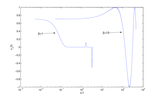
Figure 1: Comparison of the exact solution at $\beta=1$ and $\beta=10$ for $N=100$.

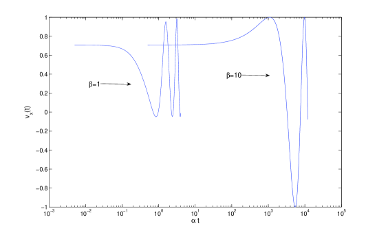
Figure 2: Comparison of the exact solution at $\beta=1$ and $\beta=10$ for $N=4$.

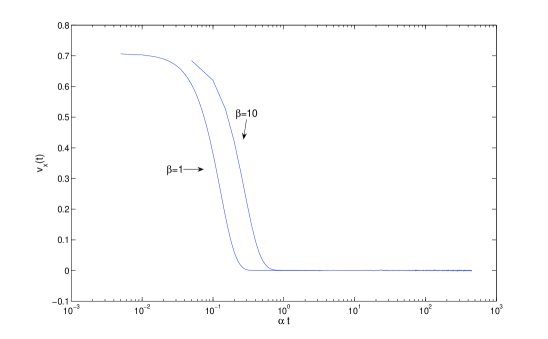
Figure 3: Comparison of the exact solution at $\beta=1$ and $\beta=10$ for $N=100$ for randomly generated $g_{n}$ and $\Omega_{n}$.

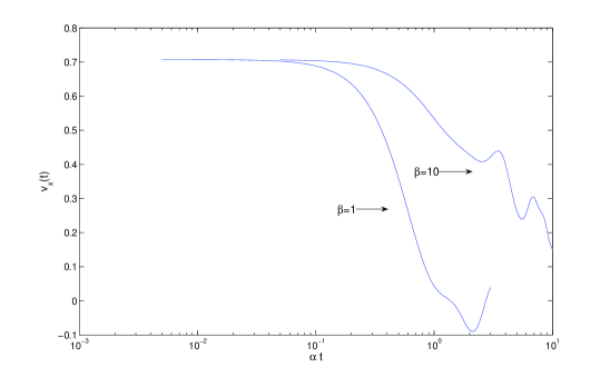
Figure 4: Comparison of the exact solution at $\beta=1$ and $\beta=10$ for $N=4$ for randomly generated $g_{n}$ and $\Omega_{n}$.

In the following, we plot the solutions of different orders of the NZ, TCL and PM master equations and compare them for the same parameter values.

4.4.2   NZ

In this subsection, we compare the solutions of different orders of the NZ master equation for $\Omega_{n}=g_{n}=1$. Fig. (5) shows the solutions to NZ2, NZ3, NZ4 and the exact solution for $\beta=1$ and $\beta=10$ up to the first recurrence time of the exact solution. For short times NZ4 is the better approximation. It can be seen that while NZ2 and NZ3 are bounded, NZ4 leaves the Bloch sphere. But note that the approximations under which these solutions have been obtained are valid for $\alpha t\ll 1$. The NZ4 solution leaves the Bloch sphere in a regime where the approximation is not valid. For $\beta=10$, NZ2 again has a periodic behavior (which is consistent with the solution), while the NZ3 and NZ4 solutions leave the Bloch sphere after small times. Fig. (6) shows the same graphs for $N=4$. In this case both NZ3 and NZ4 leave the Bloch sphere for $\beta=1$ and $\beta=10$, while NZ2 has a periodic behavior. A clear conclusion from these plots is that the NZ approximation is truly a short-time one: it becomes completely unreliable for times longer than $\alpha t\ll 1$.

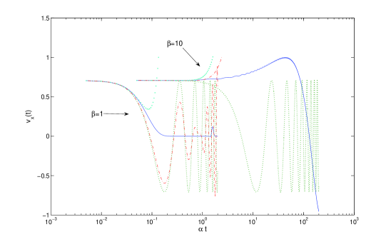
Figure 5: Comparison of the exact solution, NZ2, NZ3 and NZ4 at $\beta=1$ and $\beta=10$ for $N=100$. The exact solution is the solid (blue) line, NZ2 is the dashed (green) line, NZ3 is the dot-dashed (red) line and NZ4 is the dotted (cyan) line.

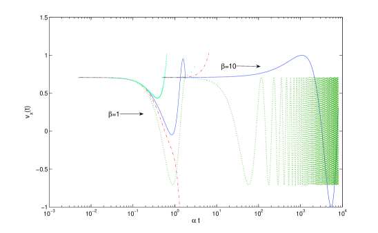
Figure 6: Comparison of the exact solution, NZ2, NZ3 and NZ4 at $\beta=1$ and $\beta=10$ for $N=4$. The exact solution is the solid (blue) line, NZ2 is the dashed (green) line, NZ3 is the dot-dashed (red) line and NZ4 is the dotted (cyan) line.

4.4.3   TCL

Fig. (7) plots the exact solution, TCL2, TCL3 and TCL4 at $\beta=1$ and $\beta=10$ for $N=100$ spins and $\Omega_{n}=g_{n}=1$. It can be seen that for $\beta=1$, the TCL solution approximates the exact solution well even for long times. However, the TCL solution cannot reproduce the recurrence behavior of the exact solution (also shown in the figure.) Fig. (8) shows the same graphs for $N=4$. In this case, while TCL2 and TCL3 decay, TCL4 increases exponentially and leaves the Bloch sphere after a short time. This is because the exponent in the solution of TCL4 in Eq. (4.3.2   NZ and TCL master equations) is positive. Here again the approximations under which the solutions have been obtained are valid only for small time scales and the graphs demonstrate the complete breakdown of the perturbation expansion for large values of $\alpha t$. Moreover, the graphs reveal the sensitivity of the approximation to temperature: the TCL fares much better at high temperatures.

In order to determine the validity of the TCL approximation, we look at the invertibility of the Kraus map derived in Eq. (164) or equivalently Eq. (171). As mentioned earlier, this map is non-invertible if $C(t)^{2}+S(t)^{2}=0$ for some $t$ (or equivalently $v_{x}(t)=0$ and $v_{y}(t)=0$). This will happen if and only if at least one of the $\beta_{n}$ is zero. This can occur when the bath density matrices of some of the bath spins are maximally mixed or in the limit of a very high bath temperature. Clearly, when the Kraus map is non-invertible, the TCL approach becomes invalid since it relies on the assumption that the information about the initial state is contained in the current state. This fact has also been observed for the spin-boson model with a damped Jaynes-Cummings Hamiltonian [30]. At the point where the Kraus map becomes non-invertible, the TCL solution deviates from the exact solution (see Fig.  9). We verified that both $v_{x}$ and $v_{y}$ vanish at this point.

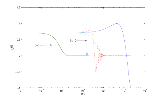
Figure 7: Comparison of the exact solution, TCL2, TCL3 and TCL4 at $\beta=1$ and $\beta=10$ for $N=100$. The exact solution is the solid (blue) line, TCL2 is the dashed (green) line, TCL3 is the dot-dashed (red) line and TCL4 is the dotted (cyan) line. Note that for $\beta=1$, the curves nearly coincide.

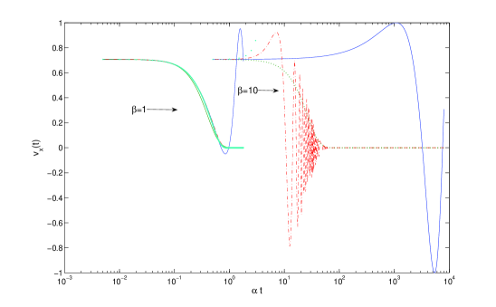
Figure 8: Comparison of the exact solution, TCL2, TCL3 and TCL4 at $\beta=1$ and $\beta=10$ for $N=4$. The exact solution is the solid (blue) line, TCL2 is the dashed (green) line, TCL3 is the dot-dashed (red) line and TCL4 is the dotted (cyan) line. Note that for $\beta=1$, TCL3, TCL4 and the exact solution nearly coincide.

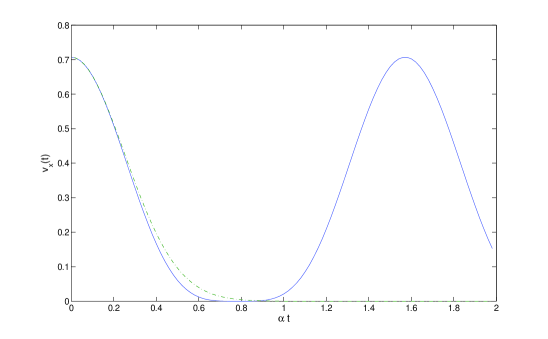
Figure 9: Comparison of TCL2 and the exact solution to demonstrate the validity of the TCL approximation for $N=4$ and $\beta=1$. The solid (blue) line denotes the exact solution and the dashed (green) line is TCL2. Note that the time axis here is on a linear scale. TCL2 breaks down at $\alpha t\approx 0.9$, where it remains flat, while the exact solution has a recurrence.

4.4.4   NZ, TCL, and PM

In this subsection, we compare the exact solution to TCL4, NZ4 and the solution of the optimal PM master equation. Fig. (10) shows these solutions for $N=100$ and $\beta=1$ and $\beta=10$ when $\Omega_{n}=g_{n}=1$. Here we observe that while the short-time behavior of the exact solution is approximated well by all the approximations we consider, the long-time behavior is approximated well only by PM.

For $\beta=1$, NZ4 leaves the Bloch sphere after a short time while TCL4 decays with the exact solution. But as before, the TCL solution cannot reproduce the recurrences seen in the exact solution. The optimal PM solution, by contrast, is capable of reproducing both the decay and the recurrences. TCL4 and NZ4 leave the Bloch sphere after a short time for $\beta=10$, while PM again reproduces the recurrences in the exact solution. Fig. 11 shows the corresponding graphs for $N=4$ and it can be seen that again PM can outperform both TCL and NZ for long times. Figs. 12 and 13 show the performance of TCL4, NZ4 and PM compared to the exact solution at a fixed time (for which the approximations are valid) for different temperatures ($\beta\in[0.01,10]$). It can be seen that both TCL4 and the optimal PM solution perform better than NZ4 at medium and high temperatures, with TCL4 outperforming PM at medium temperatures. The performance of NZ4 is enhanced at low temperatures, where it performs similarly to TCL4 (see also Figs. 10 and 11). This can be understood from the short-time approximation to the exact solution given in Eq. (183), which up to the precision for which it was derived is also an approximation of NZ2 [Eq. (192)]. As discussed above, this approximation (which also coincides with TCL2) is valid when $2Q_{2}(\alpha t)^{2}\ll 1$. As temperature decreases, so does the magnitude of $Q_{2}$, which leads to a better approximation at fixed $\alpha t$. Since NZ2 gives the lowest-order correction, this improvement is reflected in NZ4 as well.

In Figs. 14 and 15 we plot the averaged solutions over 50 ensembles of random values for $\Omega_{n}$ and $g_{n}$ in the interval $[-1,1]$. We see that on average TCL4, NZ4 and the optimal PM solution behave similarly to the case when $\Omega_{n}=g_{n}=1$. Due to the damping of the recurrences, especially when $N=100$, the TCL4 and the PM solutions match the exact solution closely for much longer times than in the deterministic case. Again, the PM solution is capable of qualitatively matching the behavior of the exact solution at long times.

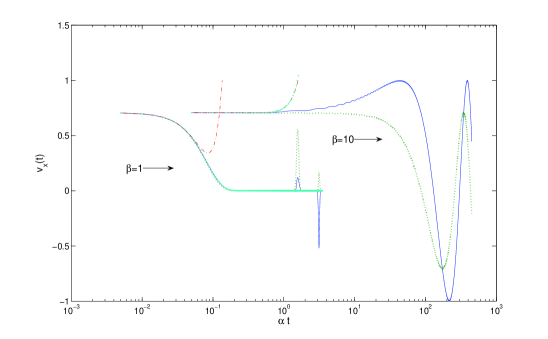
Figure 10: Comparison of the exact solution, NZ4, TCL4 and PM at $\beta=1$ and $\beta=10$ for $N=100$. The exact solution is the solid (blue) line, PM is the dashed (green) line, NZ4 is the dot-dashed (red) line and TCL4 is the dotted (cyan) line. Note that for $\beta=1$, TCL4, PM and the exact solution nearly coincide for short and medium times. Only PM captures the recurrences of the exact solution at long times.

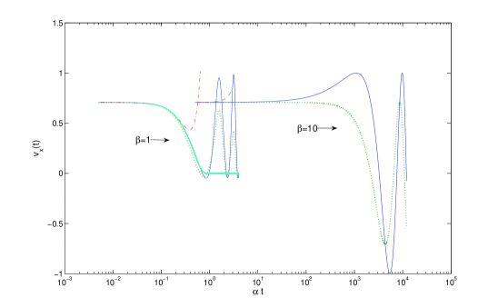
Figure 11: Comparison of the exact solution, NZ4, TCL4 and PM at $\beta=1$ and $\beta=10$ for $N=4$. The exact solution is the solid (blue) line, PM is the dashed (green) line, NZ4 is the dot-dashed (red) line and TCL4 is the dotted (cyan) line. Note that for $\beta=1$, TCL4 and the exact solution nearly coincide for short and medium times.

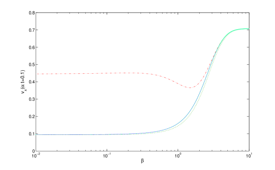
Figure 12: Comparison of the exact solution, NZ4, TCL4 and PM at $\alpha t=0.1$ for $N=100$ for different $\beta\in[0.01,10]$. The exact solution is the solid (blue) line, PM is the dashed (green) line, NZ4 is the dot-dashed (red) line and TCL4 is the dotted (cyan) line.

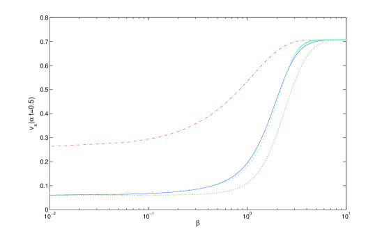
Figure 13: Comparison of the exact solution, NZ4, TCL4 and PM at $\alpha t=0.5$ for $N=4$ for different $\beta\in[0.01,10]$. The exact solution is the solid (blue) line, PM is the dashed (green) line, NZ4 is the dot-dashed (red) line and TCL4 is the dotted (cyan) line.

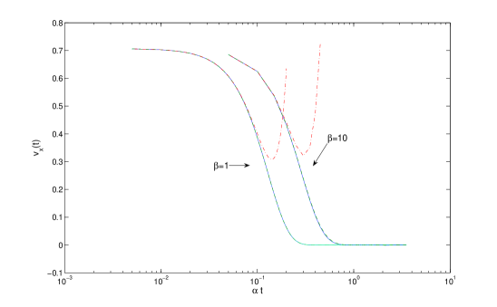
Figure 14: Comparison of the exact solution, NZ4, TCL4 and PM at $\beta=1$ and $\beta=10$ for $N=100$ for random values of $g_{n}$ and $\Omega_{n}$. The exact solution is the solid (blue) line, PM is the dashed (green) line, NZ4 is the dot-dashed (red) line and TCL4 is the dotted (cyan) line. Note that for $\beta=1$ and $\beta=10$, TCL4, PM and the exact solution nearly coincide.

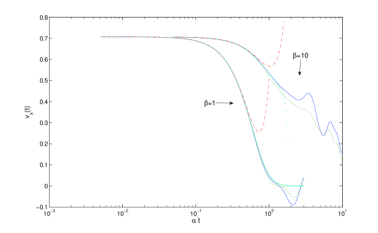
Figure 15: Comparison of the exact solution, NZ4, TCL4 and PM at $\beta=1$ and $\beta=10$ for $N=4$ for random values of $g_{n}$ and $\Omega_{n}$. The exact solution is the solid (blue) line, PM is the dashed (green) line, NZ4 is the dot-dashed (red) line and TCL4 is the dotted (cyan) line. Note that for $\beta=1$, TCL4, PM and the exact solution nearly coincide for short and medium times.

4.4.5   Coarse-graining approximation

Finally, we examine the coarse-graining approximation discussed in Section 4.3.1. We choose the time over which the average trace distance is calculated to be the time where the exact solution dies down. In Fig. 16 we plot the coarse-grained solution for the value of $\tau$ for which the trace distance to the exact solution is minimum. As can be seen, the coarse-graining approximation does not help since the Markovian assumption is not valid for this model. In deriving the coarse-graining approximation [104] one makes the assumption that the coarse-graining time scale is greater than any characteristic bath time scale. But the characteristic time scale of the bath is infinite in this case.

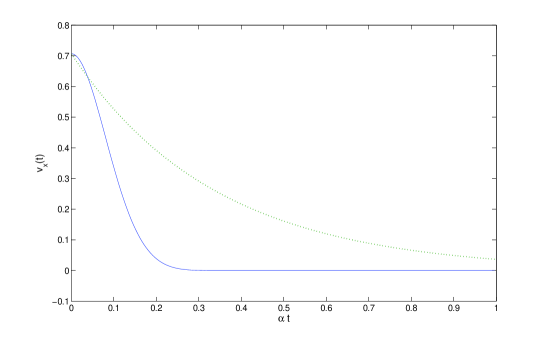
Figure 16: Comparison of the exact solution and the optimal coarse-graining approximation for $N=50$ and $\beta=1$. The exact solution is the solid (blue) line and the coarse-graining approximation is the dashed (green) line. Note the linear scale time axis.

4.5   Summary and conclusions

We studied the performance of various methods for approximating the evolution of an Ising model of an open quantum system for a qubit system coupled to a bath bath consisting of $N$ qubits. The high symmetry of the model allowed us to derive the exact dynamics of the system as well as find analytical solutions for the different master equations. We saw that the Markovian approximation fails for this model due to the time independence of the bath correlation functions. This is also reflected in the fact that the coarse-graining method [104] does not approximate the exact solution well. We discussed the performance of these solutions for various parameter regimes. Unlike other spin bath models discussed in literature (e.g., Ref. [29]), the odd-order bath correlation functions do not vanish, leading to the existence of odd-order terms in the solution of TCL and NZ equations. These terms describe the rotation around the $z$ axis of the Bloch sphere, a fact which is reflected in the exact solution. We showed that up to fourth order TCL performs better than NZ at medium and high temperatures. For low temperatures we demonstrated an enhancement in the performance of NZ and showed that NZ and TCL perform equally well. We showed that the TCL approach breaks down for certain parameter choices and related this to the non-invertibility of the Kraus map describing the system dynamics. We also studied the performance of the post-Markovian master equation obtained in [139] with an optimal memory kernel. We discussed possible ways of approximating the optimal kernel for short times and derived the kernel which leads to an exact fit to the NZ2 solution. It turns out that PM master equation performs as well as the TCL2 for a large number of spins and outperforms all orders of NZ and TCL considered here at long times, as it captures the recurrences of the exact solution.

Our study reveals the limitations of some of the best known master equations available in the literature, in the context of a spin bath. In general, perturbative approaches such as low-order NZ and TCL do well at short times (on a time scale set by the system-bath coupling constant) and fare very poorly at long times. These approximations are also very sensitive to temperature and do better in the high temperature limit. The PM does not do as well as TCL4 at short times but has the distinct advantage of retaining a qualitatively correct character for long times. This conclusion depends heavily on the proper choice of the memory kernel; indeed, when the memory kernel is not optimally chosen the PM can yield solutions which are not as satisfactory [109].

4.6   Appendix A: Bath correlation functions

Here we show how to calculate the bath correlation functions used in our simulations. The $k^{\mathrm{th}}$ order bath correlation function is defined as

$$Q_{k}=\mathrm{Tr}\{B^{k}\rho_{B}\},$$

where $B$ and $\rho_{B}$ were given in Eqs. (162) and (158), respectively. This yields:

$$Q_{k} = \mathrm{Tr}\{(\sum_{n}g_{n}\sigma_{n}^{z}-\theta I_{B})^{k}\sum_{l}\frac{\exp(-\beta E_{l})}{Z}|l\rangle\langle l|\}$$

$$= \sum_{l}\frac{\exp(-\beta E_{l})}{Z}\langle l|(\sum_{n}g_{n}\sigma_{n}^{z}-\theta I_{B})^{k}|l\rangle$$

$$= \sum_{l,l^{\prime},...,l^{\prime\prime\prime}}\frac{\exp(-\beta E_{l})}{Z}\langle l|(\sum_{n}g_{n}\sigma_{n}^{z}-\theta I_{B})|l^{\prime}\rangle\langle l^{\prime}|(\sum_{n^{\prime}}g_{n^{\prime}}\sigma_{n^{\prime}}^{z}-\theta I_{B})|l^{\prime\prime}\rangle\langle l^{\prime\prime}|\cdots$$

$$\cdots|l^{\prime\prime\prime}\rangle\langle l^{\prime\prime\prime}|(\sum_{n^{\prime\prime\prime}}g_{n^{\prime\prime\prime}}\sigma_{n^{\prime\prime\prime}}^{z}-\theta I_{B})|l\rangle$$

$$= \sum_{l,l^{\prime},...,l^{\prime\prime\prime}}\frac{\exp(-\beta E_{l})}{Z}(\sum_{n}g_{n}\langle l|\sigma_{n}^{z}|l^{\prime}\rangle-\theta)\delta_{ll^{\prime}}(\sum_{n^{\prime}}g_{n^{\prime}}\langle l^{\prime}|\sigma_{n^{\prime}}^{z}|l^{\prime\prime}\rangle-\theta)\delta_{l^{\prime}l^{\prime\prime}}\cdots$$

$$\cdots(\sum_{n^{\prime\prime\prime}}g_{n^{\prime\prime\prime}}\langle l^{\prime\prime\prime}|\sigma_{n^{\prime\prime\prime}}^{z}|l\rangle-\theta)\delta_{l^{\prime\prime\prime}l}$$

$$= \sum_{l}\frac{\exp(-\beta E_{l})}{Z}(\sum_{n}g_{n}\langle l|\sigma_{n}^{z}|l\rangle-\theta)(\sum_{n^{\prime}}g_{n^{\prime}}\langle l|\sigma_{n^{\prime}}^{z}|l\rangle-\theta)\cdots$$

$$\cdots(\sum_{n^{\prime\prime\prime}}g_{n^{\prime\prime\prime}}\langle l|\sigma_{n^{\prime\prime\prime}}^{z}|l\rangle-\theta)$$

$$= \sum_{l}\frac{\exp(-\beta E_{l})}{Z}(\sum_{n}g_{n}\langle l|\sigma_{n}^{z}|l\rangle-\theta)^{k},$$

or

$$Q_{k}=\frac{1}{Z}\sum_{l}(\tilde{E}_{l})^{k}\exp(-\beta E_{l}),$$ (233)

where $Z=\sum_{l}\exp(-\beta E_{l})$ and the expressions for $E_{l}$ and $\tilde{E}_{l}$ were given in Eqs. (167) and (169), respectively.

The above formulas are useful when the energy levels $E_{l}$ and $\tilde{E}_{l}$ are highly degenerate, which is the case for example when $g_{n}\equiv g$ and $\Omega_{n}\equiv\Omega$ for all $n$. For a general choice of these parameters, it is computationally more efficient to consider $\theta$ in the form (174) and the initial bath density matrix in the form (172). For example, the second order bath correlation function is

$$Q_{2} = \mathrm{Tr}\{(\sum_{m=1}^{N}g_{m}\sigma_{m}^{z}-\theta I)(\sum_{n=1}^{N}g_{n}\sigma_{n}^{z}-\theta I)\rho_{B}\}$$ (234)

$$= \mathrm{Tr}\{\sum_{n,m=1}^{N}g_{n}g_{m}\sigma_{n}^{z}\sigma_{m}^{z}\rho_{B}\}-2\theta\underbrace{\mathrm{Tr}\{\sum_{n=1}^{N}g_{n}\sigma_{n}^{z}\rho_{B}\}}_{\theta}+\theta^{2}$$

$$= \mathrm{Tr}\{\sum_{n,m=1}^{N}g_{n}g_{m}\sigma_{n}^{z}\sigma_{m}^{z}\bigotimes\limits_{n=1}^{N}\frac{1}{2}(I+\beta_{n}\sigma_{n}^{z})\}-\theta^{2}$$

$$= \sum_{n\neq m}^{N}\mathrm{Tr}\{g_{m}\frac{1}{2}(\sigma_{m}^{z}+\beta_{m}I)\}\mathrm{Tr}\{g_{n}\frac{1}{2}(\sigma_{n}^{z}+\beta_{n}I)\}\prod\limits_{j\neq m,n}\mathrm{Tr}\{\frac{1}{2}(I+\beta_{j}\sigma_{j}^{z})\}$$

$$+\mathrm{Tr}\{\sum_{n=1}^{N}g_{n}^{2}\rho_{B}\}-\theta^{2}$$

$$= \underbrace{\sum_{n,m=1}^{N}g_{m}\beta_{m}g_{n}\beta_{n}}_{\theta^{2}}-\sum_{n=1}^{N}g_{n}^{2}\beta_{n}^{2}+\sum_{n=1}^{N}g_{n}^{2}-\theta^{2}$$

$$= \sum_{n=1}^{N}g_{n}^{2}(1-\beta_{n}^{2}).$$

Using the identity $1-\tanh^{2}(-x/2)=2/(1+\cosh x)$, this correlation function can be expressed in terms of the bath spectral density function [Eq. (159)] as follows:

$$Q_{2} = \sum_{n=1}^{N}g_{n}^{2}(1-\beta_{n}^{2})$$

$$= \int_{-\infty}^{\infty}\delta(\Omega-\Omega_{n})|g_{n}|^{2}(1-\tanh^{2}(-\frac{\Omega}{2kT}))\mathrm{d}\Omega$$

$$= \int_{-\infty}^{\infty}\frac{2J(\Omega)\mathrm{d}\Omega}{1+\cosh(\frac{\Omega}{kT})}.$$

Higher order correlation functions are computed analogously.

4.7   Appendix B: Cumulants for the NZ and TCL master equations

We calculate the explicit expressions for the cumulants appearing in Eq. (215), needed to find the NZ and TCL perturbation expansions up to fourth order.

Second order:

$$\langle\mathcal{L}^{2}\rangle\rho = -\mathrm{Tr}_{B}\{[H_{I},[H_{I},\rho]]\}\otimes\rho_{B}$$ (235)

$$= -\mathrm{Tr}_{B}\{H_{I}^{2}\rho-2H_{I}\rho H_{I}+\rho H_{I}^{2}\}\otimes\rho_{B}$$

$$= -2Q_{2}(\rho_{S}-\sigma_{z}\rho_{S}\sigma_{z})\otimes\rho_{B}$$

$$\equiv \rho^{\prime},$$

$$\langle\mathcal{L}^{2}\rangle^{2}\rho = \mathcal{P}\mathcal{L}^{2}\mathcal{P}\mathcal{P}\mathcal{L}^{2}\mathcal{P}\rho$$

$$= \mathcal{P}\mathcal{L}^{2}\mathcal{P}\rho^{\prime}$$

$$= -2Q_{2}(\rho_{S}^{\prime}-\sigma_{z}\rho_{S}^{\prime}\sigma_{z})\otimes\rho_{B},$$

where $\rho_{S}^{\prime}=\mathrm{Tr}_{B}{\rho}^{\prime}=-2Q_{2}(\rho_{S}-\sigma_{z}\rho_{S}\sigma_{z})$. Therefore

$$\langle\mathcal{L}^{2}\rangle^{2}\rho = -2Q_{2}\{(-2Q_{2}(\rho_{S}-\sigma_{z}\rho_{S}\sigma_{z}))-\sigma_{z}(-2Q_{2}(\rho_{S}-\sigma_{z}\rho_{S}\sigma_{z}))\sigma_{z}\}\otimes\rho_{B}$$ (236)

$$= 8Q_{2}^{2}(\rho_{S}-\sigma_{z}\rho_{S}\sigma_{z})\otimes\rho_{B}.$$

Third order:

$$\langle\mathcal{L}^{3}\rangle\rho = i\mathrm{Tr}_{B}\{[H_{I},[H_{I},[H_{I},\rho]]]\}\otimes\rho_{B}$$ (237)

$$= i\mathrm{Tr}_{B}\{H_{I}^{3}\rho-3H_{I}^{2}\rho H_{I}+3H_{I}\rho H_{I}^{2}-\rho H_{I}^{3}\}\otimes\rho_{B}$$

$$= 4iQ_{3}(\sigma_{z}\rho_{S}-\rho_{S}\sigma_{z})\otimes\rho_{B}.$$

Fourth order:

$$\langle\mathcal{L}^{4}\rangle\rho = \mathrm{Tr}_{B}\{[H_{I},[H_{I},[H_{I},[H_{I},\rho]]]]\}\otimes\rho_{B}$$ (238)

$$= \mathrm{Tr}_{B}\{H_{I}^{4}\rho-4H_{I}^{3}\rho H_{I}+6H_{I}^{2}\rho H_{I}^{2}-4H_{I}\rho H_{I}^{3}+\rho H_{I}^{4}\}\otimes\rho_{B}$$

$$= 8Q_{4}(\rho_{S}-\sigma_{z}\rho_{S}\sigma_{z})\otimes\rho_{B}.$$

Chapter 5:   Continuous quantum error correction for non-Markovian decoherence

In this chapter we continue our exploration of non-Markovian decoherence. This time, we compare Markovian and non-Markovian error models in light of the performance of continuous quantum error correction. We consider again an Ising decoherence model of the type we studied in the previous chapter, but in a much simpler version—when the environment consists of only a single qubit. This allows us to solve exactly the evolution of a multi-qubit code in which each qubit is coupled to an independent bath when the code is subject to continuous error correction. The conclusions we obtain, however, extend beyond this model and apply for general non-Markovian decoherence.

5.1   Preliminaries

5.1.1   Continuous quantum error correction

In general, error probabilities increase with time. No matter how complicated a code or how many levels of concatenation are involved, the probability of uncorrectable errors is never truly zero, and if the system is exposed to noise for a sufficiently long time, the weight of uncorrectable errors can accumulate. To combat this, error correction must be applied repeatedly and sufficiently often. If one assumes that the time for an error-correcting operation is small compared to other relevant time scales of the system, error-correcting operations can be considered instantaneous. Then the scenario of repeated error correction leads to a discrete evolution which often may be difficult to describe. To study the evolution of a system in the limit of frequently applied instantaneous error correction, Paz and Zurek proposed to describe error correction as a continuous quantum jump process [125]. In this model, the infinitesimal error-correcting transformation that the density matrix of the encoded system undergoes during a time step $dt$ is

$$\rho\rightarrow(1-\kappa dt)\rho+\kappa dt\Phi(\rho),$$ (239)

where $\Phi(\rho)$ is the completely positive trace-preserving (CPTP) map describing a full error-correcting operation, and $\kappa$ is the error-correction rate. The full error-correcting operation $\Phi(\rho)$ consists of a syndrome detection, followed (if necessary) by a unitary correction operation conditioned on the syndrome.

Consider, for example, the three-qubit bit-flip code whose purpose is to protect an unknown qubit state from bit-flip (Pauli $X$) errors. The code space is spanned by $|\overline{0}\rangle=|000\rangle$ and $|\overline{1}\rangle=|111\rangle$, and the stabilizer generators are $ZZI$ and $IZZ$ (see Section 8.3). Here by $X=\sigma^{x}$, $Y=\sigma^{y}$, $Z=\sigma^{z}$ and $I$ we denote the usual Pauli operators and the identity, respectively, and a string of three operators represents the tensor product of operators on each of the three qubits. The standard error-correction procedure involves a measurement of the stabilizer generators, which projects the state onto one of the subspaces spanned by $|000\rangle$ and $|111\rangle$, $|100\rangle$ and $|011\rangle$, $|010\rangle$ and $|101\rangle$, or $|001\rangle$ and $|110\rangle$; the outcome of these measurements is the error syndrome. Assuming that the probability for two- or three-qubit errors is negligible, then with high probability the result of this measurement is either the original state with no errors, or with a single $X$ error on the first, the second, or the third qubit. Depending on the outcome, one then applies an $X$ gate to the erroneous qubit and transforms the state back to the original one. The CPTP map $\Phi(\rho)$ for this code can be written explicitly as

$$\begin{split}\Phi(\rho)=\left(|000\rangle\langle 000|+|111\rangle\langle 111|\right)\rho\left(|000\rangle\langle 000|+|111\rangle\langle 111|\right)\\ +\left(|000\rangle\langle 100|+|111\rangle\langle 011|\right)\rho\left(|100\rangle\langle 000|+|011\rangle\langle 111|\right)\\ +\left(|000\rangle\langle 010|+|111\rangle\langle 101|\right)\rho\left(|010\rangle\langle 000|+|101\rangle\langle 111|\right)\\ +\left(|000\rangle\langle 001|+|111\rangle\langle 110|\right)\rho\left(|001\rangle\langle 000|+|110\rangle\langle 111|\right).\end{split}$$ (240)

The quantum-jump process (239) can be viewed as a smoothed version of the discrete scenario of repeated error correction, in which instantaneous full error-correcting operations are applied at random times with rate $\kappa$. It can also be looked upon as arising from a continuous sequence of infinitesimal CPTP maps of the type (239). In practice, such a weak map is never truly infinitesimal, but rather has the form

$$\rho\rightarrow(1-\epsilon^{2})\rho+\epsilon^{2}\Phi(\rho),$$ (241)

where $\epsilon\ll 1$ is a small but finite parameter, and the weak operation takes a small but nonzero time $\tau_{c}$. For times $t$ much greater than $\tau_{c}$ ($\tau_{c}\ll t$), the weak error-correcting map (241) is well approximated by the infinitesimal form (239), where the rate of error correction is

$$\kappa=\epsilon^{2}/\tau_{c}.$$ (242)

A weak map of the form (241) could be implemented, for example, by a weak coupling between the system and an ancilla via an appropriate Hamiltonian, followed by discarding the ancilla. A closely related scenario, where the ancilla is continuously cooled in order to reset it to its initial state, was studied in [136].

Another way of implementing the weak map (241) is via weak measurements followed by weak unitaries dependent on the outcome. In the appendix at the end of this chapter, we give an example of such an implementation for the case of the bit-flip code—when $\Phi(\rho)$ is given by (240). We also present a scheme in terms of weak measurements for codes that correct arbitrary single-qubit errors. In the latter case, the resulting weak map is not the same as (241), but also yields the strong error-correcting map $\Phi(\rho)$ when exponentiated. We point out that the weak measurements used in these schemes are not weak versions of the strong measurements for syndrome detection—they are in a different basis. They can be regarded as weak versions of a different set of strong measurements which, when followed by an appropriate unitary, yield the same map $\Phi(\rho)$ on average. Thus, the workings of continuous error correction, when it is driven by weak measurements, does not translate directly into the error syndrome detection and correction of the standard paradigm. In this sense, the continuous approach can be regarded as a different paradigm for error correction—one based on weak measurements and weak unitary operations. The idea of using continuous weak measurements and unitary operations for error correction has been explored in the context of different heuristic schemes [7, 135], some of which are based on a direct “continuization” of the syndrome measurements. In this study we consider continuous error correction of the type given by Eq. (239).

5.1.2   Markovian decoherence

So far, continuous quantum error correction has been studied only for Markovian error models. As we discussed in the previous chapter, the Markovian approximation describes situations where the bath-correlation times are much shorter than any characteristic time scale of the system [30]. In this limit, the dynamics can be described by a semi-group master equation in the Lindblad form [106]:

$$\frac{d\rho}{dt}=L(\rho)\equiv-i[H,\rho]+\frac{1}{2}\underset{j}{\sum}\lambda_{j}(2L_{j}\rho L_{j}^{\dagger}-L_{j}^{\dagger}L_{j}\rho-\rho L_{j}^{\dagger}L_{j}).$$ (243)

Here $H$ is the system Hamiltonian and the $\{L_{j}\}$ are suitably normalized Lindblad operators describing different error channels with decoherence rates $\lambda_{j}$. For example, the Liouvillian

$$L(\rho)=\underset{j}{\sum}\lambda_{j}(X_{j}\rho X_{j}-\rho),$$ (244)

where $X_{j}$ denotes a local bit-flip operator acting on the $j$-th qubit, describes independent Markovian bit-flip errors.

For a system undergoing Markovian decoherence and error correction of the type (239), the evolution is given by the equation

$$\frac{d\rho}{dt}=L(\rho)+\kappa\Gamma(\rho),$$ (245)

where $\Gamma(\rho)=\Phi(\rho)-\rho$. In [125], Paz and Zurek showed that if the set of errors $\{L_{j}\}$ are correctable by the code, in the limit of infinite error-correction rate (strong error-correcting operations applied continuously often) the state of the system freezes and is protected from errors at all times. The effect of freezing can be understood by noticing that the transformation arising from decoherence during a short time step $\Delta t$, is

$$\rho\rightarrow\rho+L(\rho)\Delta t+\textit{O}(\Delta t^{2}),$$ (246)

i.e., the weight of correctable errors emerging during this time interval is proportional to $\Delta t$, whereas uncorrectable errors (e.g., multi-qubit bit flips in the case of the three-qubit bit-flip code) are of order $\textit{O}(\Delta t^{2})$. Thus, if errors are constantly corrected, in the limit $\Delta t\rightarrow 0$ uncorrectable errors cannot accumulate, and the evolution stops.

5.1.3   The Zeno effect. Error correction versus error prevention

The effect of “freezing” in continuous error correction strongly resembles the quantum Zeno effect [111], in which frequent measurements slow down the evolution of a system, freezing the state in the limit where they are applied continuously. The Zeno effect arises when the system and its environment are initially decoupled and they undergo a Hamiltonian-driven evolution, which leads to a quadratic change with time of the state during the initial moments [113] (the so called Zeno regime). Let the initial state of the system plus the bath be $\rho_{SB}(0)=|0\rangle\langle 0|_{S}\otimes\rho_{B}(0)$. For small times, the fidelity of the system’s density matrix with the initial state $\alpha(t)=\textrm{Tr}\left\{\left(|0\rangle\langle 0|_{S}\otimes I_{B}\right)\rho_{SB}(t)\right\}$ can be approximated as

$$\alpha(t)=1-Ct^{2}+\textit{O}(t^{3}).$$ (247)

In terms of the Hamiltonian $H_{SB}$ acting on the entire system, the coefficient $C$ is

$$C=\textrm{Tr}\left\{H_{SB}^{2}\left(|0\rangle\langle 0|_{S}\otimes\rho_{B}(0)\right)\right\}-\textrm{Tr}\left\{H_{SB}\left(|0\rangle\langle 0|_{S}\otimes I_{B}\right)H_{SB}\left(|0\rangle\langle 0|_{S}\otimes\rho_{B}(0)\right)\right\}.$$ (248)

According to Eq. (247), if after a short time step $\Delta t$ the system is measured in an orthogonal basis which includes the initial state $|0\rangle$, the probability to find the system in a state other than the initial state is of order $\textit{O}(\Delta t^{2})$. Thus if the state is continuously measured ($\Delta t\rightarrow 0$), this prevents the system from evolving.

It has been proposed to utilize the quantum Zeno effect in schemes for error prevention [180, 15, 158], in which an unknown encoded state is prevented from errors simply by frequent measurements which keep it inside the code space. The approach is similar to error correction in that the errors for which the code is designed send a codeword to a space orthogonal to the code space. The difference is that different errors need not be distinguishable, since the procedure does not involve correction of errors, but their prevention. In [158] it was shown that with this approach it is possible to use codes of smaller redundancy than those needed for error correction and a four-qubit encoding of a qubit was proposed, which is capable of preventing arbitrary independent errors arising from Hamiltonian interactions. The possibility of this approach implicitly assumes the existence of a Zeno regime, and fails if we assume Markovian decoherence for all times. This is because the probability of errors emerging during a time step $dt$ in a Markovian model is proportional to $dt$ (rather than $dt^{2}$), and hence errors will accumulate with time if not corrected.

From the above observations we see that error correction is capable of achieving results in noise regimes where error prevention fails. Of course, this advantage is at the expense of a more complicated procedure—in addition to the measurements used in error prevention, error correction involves unitary correction operations, and in general requires codes with higher redundancy. At the same time, we see that in the Zeno regime it is possible to reduce decoherence using weaker resources than those needed in the case of Markovian noise. This suggests that in this regime error correction may exhibit higher performance than it does for Markovian decoherence.

5.1.4   Non-Markovian decoherence

Markovian decoherence is an approximation valid for times much larger than the memory of the environment. As we saw in the previous chapter, however, in many situations of practical significance the memory of the environment cannot be neglected and the evolution is highly non-Markovian. Furthermore, no evolution is strictly Markovian, and for a system initially decoupled from its environment a Zeno regime is always present, short though it may be [113]. If the time resolution of error-correcting operations is high enough so that they “see” the Zeno regime, this could give rise to different behavior.

The existence of a Zeno regime is not the only interesting feature of non-Markovian decoherence. The mechanism by which errors accumulate in a general Hamiltonian interaction with the environment may differ significantly from the Markovian case, since the system may develop nontrivial correlations with the environment. For example, imagine that some time after the initial encoding of a system, a strong error-correcting operation is applied. This brings the state inside the code space, but the state contains a nonzero portion of errors non-distinguishable by the code. Thus the new state is mixed and is generally correlated with the environment. A subsequent error-correcting operation can only aim at correcting errors arising after this point, since the errors already present inside the code space are in principle uncorrectable. Subsequent errors on the density matrix, however, may not be completely positive due to the correlations with the environment.

Nevertheless, it follows from a result in [141] that an error-correction procedure which is capable of correcting a certain class of completely positive (CP) maps, can also correct any linear noise map whose operator elements can be expressed as linear combinations of the operator elements in a correctable CP map. This implies, in particular, that an error-correction procedure that can correct arbitrary single-qubit CP maps can correct arbitrary single-qubit linear maps. In this context, we note that the effects of system-environment correlations in non-Markovian error models have also been studied from the perspective of fault tolerance, and it has been shown that the threshold theorem can be extended to various types of non-Markovian noise [156, 12, 3].

Another important difference from the Markovian case is that error correction and the effective noise on the reduced density matrix of the system cannot be treated as independent processes. One could derive an equation for the effective evolution of the system alone subject to interaction with the environment, like the Nakajima-Zwanzig [112, 181] or the time-convolutionless (TCL) [143, 142] master equations, but the generator of transformations at a given moment in general will depend (implicitly or explicitly) on the entire history up to this moment. Therefore, adding error correction can nontrivially affect the effective error model. This means that in studying the performance of continuous error correction one either has to derive an equation for the effective evolution of the encoded system, taking into account error correction from the very beginning, or one has to look at the evolution of the entire system—including the bath—where the error generator and the generator of error correction can be considered independent. In the latter case, for sufficiently small $\tau_{c}$, the evolution of the entire system including the bath can be described by

$$\frac{d\rho}{dt}=-i[H,\rho]+\kappa\Gamma(\rho),$$ (249)

where $\rho$ is the density matrix of the system plus bath, $H$ is the total Hamiltonian, and the error-correction generator $\Gamma$ acts locally on the encoded system. In this study, we take this approach for a sufficiently simple bath model which allows us to find a solution for the evolution of the entire system.

5.1.5   Plan of this chapter

The rest of the chapter is organized as follows. To develop understanding of the workings of continuous error correction, in Section 5.2 we look at a simple example: an error-correction code consisting of only one qubit which aims at protecting a known state. We discuss the difference in performance for Markovian and non-Markovian decoherence, and argue the implications it has for the case of multi-qubit codes. In Section 5.3, we study the three-qubit bit-flip code. We first review the performance of continuous error correction in the case of Markovian bit-flip decoherence, which was first studied in [125]. We then consider a non-Markovian model, where each qubit in the code is coupled to an independent bath qubit. This model is a simple version of the one studied in the previous chapter, and it allows us to solve for its evolution analytically. In the limit of large error-correction rates, the effective evolution approaches the evolution of a single qubit without error correction, but the coupling strength is now decreased by a factor which scales quadratically with the error-correction rate. This is opposed to the case of Markovian decoherence, where the same factor scales linearly with the rate of error-correction. In Section 5.4, we show that the quadratic enhancement in the performance over the case of Markovian noise can be attributed to the presence of a Zeno regime and argue that for general stabilizer codes and independent errors, the performance of continuous error correction would exhibit the same qualitative characteristics. In Section 5.5, we conclude. In the Appendix (Section 5.6), we present an implementation of the quantum-jump error correcting model that uses weak measurements and weak unitary operations.

5.2   The single-qubit code

Consider the problem of protecting a qubit in state $|0\rangle$ from bit-flip errors. This problem can be regarded as a trivial example of a stabilizer code, where the code space is spanned by $|0\rangle$ and its stabilizer is $Z$. Let us consider the Markovian bit-flip model first. The evolution of the state subject to bit-flip errors and error correction is described by Eq. (245) with

$$L(\rho)=\lambda(X\rho X-\rho),$$ (250)

and

$$\Gamma(\rho)=|0\rangle\langle 0|\rho|0\rangle\langle 0|+|0\rangle\langle 1|\rho|1\rangle\langle 0|-\rho.$$ (251)

If the state lies on the z-axis of the Bloch sphere, it will never leave it, since both the noise generator (250) and the error-correction generator (251) keep it on the axis. We will take the qubit to be initially in the desired state $|0\rangle$, and therefore at any later moment it will have the form $\rho(t)=\alpha(t)|0\rangle\langle 0|+(1-\alpha(t))|1\rangle\langle 1|$, $\alpha(t)\in[0,1]$. The coefficient $\alpha(t)$ has the interpretation of a fidelity with the trivial code space spanned by $|0\rangle$. For an infinitesimal time step $dt$, the effect of the noise is to decrease $\alpha(t)$ by the amount $\lambda(2\alpha(t)-1)dt$ and that of the correcting operation is to increase it by $\kappa(1-\alpha(t))dt$. The net evolution is then described by

$$\frac{d\alpha(t)}{dt}=-(\kappa+2\lambda)\alpha(t)+(\kappa+\lambda).$$ (252)

The solution is

$$\alpha(t)=(1-\alpha_{*}^{\rm M})e^{-(\kappa+2\lambda)t}+\alpha_{*}^{\rm M},$$ (253)

where

$$\alpha_{*}^{\rm M}=1-\frac{1}{2+r},$$ (254)

and $r=\kappa/\lambda$ is the ratio between the rate of error correction and the rate of decoherence. We see that the fidelity decays, but it is confined above its asymptotic value $\alpha_{*}^{\rm M}$, which can be made arbitrarily close to 1 for a sufficiently large $r$.

Now let us consider a non-Markovian error model. We choose the simple scenario where the system is coupled to a single bath qubit via the Hamiltonian

$$H=\gamma X\otimes X,$$ (255)

where $\gamma$ is the coupling strength. This is the Ising Hamiltonian (147) for the case of a single bath qubit, but in the basis $|+\rangle=\frac{|0\rangle+|1\rangle}{\sqrt{2}}$, $|-\rangle=\frac{|0\rangle-|1\rangle}{\sqrt{2}}$. As we noted in Chapter 4 (Section 4.1), the model of a single bath qubit can be a good approximation for situations in which the coupling to a single spin from the bath dominates over other interactions.

We will assume that the bath qubit is initially in the maximally mixed state, which can be thought of as an equilibrium state at high temperature. From Eq. (249) one can verify that if the system is initially in the state $|0\rangle$, the state of the system plus the bath at any moment will have the form

$$\rho(t)=\left(\alpha(t)|0\rangle\langle 0|+(1-\alpha(t))|1\rangle\langle 1|\right)\otimes\frac{I}{2}-\beta(t)Y\otimes\frac{X}{2}.$$ (256)

In the tensor product, the first operator belongs to the Hilbert space of the system and the second to the Hilbert space of the bath. We have $\alpha(t)\in[0,1]$, and $|\beta(t)|\leq\sqrt{\alpha(t)(1-\alpha(t))},\beta(t)\in R$. The reduced density matrix of the system has the same form as the one for the Markovian case. The traceless term proportional to $\beta(t)$ can be thought of as a “hidden” part, which nevertheless plays an important role in the error-creation process, since errors can be thought of as being transferred to the “visible” part from the “hidden” part (and vice versa). This can be seen from the fact that during an infinitesimal time step $dt$, the Hamiltonian changes the parameters $\alpha$ and $\beta$ as follows:

$$\alpha\rightarrow\alpha-2\beta\gamma dt,$$

$$\beta\rightarrow\beta+(2\alpha-1)\gamma dt.$$ (257)

The effect of an infinitesimal error-correcting operation is

$$\alpha\rightarrow\alpha+(1-\alpha)\kappa dt,$$

$$\beta\rightarrow\beta-\beta\kappa dt.$$ (258)

Note that the hidden part is also being acted upon. Putting it all together, we get the system of equations

$$\frac{d\alpha(t)}{dt}=\kappa(1-\alpha(t))-2\gamma\beta(t),$$

$$\frac{d\beta(t)}{dt}=\gamma(2\alpha-1)-\kappa\beta(t).$$ (259)

The solution for the fidelity $\alpha(t)$ is

$$\alpha(t)=\frac{2\gamma^{2}+\kappa^{2}}{4\gamma^{2}+\kappa^{2}}+e^{-\kappa t}\left(\frac{\kappa\gamma}{4\gamma^{2}+\kappa^{2}}\sin{2\gamma t}+\frac{2\gamma^{2}}{4\gamma^{2}+\kappa^{2}}\cos{2\gamma t}\right).$$ (260)

We see that as time increases, the fidelity stabilizes at the value

$$\alpha_{*}^{\rm NM}=\frac{2+R^{2}}{4+R^{2}}=1-\frac{2}{4+R^{2}},$$ (261)

where $R=\kappa/\gamma$ is the ratio between the error-correction rate and the coupling strength. In Fig. 1 we have plotted the fidelity as a function of the dimensionless parameter $\gamma t$ for three different values of $R$. For error-correction rates comparable to the coupling strength ($R=1$), the fidelity undergoes a few partial recurrences before it stabilizes close to $\alpha_{*}^{\rm NM}$. For larger $R=2$, however, the oscillations are already heavily damped and for $R=5$ the fidelity seems confined above $\alpha_{*}^{\rm NM}$. As $R$ increases, the evolution becomes closer to a decay like the one in the Markovian case.

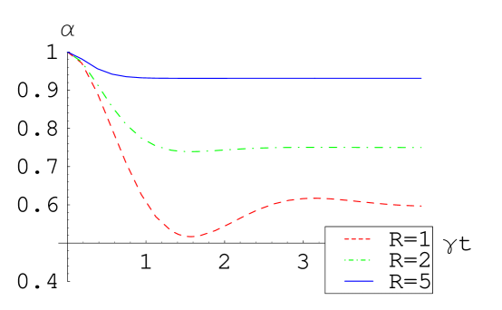
Figure 17: Fidelity of the single-qubit code with continuous bit-flip errors and error correction, as a function of dimensionless time $\gamma t$, for three different values of the ratio $R=\kappa/\gamma$.

A remarkable difference, however, is that the asymptotic weight outside the code space ($1-\alpha_{*}^{\rm NM}$) decreases with $\kappa$ as $1/\kappa^{2}$, whereas in the Markovian case the same quantity decreases as $1/\kappa$. The asymptotic value can be obtained as an equilibrium point at which the infinitesimal weight flowing out of the code space during a time step $dt$ is equal to the weight flowing into it. The latter corresponds to vanishing right-hand sides in Eqs. (252) and (259). In Section 5.4, we will show that the difference in the equilibrium code-space fidelity for the two different types of decoherence arises from the difference in the corresponding evolutions during initial times.

For multi-qubit codes, error correction cannot preserve a high fidelity with the initial codeword for all times, because there will be multi-qubit errors that can lead to errors within the code space itself. But it is natural to expect that the code-space fidelity can be kept above a certain value, since the effect of the error-correcting map (239) is to oppose its decrease. If similarly to the single-qubit code there is a quadratic difference in the code-space fidelity for the cases of Markovian and non-Markovian decoherence, this could lead to a different performance of the error-correction scheme with respect to the rate of accumulation of uncorrectable errors inside the code space. This is because multi-qubit errors that can lead to transformations entirely within the code space during a time step $dt$ are of order $\textit{O}(dt^{2})$. This means that if the state is kept constantly inside the code space (as in the limit of an infinite error-correction rate), uncorrectable errors will never develop. But if there is a finite nonzero portion of correctable errors, by the error mechanism it will give rise to errors not distinguishable or misinterpreted by the code. Therefore, the weight outside the code space can be thought of as responsible for the accumulation of uncorrectable errors, and consequently a difference in its magnitude may lead to a difference in the overall performance. In the following sections we will see that this is indeed the case.

5.3   The three-qubit bit-flip code

5.3.1   A Markovian error model

Even though the three-qubit bit-flip code can correct only bit-flip errors, it captures most of the important characteristics of nontrivial stabilizer codes. Before we look at a non-Markovian model, we will review the Markovian case which was studied in [125]. Let the system decohere through identical independent bit-flip channels, i.e., $L(\rho)$ is of the form (244) with $\lambda_{1}=\lambda_{2}=\lambda_{3}=\lambda$. Then one can verify that the density matrix at any moment can be written as

$$\rho(t)=a(t)\rho(0)+b(t)\rho_{1}+c(t)\rho_{2}+d(t)\rho_{3},$$ (262)

where

$$\rho_{1}=\frac{1}{3}(X_{1}\rho(0)X_{1}+X_{2}\rho(0)X_{2}+X_{3}\rho(0)X_{3}),$$

$$\rho_{2}=\frac{1}{3}(X_{1}X_{2}\rho(0)X_{1}X_{2}+X_{2}X_{3}\rho(0)X_{2}X_{3}+X_{1}X_{3}\rho(0)X_{1}X_{3}),$$ (263)

$$\rho_{3}=X_{1}X_{2}X_{3}\rho(0)X_{1}X_{2}X_{3},$$

are equally-weighted mixtures of single-qubit, two-qubit and three-qubit errors on the original state.

The effect of decoherence for a single time step $dt$ is equivalent to the following transformation of the coefficients in Eq. (262):

$$\begin{split}a\rightarrow a-3a\lambda dt+b\lambda dt,\\ b\rightarrow b+3a\lambda dt-3b\lambda dt+2c\lambda dt,\\ c\rightarrow c+2b\lambda dt-3c\lambda dt+3d\lambda dt,\\ d\rightarrow d+c\lambda dt-3d\lambda dt.\end{split}$$ (264)

If the system is initially inside the code space, combining Eq. (264) with the effect of the weak error-correcting map $\rho\rightarrow(1-\kappa dt)\rho+\kappa dt\Phi(\rho)$, where $\Phi(\rho)$ is given in Eq. (240), yields the following system of first-order linear differential equations for the evolution of the system subject to decoherence plus error correction:

$$\begin{split}\frac{da(t)}{dt}=-3\lambda a(t)+(\lambda+\kappa)b(t),\\ \frac{db(t)}{dt}=3\lambda a(t)-(3\lambda+\kappa)b(t)+2\lambda c(t),\\ \frac{dc(t)}{dt}=2\lambda b(t)-(3\lambda+\kappa)c(t)+3\lambda d(t),\\ \frac{dd(t)}{dt}=(\lambda+\kappa)c(t)-3\lambda d(t).\end{split}$$ (265)

The exact solution has been found in [125]. Here we just note that for the initial conditions $a(0)=1,b(0)=c(0)=d(0)=0$, the exact solution for the weight outside the code space is

$$b(t)+c(t)=\frac{3}{4+r}(1-e^{-(4+r)\lambda t}),$$ (266)

where $r=\kappa/\lambda$. We see that similarly to what we obtained for the trivial code in the previous section, the weight outside the code space quickly decays to its asymptotic value $\frac{3}{4+r}$ which scales as $1/r$. But note that here the asymptotic value is roughly three times greater than that for the single-qubit model. This corresponds to the fact that there are three single-qubit channels. More precisely, it can be verified that if for a given $\kappa$ the uncorrected weight by the single-qubit scheme is small, then the uncorrected weight by a multi-qubit code using the same $\kappa$ and the same kind of decoherence for each qubit scales approximately linearly with the number of qubits. Similarly, the ratio $r$ required to preserve a given overlap with the code space scales linearly with the number of qubits in the code.

The most important difference from the single-qubit model is that in this model there are uncorrectable errors that cause a decay of the state’s fidelity inside the code space. Due to the finiteness of the resources employed by our scheme, there always remains a nonzero portion of the state outside the code space, which gives rise to uncorrectable three-qubit errors. To understand how the state decays inside the code space, we ignore the terms of the order of the weight outside the code space in the exact solution. We obtain:

$$a(t)\approx\frac{1+e^{-\frac{6}{r}2\lambda t}}{2}\approx 1-d(t),$$ (267)

$$b(t)\approx c(t)\approx 0.$$ (268)

Comparing this solution to the expression for the fidelity of a single decaying qubit without error correction—which can be seen from Eq. (253) for $\kappa=0$—we see that the encoded qubit decays roughly as if subject to bit-flip decoherence with rate $6\lambda/r$. Therefore, for large $r$ this error-correction scheme can reduce the rate of decoherence approximately $r/6$ times. In the limit $r\rightarrow\infty$, it leads to perfect protection of the state for all times.

5.3.2   A non-Markovian error model

We consider a model where each qubit independently undergoes the same kind of non-Markovian decoherence as the one we studied for the single-qubit code. Here the system we look at consists of six qubits—three for the codeword and three for the environment. We assume that all system qubits are coupled to their corresponding environment qubits with the same coupling strength, i.e., the Hamiltonian is

$$H=\gamma\overset{3}{\underset{i=1}{\sum}}X^{S}_{i}\otimes X^{B}_{i},$$ (269)

where the operators $X^{S}$ act on the system qubits and $X^{B}$ act on the corresponding bath qubits. The subscripts label the particular qubit on which they act. Obviously, the types of effective single-qubit errors on the density matrix of the system that can result from this Hamiltonian at any time, whether they are CP or not, will have operator elements which are linear combinations of $I$ and $X^{S}$, i.e., they are correctable by the procedure according to [141]. Considering the forms of the Hamiltonian (372) and the error-correcting map (240), one can see that the density matrix of the entire system at any moment is a linear combination of terms of the following type:

$$\varrho_{lmn,pqr}\equiv X_{1}^{l}X_{2}^{m}X_{3}^{n}\rho(0)X_{1}^{p}X_{2}^{q}X_{3}^{r}\otimes\frac{X_{1}^{l+p}}{2}\otimes\frac{X_{2}^{m+q}}{2}\otimes\frac{X_{3}^{n+r}}{2}.$$ (270)

Here the first term in the tensor product refers to the Hilbert space of the system, and the following three refer to the Hilbert spaces of the bath qubits that couple to the first, second and third qubits from the code, respectively. The powers $l,m,n,p,q,r$ take values $0$ and $1$ in all possible combinations, and $X^{1}=X$, $X^{0}=X^{2}=I$. Note that $\varrho_{lmn,pqr}$ should not be mistaken for the components of the density matrix in the computational basis. Collecting these together, we can write the density matrix in the form

$$\rho(t) = \underset{l,m,n,p,q,r}{\sum}(-i)^{l+m+n}(i)^{p+q+r}C_{lmn,pqr}(t)\times\varrho_{lmn,pqr},$$ (271)

where the coefficients $C_{lmn,pqr}(t)$ are real. The coefficient $C_{000,000}$ is less than or equal to the codeword fidelity (with equality when $\rho(0)=|\bar{0}\rangle\langle\bar{0}|$ or $\rho(0)=|\bar{1}\rangle\langle\bar{1}|$). Since the scheme is intended to protect an unknown codeword, we are interested in its worst-case performance; we will therefore use $C_{000,000}$ as a lower bound on the codeword fidelity.

Using the symmetry with respect to permutations of the different system-bath pairs of qubits and the Hermiticity of the density matrix, we can reduce the description of the evolution to a system of equations for only $13$ of the $64$ coefficients. (In fact, $12$ coefficients are sufficient if we invoke the normalization condition $\textrm{Tr}\rho=1$, but we have found it more convenient to work with $13$.) The equations are linear, and we write them as a single 13-dimensional vector equation:

$${\tiny\frac{d}{dt}\begin{bmatrix}C_{000,000}\\ C_{100,000}\\ C_{110,000}\\ C_{100,010}\\ C_{100,100}\\ C_{110,001}\\ C_{111,000}\\ C_{110,100}\\ C_{110,110}\\ C_{110,011}\\ C_{111,100}\\ C_{111,110}\\ C_{111,111}\end{bmatrix}=\gamma\setcounter{MaxMatrixCols}{13}\begin{bmatrix}0&-6&0&0&3R&0&0&0&0&0&0&0&0\\ 1&-R&-2&-2&-1&0&0&0&0&0&0&0&0\\ 0&2&-R&0&0&-1&-1&-2&0&0&0&0&0\\ 0&2&0&-R&0&-2&0&-2&0&0&0&0&0\\ 0&2&0&0&-R&0&0&-4&0&0&0&0&0\\ 0&0&1&2&0&-R&0&0&0&-2&-1&0&0\\ 0&0&3&0&0&-3R&0&0&0&0&-3&0&0\\ 0&0&1&1&1&0&0&-R&-1&-1&-1&0&0\\ 0&0&0&0&0&0&0&4&-R&0&0&-2&0\\ 0&0&0&0&0&2&0&2&0&-R&0&-2&0\\ 0&0&0&0&0&1&1&2&0&0&-R&-2&0\\ 0&0&0&0&0&0&0&0&1&2&2&-R&-1\\ 0&0&0&0&0&0&0&0&3R&0&0&6&0\end{bmatrix}\cdot\begin{bmatrix}C_{000,000}\\ C_{100,000}\\ C_{110,000}\\ C_{100,010}\\ C_{100,100}\\ C_{110,001}\\ C_{111,000}\\ C_{110,100}\\ C_{110,110}\\ C_{110,011}\\ C_{111,100}\\ C_{111,110}\\ C_{111,111}\end{bmatrix}}$$ (272)

where $R=\kappa/\gamma$. Each nonzero component in this matrix represents an allowed transition process for the quantum states; these transitions can be driven either by the decoherence process or the continuous error-correction process. We plot these allowed transitions in Fig. 2.

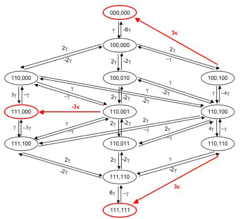
Figure 18: These are the allowed transitions between the different components of the system (272) and their rates, arising from both the decoherence (bit-flip) process (with rate $\gamma$) and the continuous error-correction process (with rate $\kappa$). Online, the transitions due to decoherence are black, and the transitions due to error correction are red.

We can use the symmetries of the process to recover the 64 coefficients of the full state. Each of the 13 coefficients represents a set of coefficients having the same number of $1$s on the left and the same number of $1$s on the right, as well as the same number of places which have $1$ on both sides. All such coefficients are equal at all times. For example, the coefficient $C_{110,011}$ is equal to all coefficients with two $1$s on the left, two $1$s on the right and exactly one place with $1$ on both sides; there are exactly six such coefficients:

$$C_{110,011}=C_{110,101}=C_{101,011}=C_{101,110}=C_{011,110}=C_{011,101}.$$

In determining the transfer rate from one coefficient to another in Fig. 2, one has to take into account the number of different coefficients of the first type which can make a transition to a coefficient of the second type of order $dt$ according to Eq. (249). The sign of the flow is determined from the phases in front of the coefficients in Eq. (271).

The eigenvalues of the matrix in Eq. (272) up to the first two lowest orders in $1/\kappa$ are presented in Table I.

Table 1: Eigenvalues of the matrix

Eigenvalues
$\lambda_{0}=0$
$\lambda_{1,2}=-\kappa$
$\lambda_{3,4}=-\kappa\pm i2\gamma$
$\lambda_{5,6}=-\kappa\pm i4\gamma$
$\lambda_{7,8}=-\kappa\pm i(\sqrt{13}+3)\gamma+\textit{O}(1/\kappa)$
$\lambda_{9,10}=-\kappa\pm i(\sqrt{13}-3)\gamma+\textit{O}(1/\kappa)$
$\lambda_{11,12}=\pm i(24/R^{2})\gamma-(144/R^{3})\gamma+\textit{O}(1/\kappa^{4})$

Obviously all eigenvalues except the first one and the last two describe fast decays with rates $\sim\kappa$. They correspond to terms in the solution which will vanish quickly after the beginning of the evolution. The eigenvalue $0$ corresponds to the asymptotic ($t\rightarrow\infty$) solution, since all other terms will eventually decay. The last two eigenvalues are those that play the main role in the evolution on a time scale $t\gg\frac{1}{\kappa}$. We see that on such a time scale, the solution will contain an oscillation with an angular frequency approximately equal to $(24/R^{2})\gamma$ which is damped by a decay factor with a rate of approximately $(144/R^{3})\gamma$. In Fig. 3 we have plotted the codeword fidelity $C_{000,000}(t)$ as a function of the dimensionless parameter $\gamma t$ for $R=100$. The graph indeed represents this type of behavior, except for very short times after the beginning ($\gamma t\sim 0.1$), where one can see a fast but small in magnitude decay (Fig. 4). The maximum magnitude of this quickly decaying term obviously decreases with $R$, since in the limit of $R\rightarrow\infty$ the fidelity should remain constantly equal to $1$.

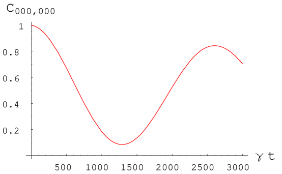
Figure 19: Long-time behavior of the three-qubit system with bit-flip noise and continuous error correction. The ratio of correction rate to decoherence rate is $R=\kappa/\gamma=100$.

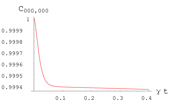
Figure 20: Short-time behavior of the three-qubit system with bit-flip noise and continuous error correction. The ratio of correction rate to decoherence rate is $R=\kappa/\gamma=100$.

From the form of the eigenvalues one can see that as $R$ increases, the frequency of the main oscillation decreases as $1/R^{2}$ while the rate of decay decreases faster, as $1/R^{3}$. Thus in the limit $R\rightarrow\infty$, the evolution approaches an oscillation with an angular frequency $(24/R^{2})\gamma$. (We formulate this statement more rigorously below.) This is the same type of evolution as that of a single qubit interacting with its environment, but the coupling constant is effectively reduced by a factor of $R^{2}/12$.

While the coupling constant serves to characterize the decoherence process in this particular case, this is not valid in general. To handle the more general situation, we propose to use the instantaneous rate of decrease of the codeword fidelity $F_{cw}$ as a measure of the effect of decoherence:

$$\Lambda(F_{cw}(t))=-\frac{dF_{cw}(t)}{dt}.$$ (273)

(In the present case, $F_{cw}=C_{000,000}$.) This quantity does not coincide with the decoherence rate in the Markovian case (which can be defined naturally from the Lindblad equation), but it is a good estimate of the rate of loss of fidelity and can be used for any decoherence model. From now on we will refer to it simply as an error rate, but we note that there are other possible definitions of instantaneous error rate suitable for non-Markovian decoherence, which in general may depend on the kind of errors they describe. Since the goal of error correction is to preserve the codeword fidelity, the quantity (273) is a useful indicator for the performance of a given scheme. Note that $\Lambda(F_{cw})$ is a function of the codeword fidelity and therefore it makes sense to use it for a comparison between different cases only for identical values of $F_{cw}$. For our example, the fact that the coupling constant is effectively reduced approximately $R^{2}/12$ times implies that the error rate for a given value of $F_{cw}$ is also reduced $R^{2}/12$ times. Similarly, the reduction of $\lambda$ by the factor $r/6$ in the Markovian case implies a reduction of $\Lambda$ by the same factor. We see that the effective reduction of the error rate increases quadratically with $\kappa^{2}$ in the non-Markovian case, whereas it increases only linearly with $\kappa$ in the Markovian case.

Now let us rigorously derive the approximate solution to this model of non-Markovian decoherence with continuous error correction. Assuming that $\gamma\ll\kappa$ (or equivalently, $R\gg 1$), the superoperator driving the evolution of the system during a time step $\delta t$ can be written as

$$e^{\mathcal{L}\delta t} = e^{\mathcal{L}_{\kappa}\delta t}+\overset{\delta t}{\underset{0}{\int}}dt^{\prime}e^{\mathcal{L}_{\kappa}(\delta t-t^{\prime})}\mathcal{L}_{\gamma}e^{\mathcal{L}_{\kappa}t^{\prime}}+\overset{\delta t}{\underset{0}{\int}}dt^{\prime}\overset{\delta t}{\underset{t^{\prime}}{\int}}dt^{\prime\prime}e^{\mathcal{L}_{\kappa}(\delta t-t^{\prime\prime})}\mathcal{L}_{\gamma}e^{\mathcal{L}_{\kappa}(t^{\prime\prime}-t^{\prime})}\mathcal{L}_{\gamma}e^{\mathcal{L}_{\kappa}t^{\prime}}+$$ (274)

$$+ \overset{\delta t}{\underset{0}{\int}}dt^{\prime}\overset{\delta t}{\underset{t^{\prime}}{\int}}dt^{\prime\prime}\overset{\delta t}{\underset{t^{\prime\prime}}{\int}}dt^{\prime\prime\prime}e^{\mathcal{L}_{\kappa}(\delta t-t^{\prime\prime\prime})}\mathcal{L}_{\gamma}e^{\mathcal{L}_{\kappa}(t^{\prime\prime\prime}-t^{\prime\prime})}\mathcal{L}_{\gamma}e^{\mathcal{L}_{\kappa}(t^{\prime\prime}-t^{\prime})}\mathcal{L}_{\gamma}e^{\mathcal{L}_{\kappa}t^{\prime}}+...$$

We have denoted the Liouvillian by $\mathcal{L}=\mathcal{L}_{\gamma}+\mathcal{L}_{\kappa}$, where $\mathcal{L}_{\kappa}\rho=\kappa\Gamma(\rho)$, and $\mathcal{L}_{\gamma}\rho=-i[H,\rho]$.

Let $\gamma\delta t\ll 1\ll\kappa\delta t$. We will derive an approximate differential equation for the evolution of $\rho(t)$ by looking at the terms of order $\delta t$ in the change of $\rho$ according to Eq. (274). When $\kappa=0$, we have $d\rho/dt=\mathcal{L}_{\gamma}\rho$, so the effect of $\mathcal{L}_{\gamma}$ on the state of the system can be seen from Eq. (272) with $\kappa$ taken equal to $0$. By the action of $\exp({\mathcal{L}_{\kappa}t})$, the different terms of the density matrix transform as follows: $\varrho_{000,000},\varrho_{111,000},\varrho_{111,111}$ remain unchanged, $\varrho_{100,100}\rightarrow e^{-\kappa t}\varrho_{100,100}+(1-e^{-\kappa t})\varrho_{000,000}$, $\varrho_{110,110}\rightarrow e^{-\kappa t}\varrho_{110,110}+(1-e^{-\kappa t})\varrho_{111,111}$, $\varrho_{110,001}\rightarrow e^{-\kappa t}\varrho_{110,001}-(1-e^{-\kappa t})\varrho_{111,000}$, and all other terms are changed as $\varrho\rightarrow e^{-\kappa t}\varrho$. Since $\kappa\delta t\gg 1$, we will ignore terms of order $e^{-\kappa\delta t}$. But from Eq. (274) it can be seen that all terms except $\varrho_{000,000},\varrho_{111,000},\varrho_{000,111},\varrho_{111,111}$ will get multiplied by the factor $e^{-\kappa\delta t}$ by the action of $\exp({\mathcal{L}_{\kappa}\delta t})$ in Eq. (274). The integrals in Eq. (274) also yield negligible factors, since every integral either gives rise to a factor of order $\delta t$ when the integration variable is trivially integrated, or a factor of $1/\kappa$ when the variable participates nontrivially in the exponent. Therefore, in the above approximation these terms of the density matrix can be neglected, which amounts to an effective evolution entirely within the code space. According to Eq. (272), the terms $\varrho_{000,000},\varrho_{111,000},\varrho_{111,111}$ can couple to each other only by a triple or higher application of $\mathcal{L}_{\gamma}$. This means that if we consider the expansion up to the lowest nontrivial order in $\gamma$, we only need to look at the triple integral in Eq. (274).

Let us consider the effect of $\exp({\mathcal{L}\delta t})$ on $C_{000,000}$. Any change can come directly only from $\varrho_{111,000}$ and $\varrho_{000,111}$. The first exponent $e^{\mathcal{L}_{\kappa}t^{\prime}}$ acts on these terms as the identity. Under the action of the first operator $\mathcal{L}_{\gamma}$ each of these two terms can transform to six terms that can eventually be transformed to $\varrho_{000,000}$. They are $\varrho_{110,000}$, $\varrho_{101,000}$, $\varrho_{011,000}$, $\varrho_{111,100}$, $\varrho_{111,010}$, $\varrho_{111,001}$, and $\varrho_{000,110}$, $\varrho_{000,101}$, $\varrho_{000,011}$, $\varrho_{100,111}$, $\varrho_{010,111}$, $\varrho_{001,111}$, with appropriate factors. The action of the second exponent is to multiply each of these new terms by $e^{-\kappa(t^{\prime\prime}-t^{\prime})}$. After the action of the second $\mathcal{L}_{\gamma}$, the action of the third exponent on the relevant resultant terms will be again to multiply them by a factor $e^{-\kappa(t^{\prime\prime\prime}-t^{\prime\prime})}$. Thus the second and the third exponents yield a net factor of $e^{-\kappa(t^{\prime\prime\prime}-t^{\prime})}$. After the second and the third $\mathcal{L}_{\gamma}$, the relevant terms that we get are $\varrho_{000,000}$ and $\varrho_{100,100}$, $\varrho_{010,010}$, $\varrho_{001,001}$, each with a corresponding factor. Finally, the last exponent acts as the identity on $\varrho_{000,000}$ and transforms each of the terms $\varrho_{100,100}$, $\varrho_{010,010}$, $\varrho_{001,001}$ into $(1-e^{-\kappa(\delta t-t^{\prime\prime\prime})})\varrho_{000,000}$. Counting the number of different terms that arise at each step, and taking into account the factors that accompany them, we obtain:

$$C_{000,000} \rightarrow C_{000,000}+\overset{\delta t}{\underset{0}{\int}}dt^{\prime}\overset{\delta t}{\underset{t^{\prime}}{\int}}dt^{\prime\prime}\overset{\delta t}{\underset{t^{\prime\prime}}{\int}}dt^{\prime\prime\prime}(24e^{-\kappa(t^{\prime\prime\prime}-t^{\prime})}-36e^{-\kappa(\delta t-t^{\prime})})C_{111,000}+\cdots$$ (275)

$$\approx C_{000,000}+C_{111,000}\frac{24}{R^{2}}\gamma\delta t+\textit{O}(\delta t^{2}).$$

Using that $C_{000,000}+C_{111,111}\approx 1$, in a similar way one obtains

$$C_{111,000}\rightarrow C_{111,000}-(2C_{000,000}-1)\frac{12}{R^{2}}\gamma\delta t+\textit{O}(\delta t^{2}).$$ (276)

For times much larger than $\delta t$, we can write the approximate differential equations

$$\frac{dC_{000,000}}{dt}=\frac{24}{R^{2}}\gamma C_{111,000},$$

$$\frac{dC_{111,000}}{dt}=-\frac{12}{R^{2}}\gamma(2C_{000,000}-1).$$ (277)

Comparing with Eq. (257), we see that the encoded qubit undergoes approximately the same type of evolution as that of a single qubit without error correction, but the coupling constant is effectively decreased $R^{2}/12$ times. The solution of Eq. (277) yields for the codeword fidelity

$$C_{000,000}(t)=\frac{1+\cos(\frac{24}{R^{2}}\gamma t)}{2}.$$ (278)

This solution is valid only with precision $\textit{O}(1/R)$ for times $\gamma t\ll R^{3}$. This is because we ignored terms whose magnitudes are always of order $\textit{O}(1/R)$ and ignored changes of order $\textit{O}(\gamma\delta t/R^{3})$ per time step $\delta t$ in the other terms. The latter changes could accumulate with time and become of the order of unity for times $\gamma t\approx R^{3}$, which is why the approximate solution is invalid for such times. In fact, if one carries out the expansion (274) to fourth order in $\gamma$, one obtains the approximate equations

$$\frac{dC_{000,000}}{dt}=\frac{24}{R^{2}}\gamma C_{111,000}-\frac{72}{R^{3}}\gamma(2C_{000,000}-1),$$

$$\frac{dC_{111,000}}{dt}=-\frac{12}{R^{2}}\gamma(2C_{000,000}-1)-\frac{144}{R^{3}}\gamma C_{111,000},$$ (279)

which yield for the fidelity

$$C_{000,000}(t)=\frac{1+e^{-144\gamma t/R^{3}}\cos(24\gamma t/R^{2})}{2}.$$ (280)

We see that in addition to the effective error process which is of the same type as that of a single qubit, there is an extra Markovian bit-flip process with rate $72\gamma/R^{3}$. This Markovian behavior is due to the Markovian character of our error-correcting procedure which, at this level of approximation, is responsible for the direct transfer of weight between $\varrho_{000,000}$ and $\varrho_{111,111}$, and between $\varrho_{111,000}$ and $\varrho_{000,111}$. The exponential factor explicitly reveals the range of applicability of the solution (278): with precision $\textit{O}(1/R)$, it is valid only for times $\gamma t$ of up to order $R^{2}$. For times of the order of $R^{3}$, the decay becomes significant and cannot be neglected. The exponential factor may also play an important role for short times of up to order $R$, where its contribution is bigger than that of the cosine. But in the latter regime the difference between the cosine and the exponent is of order $\textit{O}(1/R^{2})$, which is negligible for the precision that we consider.

In general, the effective evolution that one obtains in the limit of high error-correction rate does not have to approach a form identical to that of a single decohering qubit. The reason we obtain such behavior here is that for this particular model the lowest order of uncorrectable errors that transform the state within the code space is 3, and three-qubit errors have the form of an encoded $X$ operation. Furthermore, the symmetry of the problem ensured an identical evolution of the three qubits in the code. For general stabilizer codes, the errors that a single qubit can undergo are not limited to bit flips only. Therefore, different combinations of single-qubit errors may lead to different types of lowest-order uncorrectable errors inside the code space, none of which in principle has to represent an encoded version of the single-qubit operations that compose it. In addition, if the noise is different for the different qubits, there is no unique single-qubit error model to compare to. Nevertheless, we will show that with regard to the effective decrease in the error-correction rate, general stabilizer codes will exhibit the same qualitative performance.

5.4   Relation to the Zeno regime

The effective continuous evolution (277) was derived under the assumption that $\gamma\delta t\ll 1\ll\kappa\delta t$. The first inequality implies that $\delta t$ can be considered within the Zeno time scale of the system’s evolution without error correction. On the other hand, from the relation between $\kappa$ and $\tau_{c}$ in (242) we see that $\tau_{c}\ll\delta t$. Therefore, the time for implementing a weak error-correcting operation has to be sufficiently small so that on the Zeno time scale the error-correction procedure can be described approximately as a continuous Markovian process. This suggests a way of understanding the quadratic enhancement in the non-Markovian case based on the properties of the Zeno regime.

Let us consider again the single-qubit code from Section 5.2, but this time let the error model be any Hamiltonian-driven process. We assume that the qubit is initially in the state $|0\rangle$, i.e., the state of the system including the bath has the form $\rho(0)=|0\rangle\langle 0|\otimes\rho_{B}(0)$. For times smaller than the Zeno time $\delta t_{Z}$, the evolution of the fidelity without error correction can be described by Eq. (247). Equation (247) naturally defines the Zeno regime in terms of $\alpha$ itself:

$$\alpha\geq\alpha_{Z}\equiv 1-C\delta t_{Z}^{2}.$$ (281)

For a single time step $\Delta t\ll\delta t_{Z}$, the change in the fidelity is

$$\alpha\rightarrow\alpha-2\sqrt{C}\sqrt{1-\alpha}\Delta t+\textit{O}(\Delta t^{2}).$$ (282)

On the other hand, the effect of error correction during a time step $\Delta t$ is

$$\alpha\rightarrow\alpha+\kappa(1-\alpha)\Delta t+\textit{O}(\Delta t^{2}),$$ (283)

i.e., it tends to oppose the effect of decoherence. If both processes happen simultaneously, the effect of decoherence will still be of the form (282), but the coefficient $C$ may vary with time. This is because the presence of error-correction opposes the decrease of the fidelity and consequently can lead to an increase in the time for which the fidelity remains within the Zeno range. If this time is sufficiently long, the state of the environment could change significantly under the action of the Hamiltonian, thus giving rise to a different value for $C$ in Eq. (282) according to Eq. (248).

Note that the strength of the Hamiltonian puts a limit on $C$, and therefore this constant can vary only within a certain range. The equilibrium fidelity $\alpha_{*}^{\rm NM}$ that we obtained for the error model in Section 5.2, can be thought of as the point at which the effects of error and error correction cancel out. For a general model, where the coefficient $C$ may vary with time, this leads to a quasi-stationary equilibrium. From Eqs. (282) and (283), one obtains the equilibrium fidelity

$$\alpha_{*}^{\rm NM}\approx 1-\frac{4C}{\kappa^{2}}.$$ (284)

In agreement with what we obtained in Section 5.2, the equilibrium fidelity differs from $1$ by a quantity proportional to $1/\kappa^{2}$. This quantity is generally quasi-stationary and can vary within a limited range. If one assumes a Markovian error model, for short times the fidelity changes linearly with time which leads to $1-\alpha_{*}^{\rm M}\propto 1/\kappa$. Thus the difference can be attributed to the existence of a Zeno regime in the non-Markovian case.

But what happens in the case of non-trivial codes? As we saw, there the state decays inside the code space and therefore can be highly correlated with the environment. Can we talk about a Zeno regime then? It turns out that the answer is positive. Assuming that each qubit undergoes an independent error process, then up to first order in $\Delta t$ the Hamiltonian cannot map terms in the code space to other terms without detectable errors. (This includes both terms in the code space and terms from the hidden part, like $\varrho_{111,000}$ in the example of the bit-flip code.) It can only transform terms from the code space into traceless terms from the hidden part which correspond to single-qubit errors (like $\varrho_{100,000}$ in the same example). Let $|\bar{0}\rangle$, $|\bar{1}\rangle$ be the two logical codewords and $|\psi_{i}\rangle$ be an orthonormal basis that spans the space of all single-qubit errors. Then in the basis $|\bar{0}\rangle$, $|\bar{1}\rangle$, $|\psi_{i}\rangle$, all the terms that can be coupled directly to terms inside the code space are $|\bar{0}\rangle\langle\psi_{i}|$, $|\psi_{i}\rangle\langle\bar{0}|$, $|\bar{1}\rangle\langle\psi_{i}|$, $|\psi_{i}\rangle\langle\bar{1}|$. From the condition of positivity of the density matrix, one can show that the coefficients in front of these terms are at most $\sqrt{\alpha(1-\alpha)}$ in magnitude, where $\alpha$ is the code-space fidelity. This implies that for small enough $1-\alpha$, the change in the code-space fidelity is of the type (282), which is Zeno-like behavior. Then using only the properties of the Zeno behavior as we did above, we can conclude that the weight outside the code space will be kept at a quasi-stationary value of order $1/\kappa^{2}$. Since uncorrectable errors enter the code space through the action of the error-correction procedure, which misinterprets some multi-qubit errors in the error space, the effective error rate will be limited by a factor proportional to the weight in the error space. That is, this will lead to an effective decrease of the error rate at least by a factor proportional to $1/\kappa^{2}$.

The accumulation of uncorrectable errors in the Markovian case is similar, except that in this case there is a direct transfer of errors between the code space and the visible part of the error space. In both cases, the error rate is effectively reduced by a factor which is roughly proportional to the inverse of the weight in the error space, and therefore the difference in the performance comes from the difference in this weight. The quasi-stationary equilibrium value of the code-space fidelity establishes a quasi-stationary flow between the code space and the error space. One can think that this flow effectively takes non-erroneous weight from the code space, transports it through the error space where it accumulates uncorrectable errors, and brings it back into the code space. Thus by minimizing the weight outside the code space, error correction creates a “bottleneck” which reduces the rate at which uncorrectable errors accumulate.

Finally, a brief remark about the resources needed for quadratic reduction of the error rate. As pointed out above, two conditions are involved: one concerns the rate of error correction; the other concerns the time resolution of the weak error-correcting operations. Both of these quantities must be sufficiently large. There is, however, an interplay between the two, which involves the strength of the interaction required to implement the weak error-correcting map (241). Let us imagine that the weak map is implemented by making the system interact weakly with an ancilla in a given state, after which the ancilla is discarded. The error-correction procedure consists of a sequence of such interactions, and can be thought of as a cooling process which takes away the entropy accumulated in the system as a result of correctable errors. If the time for which a single ancilla interacts with the system is $\tau_{c}$, one can verify that the parameter $\epsilon$ in Eq. (241) would be proportional to $g^{2}\tau_{c}^{2}$, where $g$ is the coupling strength between the system and the ancilla. From Eq. (242) we then obtain that

$$\kappa\propto g^{2}\tau_{c}.$$ (285)

The two parameters that can be controlled are the interaction time and the interaction strength, and they determine the error-correction rate. Thus if $g$ is kept constant, a decrease in the interaction time $\tau_{c}$ leads to a proportional decrease in $\kappa$, which may be undesirable. In order to achieve a good working regime, one may need to adjust both $\tau_{c}$ and $g$. But it has to be pointed out that in some situations decreasing $\tau_{c}$ alone can prove advantageous, if it leads to a time resolution revealing the non-Markovian character of an error model which was previously described as Markovian. The quadratic enhancement of the performance as a function of $\kappa$ may compensate the decrease in $\kappa$, thus leading to a seemingly paradoxical result: better performance with a lower error-correction rate.

5.5   Summary and outlook

In this chapter we studied the performance of a particular continuous quantum error-correction scheme for non-Markovian errors. We analyzed the evolution of the single-qubit code and the three-qubit bit-flip code in the presence of continuous error correction for a simple non-Markovian bit-flip error model. This enabled us to understand the workings of the error-correction scheme, and the mechanism whereby uncorrectable errors accumulate. The fidelity of the state with the code space in both examples quickly reaches an equilibrium value, which can be made arbitrarily close to $1$ by a sufficiently high rate of error correction. The weight of the density matrix outside the code space scales as $1/\kappa$ in the Markovian case, while it scales as $1/\kappa^{2}$ in the non-Markovian case. Correspondingly, the rate at which uncorrectable errors accumulate in the three-qubit code is proportional to $1/\kappa$ in the Markovian case, and to $1/\kappa^{2}$ in the non-Markovian case. These differences have the same cause, since the equilibrium weight in the error space is closely related to the rate of uncorrectable error accumulation.

The quadratic difference in the error weight between the Markovian and non-Markovian cases can be attributed to the existence of a Zeno regime in the non-Markovian case. Regardless of the correlations between the density matrix inside the code space and the environment, if the lowest-order errors are correctable by the code, there exists a Zeno regime in the evolution of the code-space fidelity. The effective reduction of the error rate with the rate of error correction for non-Markovian error models depends crucially on the assumption that the time resolution of the continuous error correction is much shorter than the Zeno time scale of the evolution without error correction. This suggests that decreasing the time for a single (infinitesimal) error-correcting operation can lead to an increase in the performance of the scheme, even if the average error-correction rate goes down.

While here we have only considered codes for the correction of single-qubit errors, our results can be extended to other types of codes and errors as well. As long as the error process only produces errors correctable by the code to lowest order, an argument analogous to the one given here shows that a Zeno regime will exist, which leads to an enhancement in the error-correction performance. Unfortunately, it is very difficult to describe the evolution of a system with a continuous correction protocol, based on a general error-correction code and subject to general non-Markovian interactions with the environment. This is especially true if one must include the evolution of a complicated environment in the description, as would be necessary in general. A more practical step in this direction might be to find an effective description for the evolution of the reduced density matrix of the system subject to decoherence plus error correction, using projection techniques like the Nakajima-Zwanzig or the TCL master equations. Since one is usually interested in the evolution during initial times before the codeword fidelity decreases significantly, a perturbation approach could be useful. This is a subject for further research.

5.6   Appendix: Implementation of the quantum-jump error-correcting process via weak measurements and weak unitary operations

Here we show how the weak CPTP map (241) for the bit-flip code can be implemented using weak measurements and weak unitary operations. We also present a similar scheme for codes that correct arbitrary-single qubit errors, which yields a weak map different from (241) but one that also results in the strong error-correcting map $\Phi(\rho)$ when exponentiated. To introduce our construction, we start again with the single-qubit code with stabilizer $\langle Z\rangle$.

5.6.1   The single-qubit model

Consider the completely positive map corresponding to the strong error-correcting operation for the single-qubit code:

$$\Phi(\rho)=X|1\rangle\langle 1|\rho|1\rangle\langle 1|X+|0\rangle\langle 0|\rho|0\rangle\langle 0|=|0\rangle\langle 1|\rho|1\rangle\langle 0|+|0\rangle\langle 0|\rho|0\rangle\langle 0|.$$ (286)

Observe that this transformation can also be written as

$$\Phi(\rho)=|0\rangle\langle+|\rho|+\rangle\langle 0|+|0\rangle\langle-|\rho|-\rangle\langle 0|=ZR|+\rangle\langle+|\rho|+\rangle\langle+|RZ+XR|-\rangle\langle-|\rho|-\rangle\langle-|RX,$$ (287)

where $|\pm\rangle=(|0\rangle\pm|1\rangle)/\sqrt{2}$ and

$$R=\frac{1}{\sqrt{2}}\begin{pmatrix}1&1\\ 1&-1\\ \end{pmatrix}$$ (288)

is the Hadamard gate. Therefore the same error-correcting operation can be implemented as a measurement in the $|\pm\rangle$ basis (measurement of the operator $X$), followed by a unitary conditioned on the outcome: if the outcome is ’+’, we apply $ZR$; if the outcome is ’-’, we apply $XR$. This choice of unitaries is not unique—for example, we could apply just $R$ instead of $ZR$ after outcome ’+’. But this particular choice has a convenient geometric interpretation—the unitary $ZR$ corresponds to a rotation around the Y-axis by an angle $\pi/2$: $ZR=e^{i\frac{\pi}{2}\frac{Y}{2}}$, and $XR$ corresponds to a rotation around the same axis by an angle $-\pi/2$: $ZR=e^{-i\frac{\pi}{2}\frac{Y}{2}}$.

A weak version of the above error-correcting operation can be constructed by taking the corresponding weak measurement of the operator $X$, followed by a weak rotation around the Y-axis, whose direction is conditioned on the outcome:

$$\begin{split}\rho\rightarrow\frac{I+i\epsilon^{\prime}Y}{\sqrt{1+{\epsilon^{\prime}}^{2}}}\sqrt{\frac{I+\epsilon X}{2}}\rho\sqrt{\frac{I+\epsilon X}{2}}\frac{I-i\epsilon^{\prime}Y}{\sqrt{1+{\epsilon^{\prime}}^{2}}}+\\ +\frac{I-i\epsilon^{\prime}Y}{\sqrt{1+{\epsilon^{\prime}}^{2}}}\sqrt{\frac{I-\epsilon X}{2}}\rho\sqrt{\frac{I-\epsilon X}{2}}\frac{I+i\epsilon^{\prime}Y}{\sqrt{1+{\epsilon^{\prime}}^{2}}}.\end{split}$$ (289)

Here $\epsilon$ and $\epsilon^{\prime}$ are small parameters. From the symmetry of this map it can be seen that if the map is applied to a state which lies on the Z-axis, the resultant state will still lie on the Z-axis. Whether the state will move towards $|0\rangle\langle 0|$ or towards $|1\rangle\langle 1|$, depends on the relation between $\epsilon$ and $\epsilon^{\prime}$. Since our goal is to protect the state from drifting away from $|0\rangle\langle 0|$ due to bit-flip decoherence, we will assume that the state lies on the Z-axis in the northern hemisphere (although the transformation we will obtain works for any kind of decoherence where the state need nor remain on the Z-axis). We would like, if possible, to choose the relation between the parameters $\epsilon$ and $\epsilon^{\prime}$ in such a way that the effect of this map on any state on the Z-axis to be to move the state towards $|0\rangle\langle 0|$.

In order to calculate the effect of this map on a given state, it is convenient to write the state in the $|\pm\rangle$ basis. For a state on the Z-axis, $\rho=\alpha|0\rangle\langle 0|+(1-\alpha)|1\rangle\langle 1|$, we have

$$\rho=\frac{1}{2}|+\rangle\langle+|+\frac{1}{2}|-\rangle\langle-|+(2\alpha-1)\left(\frac{1}{2}|+\rangle\langle-|+\frac{1}{2}|-\rangle\langle+|\right).$$ (290)

For the action of our map on the state (290) we obtain:

$$\rho\rightarrow\frac{1}{2}|+\rangle\langle+|+\frac{1}{2}|-\rangle\langle-|+\frac{(1-{\epsilon^{\prime}}^{2})\sqrt{1-\epsilon^{2}}(2\alpha-1)+2\epsilon\epsilon^{\prime}}{1+{\epsilon^{\prime}}^{2}}\left(\frac{1}{2}|+\rangle\langle-|+\frac{1}{2}|-\rangle\langle+|\right).$$ (291)

Thus we can think that upon this transformation the parameter $\alpha$ transforms to $\alpha^{\prime}$, where

$$2\alpha^{\prime}-1=\frac{(1-{\epsilon^{\prime}}^{2})\sqrt{1-\epsilon^{2}}(2\alpha-1)+2\epsilon\epsilon^{\prime}}{1+{\epsilon^{\prime}}^{2}}.$$ (292)

If it is possible to choose the relation between $\epsilon$ and $\epsilon^{\prime}$ in such a way that $\alpha^{\prime}\geq\alpha$ for every $0\leq\alpha\leq 1$, then clearly the state must remain invariant when $\alpha=1$. Imposing this requirement, we obtain

$$\epsilon=\frac{2\epsilon^{\prime}}{1+{\epsilon^{\prime}}^{2}},$$ (293)

or equivalently

$$\epsilon^{\prime}=\frac{1-\sqrt{1-\epsilon^{2}}}{\epsilon}.$$ (294)

Substituting back in (292), we can express

$$\alpha^{\prime}-\alpha=\frac{4{\epsilon^{\prime}}^{2}}{(1+{\epsilon^{\prime}}^{2})^{2}}(1-\alpha)\geq 0.$$ (295)

We see that the coefficient $\alpha$ (which is the fidelity of our state with $|0\rangle\langle 0|$) indeed increases after every application of our weak completely positive map (Fig.1). The amount by which it increases for fixed $\epsilon^{\prime}$ depends on $\alpha$ and becomes smaller as $\alpha$ approaches 1.

Since we will be taking the limit $\epsilon\rightarrow 0$, we can write Eq. (294) as

$$\epsilon^{\prime}=\frac{\epsilon}{2}+\textit{O}(\epsilon^{3}).$$ (296)

If we define the relation between the time step $\tau_{c}$ and $\epsilon$ as in Eq. (242), for the effect of the CPTP map (289) on an arbitrary state of the form $\rho=\alpha|0\rangle\langle 0|+\beta|0\rangle\langle 1|+\beta^{*}|1\rangle\langle 0|+(1-\alpha)|1\rangle\langle 1|$, $\alpha\in R$, $\beta\in C$, we obtain

$$\alpha\rightarrow\alpha+(1-\alpha)\kappa\tau_{c},$$ (297)

$$\beta\rightarrow\sqrt{1-\kappa\tau_{c}}\beta=\beta-\frac{1}{2}\kappa\beta\tau_{c}+O({\tau_{c}}^{2}).$$ (298)

This is exactly the map (241) for $\Phi(\rho)$ given by Eq. (286).

5.6.2   The bit-flip code

While in the toy model from the previous section we had to protect a given state from errors, here we have to protect the whole subspace spanned by $|\overline{0}\rangle$ and $|\overline{1}\rangle$. This makes a geometric visualization of the problem significantly more difficult than in the previous case, which is why we will take a different approach.

In the single-qubit model we saw how to protect a qubit in state $|0\rangle$ from bit-flip errors. Similarly we could protect a qubit in state $|1\rangle$; the only difference is that the weak unitaries following the two outcomes of the weak measurement of $X$ have to be exchanged. For the three-qubit bit-flip code, every block of the code lies in the subspace spanned by the codewords $|000\rangle$ and $|111\rangle$, i.e., each qubit is in state $|0\rangle$ when the other two qubits are in state $|00\rangle$, or in state $|1\rangle$ when the other qubits are in state $|11\rangle$. This correlation is what makes it possible for the code to correct single-qubit bit-flip errors without ever acquiring information about the actual state of the system. We propose to utilize this correlation in a three-qubit scheme which protects each qubit by applying to it the corresponding single-qubit scheme for either $|0\rangle$ or $|1\rangle$ depending on the value of the other two qubits. This, of course, has to be done without acquiring information about the encoded state.

Just as in the single-qubit case, the scheme consist of weak measurements followed by weak unitaries conditioned on the outcomes of the measurements. For error correction on the first qubit, we propose the weak measurement with measurement operators

$$M^{1}_{\pm}=\sqrt{\frac{I{\pm}\epsilon X}{2}}\otimes(|00\rangle\langle 00|+|11\rangle\langle 11|)+\frac{I}{\sqrt{2}}\otimes(|01\rangle\langle 01|+|10\rangle\langle 10|),$$ (299)

where $\sqrt{\frac{I{\pm}\epsilon X}{2}}$ are the same weak measurement operators that we used in (289), acting on the first qubit. This measurement can be thought of as a weak measurement of the operator $X\otimes(|00\rangle\langle 00|+|11\rangle\langle 11|)$. In order to understand its effect better, consider the expansion of the density matrix of our system in the computational basis of the three qubits in a given block of the code. Assuming that the state begins inside the code space and that the system decoheres through single-qubit bit-flip channels, the density matrix at any time can be written as a linear combination of the following terms: $|000\rangle\langle 000|$,$|000\rangle\langle 111|$, $|111\rangle\langle 000|$, $|111\rangle\langle 111|$, $|100\rangle\langle 100|$, $|100\rangle\langle 011|$, $|011\rangle\langle 100|$, $|011\rangle\langle 011|$, $|010\rangle\langle 010|$, $|010\rangle\langle 101|$, $|101\rangle\langle 010|$, $|101\rangle\langle 101|$, $|001\rangle\langle 001|$, $|001\rangle\langle 110|$,
$|110\rangle\langle 001|$, $|110\rangle\langle 110|$. For those terms in the expansion for which the second and third qubits are in the subspace spanned by $|00\rangle$ and $|11\rangle$, the effect of this measurement will be the same as the effect of a weak single-qubit measurement of $X$ on the first qubit. Those terms in which the second and third qubits are in the subspace spanned by $|01\rangle$ and $|10\rangle$ will not be affected by the measurement. This is because the three-qubit bit-flip code cannot distinguish multi-qubit errors from single-qubit errors; the subspaces corresponding to two- and three-qubit errors are the same as the subspaces corresponding to single-qubit or no errors. This is why, if the second and third qubits have different values, the error-correction scheme will assume that an error has occurred on one of these two qubits and will not apply any correction on the first qubit.

The unitary operation conditioned on the outcome of the measurement is

$$U^{1}_{\pm}=\frac{I\pm i\epsilon^{\prime}Y}{\sqrt{1+{\epsilon^{\prime}}^{2}}}\otimes|00\rangle\langle 00|+\frac{I\mp i\epsilon^{\prime}Y}{\sqrt{1+{\epsilon^{\prime}}^{2}}}\otimes|11\rangle\langle 11|+I\otimes(|01\rangle\langle 01|+|10\rangle\langle 10|).$$ (300)

This is a weak unitary driven by the Hamiltonian $\pm Y\otimes(|00\rangle\langle 00|-|11\rangle\langle 11|)$. Again, it is designed in such a way that those components of the density matrix which correspond to an error on the second or third qubits will undergo no transformation, while the terms for which the second and third qubits have the same value (these are the same terms that have undergone non-trivial transformation during the measurement) will undergo a rotation of the first qubit analogous to that from the single-qubit model. One can verify that the only terms that undergo non-trivial transformation after the completely positive map $\rho\rightarrow U^{1}_{+}M^{1}_{+}\rho M^{1}_{+}{U^{1}_{+}}^{\dagger}+U^{1}_{-}M^{1}_{-}\rho M^{1}_{-}{U^{1}_{-}}^{\dagger}$ are:

$$\begin{split}|100\rangle\langle 100|\rightarrow(1-\kappa\tau_{c})|100\rangle\langle 100|+\kappa\tau_{c}|000\rangle\langle 000|,\\ |100\rangle\langle 011|\rightarrow(1-\kappa\tau_{c})|100\rangle\langle 011|+\kappa\tau_{c}|000\rangle\langle 111|,\\ |011\rangle\langle 100|\rightarrow(1-\kappa\tau_{c})|011\rangle\langle 100|+\kappa\tau_{c}|111\rangle\langle 000|,\\ |011\rangle\langle 011|\rightarrow(1-\kappa\tau_{c})|011\rangle\langle 011|+\kappa\tau_{c}|111\rangle\langle 111|.\\ |100\rangle\langle\overline{\phi}|\rightarrow(1-\frac{1}{2}\kappa\tau_{c})|100\rangle\langle\overline{\phi}|,\hskip 5.69046pt|\overline{\phi}\rangle\langle 100|\rightarrow(1-\frac{1}{2}\kappa\tau_{c})|\overline{\phi}\rangle\langle 100|\\ |011\rangle\langle\overline{\phi}|\rightarrow(1-\frac{1}{2}\kappa\tau_{c})|011\rangle\langle\overline{\phi}|,\hskip 5.69046pt|\overline{\phi}\rangle\langle 011|\rightarrow(1-\frac{1}{2}\kappa\tau_{c})|\overline{\phi}\rangle\langle 011|\end{split}$$ (301)

where $|\overline{\phi}\rangle$ is any state orthogonal to the subspace spanned by $|100\rangle$ and $|011\rangle$. We see that the effect of this operation on the terms that correspond to bit flip on the first qubit is to correct these terms by the same amount as in the single-qubit error-correction scheme. All other terms remain unchanged. If we write the state of the system at a given moment as

$$\rho=a\rho(0)+b_{1}X_{1}\rho(0)X_{1}+b_{2}X_{2}\rho(0)X_{2}+b_{3}X_{3}\rho(0)X_{3}+$$ (302)

$$+c_{1}X_{2}X_{3}\rho(0)X_{2}X_{3}+c_{2}X_{1}X_{3}\rho(0)X_{1}X_{3}+c_{3}X_{1}X_{2}\rho(0)X_{1}X_{2}+dX_{1}X_{2}X_{3}\rho(0)X_{1}X_{2}X_{3},$$

where $\rho(0)$ is the initial state, then the effect of the above completely positive map is:

$$\begin{split}a\rightarrow a+b_{1}4\kappa\tau_{c},\hskip 5.69046ptb_{1}\rightarrow b_{1}-b_{1}4\kappa\tau_{c},\hskip 5.69046ptb_{2}\rightarrow b_{2},\hskip 5.69046ptb_{3}\rightarrow b_{3},\\ c_{1}\rightarrow c_{1}-c_{1}4\kappa\tau_{c},\hskip 5.69046ptc_{2}\rightarrow c_{2},\hskip 5.69046ptc_{3}\rightarrow c_{3},\hskip 5.69046ptd\rightarrow d+c_{1}4\kappa\tau_{c}.\end{split}$$ (303)

We apply the same correction ($\rho\rightarrow U^{i}_{+}M^{i}_{+}\rho M^{i}_{+}{U^{i}_{+}}^{\dagger}+U^{i}_{-}M^{i}_{-}\rho M^{i}_{-}{U^{i}_{-}}^{\dagger}$) to each of the other two qubits ($i=2,3$) as well. One can easily see that the effect of all three corrections (up to first order in $\Delta t$) is equivalent to the map (241) with $\Phi(\rho)$ given in Eq. (240).

5.6.3   General single-error-correcting stabilizer codes

We now proceed to generalizing this scheme to error-correcting codes that correct arbitrary single-qubit errors. A stabilizer code which is able to correct arbitrary single-qubit errors, has the property that a single-qubit $X$, $Y$ or $Z$ error on a state inside the code space, sends that state to a subspace orthogonal to the code space [67]. One can verify that this implies that any two orthogonal codewords can be written as

$$|\overline{0}\rangle=\frac{1}{\sqrt{2}}|0\rangle|\psi^{0}_{0}\rangle+\frac{1}{\sqrt{2}}|1\rangle|\psi^{0}_{1}\rangle,$$

$$|\overline{1}\rangle=\frac{1}{\sqrt{2}}|0\rangle|\psi^{1}_{0}\rangle+\frac{1}{\sqrt{2}}|1\rangle|\psi^{1}_{1}\rangle,$$ (304)

where $|\psi^{i}_{j}\rangle$, $i,j=0,1$ form an orthonormal set. Here we have expanded the codewords in the computational basis (the eigenbasis of $Z$) of the first qubit, but the same can be done with respect to any qubit in the code. Note that an $X$, $Y$, or $Z$ error on one of the other qubits sends each of the vectors $|\psi^{i}_{j}\rangle$ to a subspace orthogonal to the subspace spanned by $|\psi^{i}_{j}\rangle$, $i,j=0,1$. This can be shown to follow from the fact that different single-qubit errors send the code space to different orthogonal subspaces. An exception is the case of degenerate codes where the error in question has the same effect on a codeword as an error on the first qubit. In such a case, however, we can assume that the error has occurred on the first qubit. The weak operation for correcting bit flips on a given qubit (say the first one) is therefore constructed similarly to that for the bit-flip code. We first apply the weak measurement

$$M^{1}_{\pm}=\sqrt{\frac{I{\pm}\epsilon X}{2}}\otimes(|\psi^{0}_{0}\rangle\langle\psi^{0}_{0}|+|\psi^{0}_{1}\rangle\langle\psi^{0}_{1}|+|\psi^{1}_{0}\rangle\langle\psi^{1}_{0}|+|\psi^{1}_{1}\rangle\langle\psi^{1}_{1}|)+$$

$$+\frac{I}{\sqrt{2}}\otimes(I^{n-1}-|\psi^{0}_{0}\rangle\langle\psi^{0}_{0}|-|\psi^{0}_{1}\rangle\langle\psi^{0}_{1}|-|\psi^{1}_{0}\rangle\langle\psi^{1}_{0}|-|\psi^{1}_{1}\rangle\langle\psi^{1}_{1}|),$$ (305)

where $I^{n-1}$ is the identity on the space of all qubits in the code except the first one. This can be thought of as a weak measurement of the operator $X(|\psi^{0}_{0}\rangle\langle\psi^{0}_{0}|+|\psi^{0}_{1}\rangle\langle\psi^{0}_{1}|+|\psi^{1}_{0}\rangle\langle\psi^{1}_{0}|+|\psi^{1}_{1}\rangle\langle\psi^{1}_{1}|)$. The measurement is followed by the unitary

$$U^{1}_{\pm}=\frac{I\pm i\epsilon^{\prime}Y}{\sqrt{1+{\epsilon^{\prime}}^{2}}}\otimes(|\psi^{0}_{0}\rangle\langle\psi^{0}_{0}|+|\psi^{1}_{0}\rangle\langle\psi^{1}_{0}|)+\frac{I\mp i\epsilon^{\prime}Y}{\sqrt{1+{\epsilon^{\prime}}^{2}}}\otimes(|\psi^{0}_{1}\rangle\langle\psi^{0}_{1}|+|\psi^{1}_{1}\rangle\langle\psi^{1}_{1}|)+$$

$$+I\otimes(I^{n-1}-|\psi^{0}_{0}\rangle\langle\psi^{0}_{0}|-|\psi^{0}_{1}\rangle\langle\psi^{0}_{1}|-|\psi^{1}_{0}\rangle\langle\psi^{1}_{0}|-|\psi^{1}_{1}\rangle\langle\psi^{1}_{1}|)$$ (306)

conditioned on the outcome. The Hamiltonian driving this unitary is $\pm Y(|\psi^{0}_{0}\rangle\langle\psi^{0}_{0}|+|\psi^{1}_{0}\rangle\langle\psi^{1}_{0}|-|\psi^{0}_{1}\rangle\langle\psi^{0}_{1}|-|\psi^{1}_{1}\rangle\langle\psi^{1}_{1}|)$. It is easy to verify that the effect of the corresponding completely positive map is analogous to that for the bit-flip code. The action of each of the operators $U^{1}_{+}M^{1}_{+}$ and $U^{1}_{-}M^{1}_{-}$ can be summarized as follows:

$$U^{1}_{\pm}M^{1}_{\pm}|i\rangle|\phi\rangle=\frac{1}{\sqrt{2}}|i\rangle|\phi\rangle,\hskip 8.5359pt\textrm{for}\hskip 5.69046pt|\phi\rangle\in I^{n-1}-\underset{j,k}{\sum}|\psi^{j}_{k}\rangle\langle\psi^{j}_{k}|,$$ (307)

$$U^{1}_{\pm}M^{1}_{\pm}|j\rangle|\psi^{i}_{k}\rangle=\sqrt{\frac{1-\kappa\tau_{c}}{2}}|j\rangle|\psi^{i}_{k}\rangle\pm\sqrt{\frac{\kappa\tau_{c}}{2}}|k\rangle|\psi^{i}_{k}\rangle,\hskip 8.5359pt\textrm{for}\hskip 5.69046ptj\neq k,$$ (308)

$$U^{1}_{\pm}M^{1}_{\pm}|j\rangle|\psi^{i}_{k}\rangle=|j\rangle|\psi^{i}_{k}\rangle,\hskip 8.5359pt\textrm{for}\hskip 5.69046ptj=k.$$ (309)

This implies that the effect of the map $\sigma\rightarrow U^{1}_{+}M^{1}_{+}\sigma M^{1}_{+}{U^{1}_{+}}^{\dagger}+U^{1}_{-}M^{1}_{-}\sigma M^{1}_{-}{U^{1}_{-}}^{\dagger}$ on a bit-flip error on the first qubit of a codeword $\rho$ is:

$$X_{1}\rho X_{1}\rightarrow(1-\kappa\tau_{c})X_{1}\rho X_{1}+\kappa\tau_{c}\rho,$$ (310)

$$X_{1}\rho\rightarrow(1-\frac{1}{2}\kappa\tau_{c})X_{1}\rho,$$ (311)

$$\rho X_{1}\rightarrow(1-\frac{1}{2}\kappa\tau_{c})\rho X_{1}.$$ (312)

Just like in the bit-flip code, the error-correcting procedure for the case where each qubit decoheres through an independent bit-flip channel consists of simultaneous corrections of all qubits ($i=1,2,...,n$) by continuous application of the maps $\sigma\rightarrow U^{i}_{+}M^{i}_{+}\sigma M^{i}_{+}{U^{i}_{+}}^{\dagger}+U^{i}_{-}M^{i}_{-}\sigma M^{i}_{-}{U^{i}_{-}}^{\dagger}$.

From (304) it can be seen that the codewords have analogous forms when expanded in the eigenbasis of another Pauli operator ($X$ or $Y$) acting on a given qubit:

$$|\overline{0}\rangle=\frac{1}{\sqrt{2}}|x_{+}\rangle|\psi^{0}_{x_{+}}\rangle+\frac{1}{\sqrt{2}}|x_{-}\rangle|\psi^{0}_{x_{-}}\rangle=\frac{1}{\sqrt{2}}|y_{+}\rangle|\psi^{0}_{y_{+}}\rangle+\frac{1}{\sqrt{2}}|y_{-}\rangle|\psi^{0}_{y_{-}}\rangle,$$

$$|\overline{1}\rangle=\frac{1}{\sqrt{2}}|x_{+}\rangle|\psi^{1}_{x_{+}}\rangle+\frac{1}{\sqrt{2}}|x_{-}\rangle|\psi^{1}_{x_{-}}\rangle=\frac{1}{\sqrt{2}}|y_{+}\rangle|\psi^{1}_{y_{+}}\rangle+\frac{1}{\sqrt{2}}|y_{-}\rangle|\psi^{1}_{y_{-}}\rangle.$$ (313)

Here

$$|x_{\pm}\rangle=(-i)^{\frac{1\mp 1}{2}}\frac{|0\rangle\pm|1\rangle}{\sqrt{2}}$$ (314)

and

$$|y_{\pm}\rangle=\frac{|0\rangle\pm i|1\rangle}{\sqrt{2}}$$ (315)

are eigenbases of $X$ and $Y$ respectively, and

$$|\psi^{i}_{x_{\pm}}\rangle=i^{\frac{1\mp 1}{2}}\frac{|\psi^{i}_{0}\rangle\pm|\psi^{i}_{1}\rangle}{\sqrt{2}},\hskip 2.84544pti=0,1$$ (316)

and

$$|\psi^{i}_{y_{\pm}}\rangle=\frac{|\psi^{i}_{0}\rangle\mp i|\psi^{i}_{1}\rangle}{\sqrt{2}},\hskip 2.84544pti=0,1$$ (317)

are orthonormal sets. The reason why we have chosen these particular overall phases in the definition of the eigenvectors of $X$ and $Y$, is that we want to have our expressions explicitly symmetric with respect to cyclic permutations of $X$, $Y$ and $Z$. More precisely, the expansions of the operators $X$, $Y$, $Z$ in the $|0,1\rangle$ basis are the same as the expansions of $Y$, $Z$, $X$ in the $|x_{\pm}\rangle$ basis, and the same as the expansions of $Z$, $X$, $Y$ in the $|y_{\pm}\rangle$ basis. This means that $Y$ and $Z$ errors in the computational basis can be treated as $X$ errors in the bases $|x_{\pm}\rangle$ and $|y_{\pm}\rangle$, and therefore can be corrected accordingly. The weak measurement and unitary for the correction of $Y$ errors on the first qubit (let’s call them $M^{1}_{y\pm}$ and $U^{1}_{y\pm}$) are obtained from (305) and (306) by making the substitutions $X\rightarrow Y$, $Y\rightarrow Z$, $|0,1\rangle\rightarrow|x_{\pm}\rangle$, $|\psi^{i}_{0,1}\rangle\rightarrow|\psi^{i}_{x_{\pm}}\rangle$. The operations for the correction of $Z$ errors ($M^{1}_{z\pm}$ and $U^{1}_{z\pm}$) are obtained from (305) and (306) by $X\rightarrow Z$, $Y\rightarrow X$, $|0,1\rangle\rightarrow|y_{\pm}\rangle$, $|\psi^{i}_{0,1}\rangle\rightarrow|\psi^{i}_{y_{\pm}}\rangle$. The operations for correction of $Y$ and $Z$ errors on any qubit ($M^{i}_{y\pm}$, $U^{i}_{y\pm}$, and $M^{i}_{z\pm}$, $U^{i}_{z\pm}$, $i=1,2,...,n$) are defined analogously.

To prove that the weak error-correcting map resulting from the application of the described weak measurements and unitary operations is equal to Eq. (241), we are going to look at its effect on different components of the density matrix. Any density matrix can be written as a linear combination of terms of the type $|\phi\rangle\langle\chi|$, where each of the vectors $|\phi\rangle$ and $|\chi\rangle$ belongs to one of the orthogonal subspaces on which a state gets projected if we measure the stabilizer generators of the code. Let us denote the code space by $C$ and the subspaces corresponding to different single-qubit errors by $C_{X_{i}}$, $C_{Y_{i}}$, and $C_{Z_{i}}$, where the subscript refers to the type of error ($X$, $Y$, or $Z$) and the number of the qubit on which it occurred. The code space and the subspaces corresponding to single-qubit errors in general do not cover the whole Hilbert space. Some of the outcomes of the measurement of the stabilizer generators may project the state onto subspaces corresponding to multi-qubit errors. We are going to denote the direct sum of these subspaces by $C_{M}$. Our weak error-correcting operation consists of a simultaneous application of the weak maps $\rho\rightarrow U^{i}_{+}M^{i}_{+}\rho M^{i}_{+}{U^{i}_{+}}^{\dagger}+U^{i}_{-}M^{i}_{-}\rho M^{i}_{-}{U^{i}_{-}}^{\dagger}$, $\rho\rightarrow U^{i}_{y+}M^{i}_{y+}\rho M^{i}_{y+}{U^{i}_{y+}}^{\dagger}+U^{i}_{y-}M^{i}_{y-}\rho M^{i}_{y-}{U^{i}_{y-}}^{\dagger}$, $\rho\rightarrow U^{i}_{z+}M^{i}_{z+}\rho M^{i}_{z+}{U^{i}_{z+}}^{\dagger}+U^{i}_{z-}M^{i}_{z-}\rho M^{i}_{z-}{U^{i}_{z-}}^{\dagger}$, $i=1,2,...,n$. The order of application is irrelevant since we consider only contributions of up to first order in $\Delta t$. Using (307)-(309) and the symmetry under cyclic permutations of $X$, $Y$ and $Z$, one can show that this map has the following effect:

$$|\phi\rangle\langle\chi|\rightarrow|\phi\rangle\langle\chi|,\hskip 5.69046pt\textrm{if}\hskip 5.69046pt|\phi\rangle,|\chi\rangle\in C\oplus C_{M},$$ (318)

$$|\phi\rangle\langle\chi|\rightarrow(1-2\kappa\tau_{c})|\phi\rangle\langle\chi|+\kappa\tau_{c}X_{i}|\phi\rangle\langle\chi|X_{i}+\kappa\tau_{c}Z_{i}|\phi\rangle\langle\chi|Z_{i},\hskip 5.69046pt\textrm{if}\hskip 5.69046pt|\phi\rangle,|\chi\rangle\in C_{X_{i}},$$ (319)

$$|\phi\rangle\langle\chi|\rightarrow(1-2\kappa\tau_{c})|\phi\rangle\langle\chi|+\kappa\tau_{c}Y_{i}|\phi\rangle\langle\chi|Y_{i}+\kappa\tau_{c}X_{i}|\phi\rangle\langle\chi|X_{i},\hskip 5.69046pt\textrm{if}\hskip 5.69046pt|\phi\rangle,|\chi\rangle\in C_{Y_{i}},$$ (320)

$$|\phi\rangle\langle\chi|\rightarrow(1-2\kappa\tau_{c}t)|\phi\rangle\langle\chi|+\kappa\tau_{c}Z_{i}|\phi\rangle\langle\chi|Z_{i}+\kappa\tau_{c}Y_{i}|\phi\rangle\langle\chi|Y_{i},\hskip 5.69046pt\textrm{if}\hskip 5.69046pt|\phi\rangle,|\chi\rangle\in C_{Z_{i}},$$ (321)

$$|\phi\rangle\langle\chi|\rightarrow(1-\kappa\tau_{c})|\phi\rangle\langle\chi|,\hskip 5.69046pt\textrm{if}\hskip 5.69046pt|\phi\rangle\in C_{X_{i}}\oplus C_{Y_{i}}\oplus C_{Z_{i}},\hskip 5.69046pt|\chi\rangle\in C\oplus C_{M},$$ (322)

$$|\phi\rangle\langle\chi|\rightarrow(1-2\kappa\tau_{c})|\phi\rangle\langle\chi|+\kappa\tau_{c}X_{i}|\phi\rangle\langle\chi|X_{i},\hskip 5.69046pt\textrm{if}\hskip 5.69046pt|\phi\rangle\in C_{X_{i}},|\chi\rangle\in C_{Y_{i}},$$ (323)

$$|\phi\rangle\langle\chi|\rightarrow(1-2\kappa\tau_{c})|\phi\rangle\langle\chi|+\kappa\tau_{c}Y_{i}|\phi\rangle\langle\chi|Y_{i},\hskip 5.69046pt\textrm{if}\hskip 5.69046pt|\phi\rangle\in C_{Y_{i}},|\chi\rangle\in C_{Z_{i}},$$ (324)

$$|\phi\rangle\langle\chi|\rightarrow(1-2\kappa\tau_{c})|\phi\rangle\langle\chi|+\kappa\tau_{c}Z_{i}|\phi\rangle\langle\chi|Z_{i},\hskip 5.69046pt\textrm{if}\hskip 5.69046pt|\phi\rangle\in C_{Z_{i}},|\chi\rangle\in C_{X_{i}},$$ (325)

$$|\phi\rangle\langle\chi|\rightarrow(1-2\kappa\tau_{c})|\phi\rangle\langle\chi|,\hskip 5.69046pt\textrm{if}\hskip 5.69046pt|\phi\rangle\in C_{X_{i}},\oplus C_{Y_{i}}\oplus C_{Z_{i}},|\chi\rangle\in C_{X_{j}}\oplus C_{Y_{j}}\oplus C_{Z_{j}},\hskip 5.69046pti\neq j.$$ (326)

This is sufficient to determine the effect of the error-correcting map on any density matrix. One can easily see that this map is not equal to the map (241) because of the last terms on the right-hand sides of Eqs. (319)-(321) and (323)-(325). These terms appear because the operation we proposed for correcting $X$ errors, for example, cannot distinguish between $X$ and $Y$ errors and corrects both. This gives rise to the last terms in Eqs. (320) and (323). The same holds for the operations we proposed for correcting $Y$ and $Z$ errors. Nevertheless, this map is also a weak error-correcting map in the sense that in the limit of infinitely many applications, it corrects single-qubit errors fully, i.e., it results in the strong error-correcting map $\Phi(\rho)$.

To see this, consider all possible single-qubit errors on a density matrix $\rho\in C$. The most general form of a single-qubit error on the $i^{\textrm{th}}$ qubit is

$$\rho_{i}=\overset{4}{\underset{j=1}{\sum}}M_{i,j}\rho M_{i,j}^{\dagger},$$ (327)

where the Kraus operators $M_{i,j}$ are complex linear combinations of $I$, $X_{i}$, $Y_{i}$ and $Z_{i}$ that satisfy $\overset{4}{\underset{j=1}{\sum}}M_{i,j}^{\dagger}M_{i,j}=I$. Observe that $\rho_{i}$ is a real superposition of the following terms: $\rho$, $X_{i}\rho X_{i}$, $Y_{i}\rho Y_{i}$, $Z_{i}\rho Z_{i}$, $i(X_{i}\rho-\rho X_{i})$, $i(Y_{i}\rho-\rho Y_{i})$, $i(Z_{i}\rho-\rho Z_{i})$, $X_{i}\rho Y_{i}+Y_{i}\rho X_{i}$, $Y_{i}\rho Z_{i}+Z_{i}\rho Y_{i}$, $X_{i}\rho Z_{i}+Z_{i}\rho X_{i}$. Each of the first four terms has trace $1$ and the rest of the terms are traceless. From (318)-(326) one can see that the weak map does not couple the first four terms with the rest. Therefore, their evolution under continuous application of the map (without decoherence) can be treated separately. If we write the single-qubit error (327) as

$$\rho_{i}=a\rho+bX_{i}\rho X_{i}+cY_{i}\rho Y_{i}+dZ_{i}\rho Z_{i}+\textrm{traceless terms},$$ (328)

a single application of the weak map causes the transformation

$$a\rightarrow a+(b+c+d)\kappa\tau_{c},$$ (329)

$$b\rightarrow b-b2\kappa\tau_{c}+c\kappa\tau_{c},$$ (330)

$$c\rightarrow c-c2\kappa\tau_{c}+d\kappa\tau_{c},$$ (331)

$$d\rightarrow d-d2\kappa\tau_{c}+b\kappa\tau_{c}.$$ (332)

Using that at any moment $a+b+c+d=1$ and taking the limit $\tau_{c}\rightarrow 0$, from (329) we obtain that the evolution of $a$ is described by

$$\frac{da(t)}{dt}=\kappa(1-a(t)).$$ (333)

The solution is

$$a(t)=1-(1-a(0))e^{-\kappa t},$$ (334)

i.e., in the limit of $t\rightarrow\infty$ we obtain $a(t)\rightarrow 1$ (and therefore $b,c,d\rightarrow 0$). We don’t need to look at the evolution of the traceless terms in $\rho_{i}$ because our map is completely positive and therefore the transformed $\rho_{i}$ is also a density matrix, which implies that if $a=1,b=0,c=0,d=0$, all traceless terms have to vanish. This completes the proof that in the limit of infinitely many applications, our weak error-correcting map is able to correct arbitrary single-qubit errors.

It is interesting whether a similar implementation in terms of weak measurements and weak unitary operations can be found for the map (241) for general codes. One way to approach this problem might be to look at the error-correcting operations in the decoded basis. Another interesting question is whether the scheme we presented can be modified to include feedback which depends more generally on the history of measurement outcomes and not only on the outcome of the last measurement. It is natural to expect that using fully the available information about the state could lead to a better performance. These questions are left open for future investigation.

Chapter 6:   Correctable subsystems under continuous decoherence

In the previous chapter, we were concerned with a situation in which the information stored in an error-correcting code was only approximately correctable. For the model we considered, there were non-correctable multi-qubit errors that accumulated with time, albeit with a slower rate. This is, in practice, the general situation—the probability for non-correctable errors is never truly zero and in order to deal with higher-order terms we need to use concatenation and fault-tolerant techniques (see Section 8.3). But as we saw in the previous chapter, the idea of perfect error correction can be crucial for understanding the approximate process. In view of this, in this chapter we ask the question of the conditions under which a code is perfectly correctable during an entire time interval of continuous decoherence. We consider the most general form of quantum codes—operator, or subsystem codes.

6.1   Preliminaries

Operator quantum error correction (OQEC) [94, 95, 24] is a unified approach to error correction which uses the most general encoding for the protection of information—encoding in subsystems [88, 163] (see also [26]). This approach contains as special cases the standard quantum error-correction method [144, 150, 22, 89] as well as the methods of decoherence-free subspaces [55, 176, 105, 103] and subsystems [90, 51, 83, 174]. In the OQEC formalism, noise is represented by a completely positive trace-preserving (CPTP) linear map or a noise channel, and correctability is defined with respect to such channels. In practice, however, noise is a continuous process and if it can be represented by a CPTP map, that map is generally a function of time. Correctability is therefore a time-dependent property. Furthermore, the evolution of an open system is completely positive if the system and the environment are initially uncorrelated, and necessary and sufficient conditions for CPTP dynamics are not known. As pointed out in the previous chapter, for more general cases one might need a notion of correctability that can capture non-CP transformations [141].

Whether completely positive or not, the noise map is a result of the action of the generator driving the evolution and possibly of the initial state of the system and the environment. Therefore, our goal will be to understand the conditions for correctability in terms of the generator that drives the evolution. We will consider conditions on the system-environment Hamiltonian, or in the case of Markovian evolution—on the Lindbladian.

Conditions on the generator of evolution have been derived for decoherence-free subsystems (DFSs) [140], which are a special type of operator codes. DFSs are fixed subsystems of the system’s Hilbert space, inside which all states evolve unitarily. One generalization of this concept are the so called unitarily correctable subsystems [95]. These are subsystems, all states inside of which can be corrected via a unitary operation up to an arbitrary transformation inside the gauge subsystem. Unlike DFSs, the unitary evolution followed by states in a unitarily correctable code are not restricted to the initial subsystem. An even more general concept is that of unitarily recoverable subsystems [94, 95], for which states can be recovered by a unitary transformation up to an expansion of the gauge subsystem. It was shown that any correctable subsystem is in fact a unitarily recoverable subsystem [96]. This reflects the so called subsystem principle [88, 163], according to which protected information is always contained in a subsystem of the system’s Hilbert space. The connection between DFSs and unitarily recoverable subsystems suggests that similar conditions on the generators of evolution to those for DFSs can be derived in the case of general correctable subsystems. This is the subject of the present study.

The chapter is organized as follows. In Section 6.2 we review the definitions of correctable subsystems and unitarily recoverable subsystems. In Section 6.3, we discuss the necessary and sufficient conditions for such subsystems to exist in the case of CPTP maps. In Section 6.4, we derive conditions for the case of Markovian decoherence. The conditions for general correctability in this case are essentially the same as those for unitary correctability except that the dimension of the gauge subsystem is allowed to suddenly increase. For the case when the evolution is non-correctable, we conjecture a procedure for tracking the subsystem which contains the optimal amount of undissipated information and discuss its possible implications for the problem of optimal error correction. In Section 6.5, we derive conditions on the system-environment Hamiltonian. In this case, the conditions for unitary correctability concern only the effect of the Hamiltonian on the system, whereas the conditions for general correctability concern the entire system-environment Hamiltonian. In the latter case, the state of the noisy subsystem plus environment belongs to a particular subspace which plays an important role in the conditions. We extend the conditions to the case where the environment is initialized inside a particular subspace. In Section 6.6, we conclude.

6.2   Correctable subsystems

For simplicity, we consider the case where information is stored in only one subsystem. Then there is a corresponding decomposition of the Hilbert space of the system,

$$\mathcal{H^{S}}=\mathcal{H^{A}}\otimes\mathcal{H}^{B}\oplus\mathcal{K},$$ (335)

where the subsystem $\mathcal{H}^{A}$ is used for encoding of the protected information. The subsystem $\mathcal{H}^{B}$ is referred to as the gauge subsystem, and $\mathcal{K}$ denotes the rest of the Hilbert space. In the formulation of OQEC [94, 95], the noise process is a completely positive trace-preserving (CPTP) linear map $\mathcal{E}:\mathcal{B}(\mathcal{H}^{S})\rightarrow\mathcal{B}(\mathcal{H}^{S})$, where $\mathcal{B}(\mathcal{H})$ denotes the set of linear operators on a finite-dimensional Hilbert space $\mathcal{H}$. Let the operator-sum representation of the map $\mathcal{E}$ be

$$\mathcal{E}(\sigma)=\underset{i}{\sum}M_{i}\sigma M_{i}^{\dagger},\hskip 5.69046pt\textrm{for all }\sigma\in\mathcal{B}(\mathcal{H}^{S}),$$ (336)

where the Kraus operators $\{M_{i}\}\subseteq\mathcal{B}(\mathcal{H}^{S})$ satisfy

$$\underset{i}{\sum}M_{i}^{\dagger}M_{i}=I^{S}.$$ (337)

The subsystem $\mathcal{H}^{A}$ in Eq. (335) is called noiseless with respect to the noise process $\mathcal{E}$, if

$$\textrm{Tr}_{B}\{(\mathcal{P}^{AB}\circ\mathcal{E})(\sigma)\}=\textrm{Tr}_{B}\{\sigma\},$$ (338)

$$\hskip 2.84544pt\textrm{for all }\sigma\in\mathcal{B}(\mathcal{H}^{S})\textrm{ such that }\sigma=\mathcal{P}^{AB}(\sigma)\hskip 2.84544pt,$$

where

$$\mathcal{P}^{AB}(\cdot)=P^{AB}(\cdot)P^{AB}$$ (339)

with $P^{AB}$ being the projector of $\mathcal{H}^{S}$ onto $\mathcal{H}^{A}\otimes\mathcal{H}^{B}$,

$$P^{AB}\mathcal{H}^{S}=\mathcal{H}^{A}\otimes\mathcal{H}^{B}.$$ (340)

Similarly, a correctable subsystem is one for which there exists a correcting CPTP map $\mathcal{R}:\mathcal{B}(\mathcal{H}^{S})\rightarrow\mathcal{B}(\mathcal{H}^{S})$, such that the subsystem is noiseless with respect to the map $\mathcal{R}\circ\mathcal{E}$:

$$\textrm{Tr}_{B}\{(\mathcal{P}^{AB}\circ\mathcal{R}\circ\mathcal{E})(\sigma)\}=\textrm{Tr}_{B}\{\sigma\},$$ (341)

$$\hskip 2.84544pt\textrm{for all }\sigma\in\mathcal{B}(\mathcal{H}^{S})\textrm{ such that }\sigma=\mathcal{P}^{AB}(\sigma)\hskip 2.84544pt.$$

When the correcting map $\mathcal{R}$ is unitary, $\mathcal{R}=\mathcal{U}$, the subsystem is called unitarily correctable:

$$\textrm{Tr}_{B}\{(\mathcal{P}^{AB}\circ\mathcal{U}\circ\mathcal{E})(\sigma)\}=\textrm{Tr}_{B}\{\sigma\},$$ (342)

$$\hskip 2.84544pt\textrm{for all }\sigma\in\mathcal{B}(\mathcal{H}^{S})\textrm{ such that }\sigma=\mathcal{P}^{AB}(\sigma)\hskip 2.84544pt.$$

A similar but more general notion is that of a unitarily recoverable subsystem, for which the unitary $\mathcal{U}$ need not bring the erroneous state back to the original subspace $\mathcal{H}^{A}\otimes\mathcal{H}^{B}$ but can bring it in a subspace $\mathcal{H}^{A}\otimes\mathcal{H}^{B^{\prime}}$ such that

$$\textrm{Tr}_{B^{\prime}}\{(\mathcal{P}^{AB^{\prime}}\circ\mathcal{U}\circ\mathcal{E})(\sigma)\}=\textrm{Tr}_{B}\{\sigma\},\hskip 2.84544pt\textrm{for all }\sigma\in\mathcal{B}(\mathcal{H}^{S})\textrm{ such that }\sigma=\mathcal{P}^{AB}(\sigma)\hskip 2.84544pt.$$

Obviously, if $\mathcal{H}^{A}$ is unitarily recoverable, it is also correctable, since one can always apply a local CPTP map $\mathcal{E}^{B^{\prime}\rightarrow B}:\mathcal{B}(\mathcal{H}^{B^{\prime}})\rightarrow\mathcal{B}(\mathcal{H}^{B})$ which brings all states from $\mathcal{H}^{B^{\prime}}$ to $\mathcal{H}^{B}$. (In fact, if the dimension of $\mathcal{H}^{B^{\prime}}$ is smaller or equal to that of $\mathcal{H}^{B}$, this can always be done by a unitary map, i.e., $\mathcal{H}^{A}$ is unitarily correctable.) In Ref. [96] it was shown that the reverse is also true—if $\mathcal{H}^{A}$ is correctable, it is unitarily recoverable. This equivalence will provide the basis for our derivation of correctability conditions for continuous decoherence.

Before we proceed with our discussion, we point out that condition (6.2   Correctable subsystems) can be equivalently written as [94, 95]

$$\mathcal{U}\circ\mathcal{E}(\rho\otimes\tau)=\rho\otimes\tau^{\prime},\hskip 11.38092pt\tau^{\prime}\in\mathcal{B}(\mathcal{H}^{B^{\prime}}),\hskip 5.69046pt\textrm{for all }\rho\in\mathcal{B}(\mathcal{H}^{A}),\hskip 2.84544pt\tau\in\mathcal{B}(\mathcal{H}^{B})\hskip 2.84544pt.$$ (343)

6.3   Completely positive linear maps

Let $\mathcal{H}^{S}$ and $\mathcal{H}^{E}$ denote the Hilbert spaces of a system and its environment, and let $\mathcal{H}=\mathcal{H}^{S}\otimes\mathcal{H}^{E}$ be the total Hilbert space. As we pointed out earlier, a common example of a CP map is the transformation that the state of a system undergoes if the system is initially decoupled from its environment, $\rho(0)=\rho^{S}(0)\otimes\rho^{E}(0)$, and both the system and environment evolve according to the Schrödinger equation:

$$\frac{d\rho(t)}{dt}=-i[H(t),\rho(t)].$$ (344)

Equation (344) gives rise to the unitary transformation

$$\rho(t)=V(t)\rho(0)V^{\dagger}(t),$$ (345)

with

$$V(t)=\mathcal{T}\textrm{exp}(-i\int_{0}^{t}H(\tau)d\tau),$$ (346)

where $\mathcal{T}$ denotes time ordering. Under the assumption of an initially-decoupled state of the system and the environment, the transformation of the state of the system is described by the time-dependent CPTP map

$$\rho^{S}(0)\rightarrow\rho^{S}(t)\equiv\textrm{Tr}_{E}(\rho(t))=\underset{i}{\sum}M_{i}(t)\rho^{S}(0)M_{i}^{\dagger}(t),$$

with Kraus operators

$$M_{i}(t)=\sqrt{\lambda_{\nu}}\langle\mu|V(t)|\nu\rangle,\hskip 8.5359pti=(\mu,\nu)$$ (347)

where $\{|\mu\rangle\}$ is a basis in which the initial environment density matrix is diagonal, $\rho^{B}(0)=\underset{\mu}{\sum}\lambda_{\mu}|\mu\rangle\langle\mu|$. We already saw one example of such a map in Chapter 4 where we studied the evolution of a qubit coupled to a spin bath (Eq. (164)).

The Kraus representation (336) applies to any CP linear map which need not necessarily arise from evolution of the type (344). This is why in the following theorem we derive conditions for discrete CP maps. For correctability under continuous decoherence, the same conditions must apply at any moment of time, i.e., one can think that the quantities $M_{i}$, $U$, $C_{i}$, as well as the subsystem $\mathcal{H}^{B^{\prime}}$ in the theorem are implicitly time-dependent.

Theorem 1: The subsystem $\mathcal{H}^{A}$ in the decomposition (335) is correctable under a CP linear map in the form (336), if and only if there exists a unitary operator $U\in\mathcal{B}(\mathcal{H}^{S})$ such that the Kraus operators satisfy

$$M_{i}P^{AB}=U^{\dagger}I^{A}\otimes C^{B\rightarrow B^{\prime}}_{i},\hskip 5.69046ptC^{B\rightarrow B^{\prime}}_{i}:\mathcal{H}^{B}\rightarrow\mathcal{H}^{B^{\prime}},\hskip 5.69046pt\forall i.$$ (348)

Proof: The sufficiency of condition (348) is obvious—using that $\rho\otimes\tau$ in Eq. (343) satisfies $\rho\otimes\tau=P^{AB}\rho\otimes\tau P^{AB}$, it can be immediately verified that Eq. (348) implies Eq. (343) with $\mathcal{U}=U(\cdot)U^{\dagger}$. Now assume that $\mathcal{H}^{A}$ is unitarily recoverable and the recovery map is $\mathcal{U}=U(\cdot)U^{\dagger}$. The map $\mathcal{U}\circ\mathcal{E}$ in Eq. (343) can then be thought of as having Kraus operators $UM_{i}$. In particular, condition (343) has to be satisfied for $\rho=|\psi\rangle\langle\psi|$, $\tau=|\phi\rangle\langle\phi|$ where $|\psi\rangle\in\mathcal{H}^{A}$ and $|\phi\rangle\in\mathcal{H}^{B}$ are pure states. Notice that the image of $|\psi\rangle\langle\psi|\otimes|\phi\rangle\langle\phi|$ under the map $\mathcal{U}\circ\mathcal{E}$ would be of the form $|\psi\rangle\langle\psi|\otimes\tau^{\prime}$, only if all terms in Eq. (336) are of the form

$$UM_{i}|\psi\rangle\langle\psi|\otimes|\phi\rangle\langle\phi|M_{i}^{\dagger}U^{\dagger}=|g_{i}(\psi)|^{2}|\psi\rangle\langle\psi|\otimes|\phi^{\prime}_{i}(\psi)\rangle\langle\phi^{\prime}_{i}(\psi)|,\hskip 5.69046ptg_{i}(\psi)\in C,$$ (349)

where for now we assume that $g_{i}$ and $|\phi^{\prime}_{i}\rangle$ may depend on $|\psi\rangle$. In other words,

$$UM_{i}|\psi\rangle|\phi\rangle=g_{i}(\psi)|\psi\rangle|\phi^{\prime}_{i}(\psi)\rangle,\hskip 5.69046ptg_{i}(\psi)\in C,\hskip 5.69046pt\forall i.$$ (350)

But if we impose (350) on a linear superposition $|\psi\rangle=a|\psi_{1}\rangle+b|\psi_{2}\rangle$, ($a,b\neq 0$), we obtain $g_{i}(\psi_{1})=g_{i}(\psi_{2})$ and $|\phi^{\prime}_{i}(\psi_{1})\rangle=|\phi^{\prime}_{i}(\psi_{2})\rangle$ i.e.,

$$g_{i}(\psi)\equiv g_{i},\hskip 5.69046pt|\phi^{\prime}_{i}(\psi)\rangle\equiv|\phi^{\prime}_{i}\rangle,\hskip 5.69046pt\forall|\psi\rangle\in\mathcal{H}^{A},\hskip 5.69046pt\forall i.$$ (351)

Since Eq. (350) has to be satisfied for all $|\psi\rangle\in\mathcal{H}^{A}$ and all $|\phi\rangle\in\mathcal{H}^{B}$, we obtain

$$UM_{i}P^{AB}=I^{A}\otimes C_{i}^{B\rightarrow B^{\prime}},\hskip 5.69046ptC_{i}^{B\rightarrow B^{\prime}}:\mathcal{H}^{B}\rightarrow\mathcal{H}^{B^{\prime}},\hskip 5.69046pt\forall i.$$ (352)

Applying $U^{\dagger}$ from the left yields condition (348).

We remark that condition (348) is equivalent to the conditions obtained in Ref. [95].

6.4   Markovian dynamics

The most general continuous completely positive time-local evolution of the state of a quantum system is described by a semi-group master equation in the form (243) but with time dependent coefficients,

$$\frac{d\rho(t)}{dt}=-i[H(t),\rho(t)]-\frac{1}{2}\underset{j}{\sum}(2L_{j}(t)\rho(t)L_{j}^{\dagger}(t)$$

$$-L_{j}^{\dagger}(t)L_{j}(t)\rho(t)-\rho(t)L_{j}^{\dagger}(t)L_{j}(t))\equiv\mathcal{L}(t)\rho(t).$$ (353)

(For a discussion of the situations in which such time-dependent Markovian evolution can arise, see, e.g., Ref. [101].) Here $H(t)$ is a system Hamiltonian, $L_{j}(t)$ are Lindblad operators, and $\mathcal{L}(t)$ is the Liouvillian superoperator corresponding to this dynamics. (The decoherence rates $\lambda_{j}$ that appear in Eq. (243), here have been absorbed in $L_{j}(t)$.) The general evolution of a state is given by

$$\rho(t_{2})=\mathcal{T}\textrm{exp}(\int_{t_{1}}^{t_{2}}\mathcal{L}(\tau)d\tau)\rho(t_{1}),\hskip 8.5359ptt_{2}>t_{1}.$$ (354)

We will first derive necessary and sufficient conditions for unitarily correctable subsystems under the dynamics (353), and then will extend them to the case of unitarily recoverable subsystems.

In the case of continuous dynamics, the error map $\mathcal{E}$ and the error-correcting map $\mathcal{U}$ in Eq. (342) are generally time dependent. If we set $t=0$ as the initial time at which the system is prepared, the error map resulting from the dynamics (353) is

$$\mathcal{E}(t)(\cdot)=\mathcal{T}\textrm{exp}\left(\int_{0}^{t}\mathcal{L}(\tau)d\tau\right)(\cdot).$$ (355)

Let the $\mathcal{U}(t)=U(t)(\cdot)U^{\dagger}(t)$ be the unitary error-correcting map in Eq. (342). We can define the rotating frame corresponding to $U^{\dagger}(t)$ as the transformation of each operator as

$$O(t)\rightarrow\widetilde{O}(t)=U(t)O(t)U^{\dagger}(t).$$ (356)

In this frame, the Lindblad equation (353) can be written as

$$\frac{d\widetilde{\rho}(t)}{dt}=-i[\widetilde{H}(t)+{H}^{\prime}(t),\widetilde{\rho}(t)]-\frac{1}{2}\underset{j}{\sum}(2\widetilde{L}_{j}(t)\widetilde{\rho}(t)\widetilde{L}_{j}^{\dagger}(t)$$

$$-\widetilde{L}_{j}^{\dagger}(t)\widetilde{L}_{j}(t)\widetilde{\rho}(t)-\widetilde{\rho}(t)\widetilde{L}_{j}^{\dagger}(t)\widetilde{L}_{j}(t))\equiv\widetilde{\mathcal{L}}(t)\widetilde{\rho}(t),$$ (357)

where $H^{\prime}(t)$ is defined through

$$i\frac{dU(t)}{dt}=H^{\prime}(t)U(t),$$ (358)

i.e.,

$$U(t)=\mathcal{T}\textrm{exp}\left(-i\int_{0}^{t}H^{\prime}(\tau)d\tau\right).$$ (359)

The CPTP map resulting from the dynamics (357) is

$$\widetilde{\mathcal{E}}(t)(\cdot)=\mathcal{T}\textrm{exp}\left(\int_{0}^{t}\widetilde{\mathcal{L}}(\tau)d\tau\right)(\cdot).$$ (360)

Theorem 2: Let $\widetilde{H}(t)$ and $\widetilde{L}_{j}(t)$ be the Hamiltonian and the Lindblad operators in the rotating frame (356) with $U(t)$ given by Eq. (358). Then the subsystem $\mathcal{H}^{A}$ in the decomposition (335) is correctable by $U(t)$ during the evolution (353), if and only if

$$\widetilde{L}_{j}(t)P^{AB}=I^{A}\otimes C^{B}_{j}(t),\hskip 5.69046pt\ C^{B}_{j}(t)\in\mathcal{B}(\mathcal{H}^{B}),\hskip 5.69046pt\forall j$$ (361)

and

$$\mathcal{P}^{AB}(\widetilde{H}(t)+H^{\prime}(t))=I^{A}\otimes D^{B}(t),\hskip 5.69046ptD^{B}(t)\in\mathcal{B}(\mathcal{H}^{B})$$ (362)

and

$$P^{AB}(\widetilde{H}(t)+H^{\prime}(t)+\frac{i}{2}\underset{j}{\sum}\widetilde{L}_{j}^{\dagger}(t)\widetilde{L}_{j}(t))P_{\mathcal{K}}=0$$ (363)

for all $t$, where $P_{\mathcal{K}}$ denotes the projector on $\mathcal{K}$.

Proof: Since by definition $U(t)$ is an error-correcting map for subsystem $\mathcal{H}^{A}$, if $\mathcal{P}^{AB}(\rho(0))=\rho(0)$, we have $\textrm{Tr}_{B}\{\mathcal{P}^{AB}\circ\widetilde{\mathcal{E}}(\widetilde{\rho}(0))\}=\textrm{Tr}_{B}\{\mathcal{P}^{AB}(\widetilde{\rho}(t))\}=\textrm{Tr}_{B}\{\mathcal{P}^{AB}\circ\mathcal{U}(t)\circ\mathcal{E}(t)(\rho(0))\}=\textrm{Tr}_{B}\{\rho(0)\}=\textrm{Tr}_{B}\{\tilde{\rho}(0)\}$, i.e, $\mathcal{H}^{A}$ is a noiseless subsystem under the evolution in the rotating frame (357). Then the theorem follows from Eq. (357) and the conditions for noiseless subsystems under Markovian decoherence obtained in [140].

Comment: Conditions (362) and (363) can be used to obtain the operator $H^{\prime}(t)$ (and hence $U(t)$) if the initial decomposition (335) is known. Note that there is a freedom in the definition of $H^{\prime}(t)$. For example, $D^{B}(t)$ in Eq. (362) can be any Hermitian operator. In particular, we can choose $D^{B}(t)=0$. Also, the term $P_{\mathcal{K}}H^{\prime}(t)P_{\mathcal{K}}$ does not play a role and can be chosen arbitrary. Using that $P_{\mathcal{K}}=I-P^{AB}$, we can choose

$$H^{\prime}(t)=-\widetilde{H}(t)-\frac{i}{2}P^{AB}\left(\underset{j}{\sum}\widetilde{L}_{j}^{\dagger}(t)\widetilde{L}_{j}(t)\right)+\frac{i}{2}\left(\underset{j}{\sum}\widetilde{L}_{j}^{\dagger}(t)\widetilde{L}_{j}(t)\right)P^{AB},$$ (364)

which satisfies Eq. (362) and Eq. (363). Using Eq. (356), Eq. (358) and Eq. (364), we obtain the following first-order differential equation for $U(t)$:

$$i\frac{dU(t)}{dt}=-U(t)H(t)-\frac{i}{2}P^{AB}U(t)\left(\underset{j}{\sum}{L}_{j}^{\dagger}(t){L}_{j}(t)\right)$$

$$+\frac{i}{2}U(t)\left(\underset{j}{\sum}{L}_{j}^{\dagger}(t){L}_{j}(t)\right)U^{\dagger}(t)P^{AB}U(t).$$ (365)

This equation can be used to solve for $U(t)$ starting from $U(0)=I$.

Notice that since $\mathcal{H}^{A}$ is unitarily correctable by $U(t)$, at time $t$ the initially encoded information can be thought of as contained in the subsystem $\mathcal{H}^{A}(t)$ defined through

$$\mathcal{H}^{A}(t)\otimes\mathcal{H}^{B}(t)\equiv U^{\dagger}(t)\mathcal{H}^{A}\otimes\mathcal{H}^{B},$$ (366)

i.e., this subsystem is obtained from $\mathcal{H}^{A}$ in Eq. (335) via the unitary transformation $U^{\dagger}(t)$. One can easily verify that the fact that the right-hand side of Eq. (361) acts trivially on $\mathcal{H}^{A}$ together with Eq. (362) are necessary and sufficient conditions for an arbitrary state encoded in subsystem $\mathcal{H}^{A}(t)$ to undergo trivial dynamics at time $t$. Therefore, these conditions can be thought of as the conditions for lack of noise in the instantaneous subsystem that contains the protected information. On the other hand, the fact that the right-hand side of Eq. (361) maps states from $\mathcal{H}^{A}\otimes\mathcal{H}^{B}$ to $\mathcal{H}^{A}\otimes\mathcal{H}^{B}$ together with Eq. (363) are necessary and sufficient conditions for states inside the time-dependent subspace $U^{\dagger}(t)\mathcal{H}^{AB}$ not to leave this subspace during the evolution. Thus the conditions of the theorem can be thought off as describing a time-varying noiseless subsystem $\mathcal{H}^{A}(t)$.

We now extend the above conditions to the case of unitarily recoverable subsystems. As we pointed out earlier, the difference between a unitarily correctable and a unitarily recoverable subsystem is that in the latter the dimension of the gauge subsystem may increase. Since the dimension of the gauge subsystem is an integer, this increase can happen only in a jump-like fashion at particular moments. Between these moments, the evolution is unitarily correctable. Therefore, we can state the following

Theorem 3: The subsystem $\mathcal{H}^{A}$ in Eq. (335) is correctable during the evolution (353), if and only if there exist times $t_{i}$, $i=0,1,2,...$, $t_{0}=0$, $t_{i}<t_{i+1}$, such that for each interval between $t_{i-1}$ and $t_{i}$ there exists a decomposition

$$\mathcal{H}^{S}=\mathcal{H}^{A}\otimes\mathcal{H}^{B}_{i}\oplus\mathcal{K}_{i},\hskip 11.38092pt\mathcal{H}^{B}_{i}\ni\mathcal{H}^{B}_{i-1},$$ (367)

with respect to which the evolution during this interval is unitarily correctable.

Remark: An increase of the gauge subsystem at time $t_{i}$ happens if the operator $C_{j}(t)$ in Eq. (361) obtains non-zero components that map states from $\mathcal{H}^{B}_{i}$ to $\mathcal{H}^{B}_{i+1}$. From that moment on, $t_{i}\leq t\leq t_{i+1}$, Eq. (361) must hold for the new decomposition $\mathcal{H}^{S}=\mathcal{H}^{A}\otimes\mathcal{H}^{B}_{i+1}\oplus\mathcal{K}_{i+1}$. The unitary $U(t)$ is determined from Eq. (362) and Eq. (363) as described earlier.

The conditions derived in this section provide insights into the mechanism of information preservation under Markovian dynamics, and thus could have implications for the problem of error correction when perfect correctability is not possible [138, 86, 133, 173, 58, 92]. For example, it is possible that the unitary operation constructed according to Eq. (358) with the appropriate modification for the case of increasing gauge subsystem, may be useful for error-correction also when the conditions of the theorems are only approximately satisfied. Notice that the generator driving the effective evolution of the subspace $U^{\dagger}(t)\mathcal{H}^{A}\otimes\mathcal{H}^{B}$ whose projector we denote by $P^{AB}(t)\equiv U^{\dagger}(t)P^{AB}U(t)$, can be written as

$$\mathcal{L}(t)(\cdot)=-i[H_{\textrm{eff}}(t),\cdot]+\mathcal{D}(t)(\cdot)+\mathcal{S}(t)(\cdot),$$ (368)

where

$$H_{\textrm{eff}}(t)=H(t)+\frac{i}{2}P^{AB}(t)\left(\underset{j}{\sum}{L}_{j}^{\dagger}(t){L}_{j}(t)\right)-\frac{i}{2}\left(\underset{j}{\sum}{L}_{j}^{\dagger}(t){L}_{j}(t)\right)P^{AB}(t)$$ (369)

is an effective Hamiltonian,

$$\mathcal{D}(t)(\cdot)=\underset{j}{\sum}L_{j}(t)(\cdot)L_{j}^{\dagger}(t)$$ (370)

is a dissipator, and

$$\mathcal{S}(t)(\cdot)=-\frac{1}{2}P^{AB}(t)\left(\underset{j}{\sum}{L}_{j}^{\dagger}(t){L}_{j}(t)\right)P^{AB}(t)(\cdot)$$

$$-\frac{1}{2}(\cdot)P^{AB}(t)\left(\underset{j}{\sum}{L}_{j}^{\dagger}(t){L}_{j}(t)\right)P^{AB}(t)$$ (371)

is a superoperator acting on $\mathcal{B}(U^{\dagger}(t)\mathcal{H}^{AB})$. The dissipator most generally causes an irreversible loss of the information contained in the current subspace, which may involve loss of the information stored in subsystem $\mathcal{H}^{A}(t)$ as well as an increase of the gauge subsystem. The superoperator $\mathcal{S}(t)(\cdot)$ gives rise to a transformation solely inside the current subspace. In the case when the evolution is correctable, this operator acts locally on the gauge subsystem, but in the general case it may act non-trivially on $\mathcal{H}^{A}(t)$. The role of the effective Hamiltonian is to rotate the current subspace by an infinitesimal amount. If one could argue that the information lost under the action of $\mathcal{D}(t)$ and $\mathcal{S}(t)$ is in principle irretrievable, then heuristically one could expect that after a single time step $dt$, the corresponding factor of the infinitesimally rotated (possibly expanded) subspace will contain the maximal amount of the remaining encoded information. Note that to keep track of the increase of the gauge subsystem one would need to determine the operator $C_{j}$ on the right-hand side of Eq. (361) that optimally approximates the left-hand side. Of course, since the dissipator generally causes leakage of states outside of the current subspace, the error-correcting map at the end would have to involve more than just a unitary recovery followed by a CPTP map on the gauge subsystem. In order to maximize the fidelity [117] of the encoded information with a perfectly encoded state, one would have to bring the state of the system fully inside the subspace $\mathcal{H}^{A}\otimes\mathcal{H}^{B}$. These heuristic arguments, however, require a rigorous analysis. It is possible that the action of the superoperators $\mathcal{D}(t)$ and $\mathcal{S}(t)$ may be partially correctable and thus one may have to modify the unitary (358) in order to optimally track the retrievable information. We leave this as a problem for future investigation.

6.5   Conditions on the system-environment Hamiltonian

We now derive conditions for correctability of a subsystem when the dynamics of the system and the environment is described by the Schrödinger equation (344). While the CP-map conditions can account for such dynamics when the states of the system and the environment are initially disentangled, they depend on the initial state of the environment. Below, we will first derive conditions on the system-environment Hamiltonian that hold for any state of the environment, and then extend them to the case when the environment is initialized inside a particular subspace.

We point out that the equivalence between unitary recoverable subsystems and correctable subsystems has been proven for CPTP maps. Here, we could have a non-CP evolution since the initial state of the system and the environment may be entangled. Nevertheless, since correctability must hold for the case when the initial state of the system and the environment is separable, the conditions we obtain are necessary. They are obviously also sufficient since unitary recoverability implies correctability.

Let us write the system-environment Hamiltonian as

$$H_{SE}(t)=H_{S}(t)\otimes I_{E}+I_{E}\otimes H_{E}(t)+H_{I}(t),$$ (372)

where $H_{S}(t)$ and $H_{E}(t)$ are the system and the environment Hamiltonians respectively, and

$$H_{I}(t)=\underset{j}{\sum}S_{j}(t)\otimes E_{j}(t),$$ (373)

is the interaction Hamiltonian.

From the point of view of the Hilbert space of the system plus environment, the decomposition (335) reads

$$\mathcal{H}=(\mathcal{H}^{A}\otimes\mathcal{H}^{B}\oplus\mathcal{K})\otimes\mathcal{H}^{E}=\mathcal{H}^{A}\otimes\mathcal{H}^{B}\otimes\mathcal{H}^{E}\oplus\mathcal{K}\otimes\mathcal{H}^{E}.$$ (374)

6.5.1   Conditions independent of the state of the environment

We will consider again conditions for unitary correctability first, and then conditions for general correctability. In the rotating frame (356), the Schrödinger equation (344) becomes

$$\frac{d\widetilde{\rho}(t)}{dt}=-i[\widetilde{H}_{SE}(t)+H^{\prime}(t),\widetilde{\rho}(t)].$$ (375)

Since in this picture a unitarily-correctable subsystem is noiseless, we can state the following

Theorem 4: Consider the evolution (344) driven by the Hamiltonian (372). Let $\widetilde{H}_{S}(t)$ and $\widetilde{S}_{j}(t)$ be the system Hamiltonian and the interaction operators (373) in the rotating frame (356) with $U(t)$ given by Eq. (358). Then the subsystem $\mathcal{H}^{A}$ in the decomposition (335) is correctable by $U(t)$ during this evolution, if and only if

$$\widetilde{S}_{j}(t)P^{AB}=I^{A}\otimes C^{B}_{j}(t),\hskip 5.69046pt\ C^{B}_{j}(t)\in\mathcal{B}(\mathcal{H}^{B}),\hskip 5.69046pt\forall j$$ (376)

and

$$(\widetilde{H}_{S}(t)+H^{\prime}(t))P^{AB}=I^{A}\otimes D^{B}(t),\hskip 5.69046ptD^{B}(t)\in\mathcal{B}(\mathcal{H}^{B}).$$ (377)

Proof: With respect to the evolution in the rotating frame (356), the subsystem $\mathcal{H}^{A}$ is noiseless. The theorem follows from the conditions for noiseless subsystems under Hamiltonian dynamics [140] applied to the Hamiltonian in the rotating frame. Note that the fact that the operator on the right-hand side of Eq. (377) sends states from $\mathcal{H}^{A}\otimes\mathcal{H}^{B}$ to $\mathcal{H}^{A}\otimes\mathcal{H}^{B}$ implies that the off-diagonal terms of $\widetilde{H}_{S}(t)+H^{\prime}(t)$ in the block basis corresponding to the decomposition (335) vanish, i.e., $P^{AB}(\widetilde{H}_{S}(t)+H^{\prime}(t))P_{\mathcal{K}}=0$.

Comment: The Hamiltonian $H^{\prime}(t)$ can be obtained from conditions (376) and (377). We can choose $D^{B}(t)=0$ and define $H^{\prime}(t)=-\widetilde{H}_{S}(t)$, which together with Eq. (358) yields

$$i\frac{dU(t)}{dt}=-U(t)H_{S}(t),$$ (378)

i.e.,

$$U^{\dagger}(t)=\mathcal{T}\textrm{exp}\left(-i\int_{0}^{t}H_{S}(\tau)d\tau\right).$$ (379)

This simply means that the evolution of the subspace that contains the encoded information is driven by the system Hamiltonian.

The conditions again can be separated into two parts. The fact that the right-hand sides of Eq. (376) and Eq. (377) act trivially on $\mathcal{H}^{A}$ is necessary and sufficient for the information stored in the instantaneous subsystem $\mathcal{H}^{A}(t)$ to undergo trivial dynamics at time $t$. The fact that the right-hand-sides of these equations do not take states outside of $\mathcal{H}^{A}\otimes\mathcal{H}^{B}$ is necessary and sufficient for states not to leave the subspace $U^{\dagger}(t)\mathcal{H}^{A}\otimes\mathcal{H}^{B}$ as it evolves.

The conditions for general correctability, however, are not obtained directly from Theorem 4 in analogy to the case of Markovian decoherence. Such conditions would certainly be sufficient, but it turns out that they are not necessary. This is because after applying the unitary recovery operation, the state of the gauge subsystem $\mathcal{H}^{B^{\prime}}$ (which is generally larger than the initial gauge subsystem $\mathcal{H}^{B}$) plus the environment would generally belong to a proper subspace of $\mathcal{H}^{B^{\prime}}\otimes\mathcal{H}^{E}$ which cannot be factored into a subsystem belonging to $\mathcal{H}^{S}$ and a subsystem belonging to $\mathcal{H}^{E}$. Thus it is not necessary that the Hamiltonian acts trivially on the factor $\mathcal{H}^{A}$ in $\mathcal{H}^{A}\otimes\mathcal{H}^{B^{\prime}}\otimes\mathcal{H}^{E}$, but only on the factor $\mathcal{H}^{A}$ in $\mathcal{H}^{A}\otimes\widetilde{\mathcal{H}}^{BE}$, where $\widetilde{\mathcal{H}}^{BE}$ is the proper subspace in question. In the case of unitary correctability, tracing out the environment provides necessary conditions because $\mathcal{H}^{B^{\prime}}=\mathcal{H}^{B}$, and hence $\mathcal{H}^{B}\otimes\mathcal{H}^{E}$ is fully occupied.

Let

$$\mathcal{H}^{S}=\mathcal{H}^{A}\otimes\mathcal{H}^{B^{\prime}}\oplus\mathcal{K^{\prime}}$$ (380)

be a decomposition of the Hilbert space of the system such that the factor $\mathcal{H}^{B^{\prime}}\supset\mathcal{H}^{B}$ has the largest possible dimension. Since the evolution of the state of the system plus the environment is unitary, at time $t$ the initial subspace $\mathcal{H}^{A}\otimes\mathcal{H}^{B}\otimes\mathcal{H}^{E}$ will be transformed to some other subspace of $\mathcal{H}^{S}\otimes\mathcal{H}^{E}$, which is unitarily related to the initial one. Applying the unitary recovery operation $U(t)$ returns this subspace to the form $\mathcal{H}^{A}\otimes\widetilde{\mathcal{H}}^{BE}(t)$, where $\widetilde{\mathcal{H}}^{BE}(t)$ is a subspace of $\mathcal{H}^{B^{\prime}}\otimes\mathcal{H}^{E}$. Clearly, there exists a unitary operator $W_{0}(t):\mathcal{H}^{B^{\prime}}\otimes\mathcal{H}^{E}\rightarrow\mathcal{H}^{B^{\prime}}\otimes\mathcal{H}^{E}$ that maps this subspace to the initial subspace $\mathcal{H}^{B}\otimes\mathcal{H}^{E}$:

$$W_{0}(t)\widetilde{P}^{BE}(t)W^{\dagger}_{0}(t)=P^{BE}.$$ (381)

(Here $\widetilde{P}^{BE}(t)$ denotes the projector on $\widetilde{\mathcal{H}}^{BE}(t)$.) Note that as an operator on the entire Hilbert space, this unitary has the form $W_{0}(t)\equiv I^{A}\otimes W_{0}^{B^{\prime}E}(t)\oplus I_{\mathcal{K^{\prime}}}\otimes I^{E}$. Let us define the frame

$$\widehat{O}(t)=W(t)O(t)W^{\dagger}(t),$$ (382)

where

$$i\frac{dW(t)}{dt}=H^{\prime\prime}(t)W(t).$$ (383)

Then the evolution driven by a Hamiltonian $G(t)$, in this frame will be driven by $\widehat{G}(t)+H^{\prime\prime}(t)$.

Theorem 5: Let $\widetilde{O}(t)$ denote the image of an operator $O(t)\in\mathcal{B}(\mathcal{H})$ under the transformation (356) with $U(t)\in\mathcal{B}(\mathcal{H}^{S})$ given by Eq. (358) ($H^{\prime}(t)\in\mathcal{B}(\mathcal{H}^{S})$), and let $\widehat{O}(t)$ denote the image of $O(t)$ under the transformation (382) with $W(t)$ given by Eq. (383). Let $P^{ABE}$ be the projector on $\mathcal{H}^{A}\otimes\mathcal{H}^{B}\otimes\mathcal{H}^{E}$. The subsystem $\mathcal{H}^{A}$ in the decomposition (374) is recoverable by $U(t)$ during the evolution driven by the system-environment Hamiltonian $H_{SE}(t)$, if and only if there exists $H^{\prime\prime}(t)\in\mathcal{B}(\mathcal{H}^{B^{\prime}}\otimes\mathcal{H}^{E})$, where $\mathcal{H}^{B^{\prime}}$ was defined in (380), such that

$$(\widehat{\widetilde{H}}_{SE}(t)+\widehat{H}^{\prime}(t)+H^{\prime\prime}(t))P^{ABE}=I^{A}\otimes D^{BE}(t),$$ (384)

$$\hskip 5.69046ptD^{BE}(t)\in\mathcal{B}(\mathcal{H}^{B}\otimes\mathcal{H}^{E}),\hskip 5.69046pt\forall t.$$

Proof: Assume that the information encoded in $\mathcal{H}^{A}$ is unitarily recoverable by $U(t)$. Consider the evolution in the frame defined through the unitary operation $W(t)U(t)$, where $W(t)=W_{0}(t)$ for some differentiable $W_{0}(t)$ that satisfies the property (381). In this frame, which can be obtained by consecutively applying the transformations (356) and (382), the Hamiltonian is $\widehat{\widetilde{H}}_{SE}(t)+\widehat{H}^{\prime}(t)+H^{\prime\prime}(t)$. Under this Hamiltonian, the subsystem $\mathcal{H}^{A}$ must be noiseless and no states should leave the subspace $\mathcal{H}^{A}\otimes\mathcal{H}^{B}\otimes\mathcal{H}^{E}$. It is straightforward to see that the first requirement means that $\mathcal{H}^{A}$ must be acted upon trivially by all terms of the Hamiltonian, hence the factor $I^{A}$ on the right-hand side of Eq. (384). At the same time, the subspace $\mathcal{\mathcal{H}^{B}\otimes\mathcal{H}^{E}}$ must be preserved by the action of the Hamiltonian, which implies that the factor $D^{BE}(t)$ on the right-hand side of Eq. (384) must send states from $\mathcal{H}^{B}\otimes\mathcal{H}^{E}$ to $\mathcal{H}^{B}\otimes\mathcal{H}^{E}$. Note that this implies that the off-diagonal terms of the Hamiltonian in the block form corresponding to the decomposition (374) must vanish, i.e., $P^{ABE}(\widehat{\widetilde{H}}_{SE}(t)+\widehat{H}^{\prime}(t)+H^{\prime\prime}(t))P^{ABE}_{\perp}=0$, where $P^{ABE}_{\perp}$ denoted the projector on $\mathcal{K}\otimes\mathcal{H}^{E}$. Obviously, these conditions are also sufficient, since they ensure that in the frame defined by the unitary transformation $W(t)U(t)$, the evolution of $\mathcal{H}^{A}$ is trivial and states inside the subspace $\mathcal{H}^{B}\otimes\mathcal{H}^{E}$ evolve unitarily under the action of the Hamiltonian $D^{BE}(t)$. Since $W(t)$ acts on $\mathcal{H}^{B^{\prime}}\otimes\mathcal{H}^{E}$, subsystem $\mathcal{H}^{A}$ is invariant also in the rotating frame (356). This means that $\mathcal{H}^{A}$ is recoverable by the unitary $U(t)$.

Comment: Similarly to the previous cases, the unitary operators $U(t)$ and $W(t)$ can be obtained iteratively from Eq. (384) if the decomposition (335) is given. Since $H^{\prime\prime}(t)$ acts on $\mathcal{H}^{B^{\prime}}\otimes\mathcal{H}^{E}$, from Eq. (384) it follows that the operator $\widehat{\widetilde{H}}_{SE}(t)+\widehat{H}^{\prime}(t)$ must satisfy

$$(\widehat{\widetilde{H}}_{SE}(t)+\widehat{H}^{\prime}(t))P^{ABE}=I^{A}\otimes F^{B^{\prime}E}(t),\hskip 11.38092ptF^{B^{\prime}E}(t)\in\mathcal{B}(\mathcal{H}^{B^{\prime}}\otimes\mathcal{H}^{E}).$$ (385)

At the same time, we can choose $H^{\prime\prime}(t)$ so that $D^{BE}(t)=0$. This corresponds to

$$W(t)\widetilde{\mathcal{H}}^{BE}(t)=\mathcal{H}^{B}\otimes\mathcal{H}^{E},$$ (386)

where $\widetilde{\mathcal{H}}^{BE}(t)$ was defined in the discussion before Theorem 5. To ensure $D^{BE}(t)=0$, we can choose

$$H^{\prime\prime}(t)=-\widehat{\widetilde{H}}_{SE}(t)-\widehat{H}^{\prime}(t)+\mathcal{P}^{ABE}_{\perp}\left(\widehat{\widetilde{H}}_{SE}(t)+\widehat{H}^{\prime}(t)\right),$$ (387)

where $\mathcal{P}^{ABE}_{\perp}(\cdot)=P^{ABE}_{\perp}(\cdot)P^{ABE}_{\perp}$. For $t=0$ ($U(0)=I$, $W(0)=I$), we can find a solution for $\widehat{H}^{\prime}(0)={H}^{\prime}(0)$ from Eq. (385), given the Hamiltonian $\widehat{\widetilde{H}}_{SE}(0)=H_{SE}(0)$. Plugging the solution in Eq. (387), we can obtain $H^{\prime\prime}(0)$. For the unitaries after a single time step $dt$ we then have

$$U(dt)=I-iH^{\prime}(0)dt+\textit{O}(dt^{2}),$$ (388)

$$W(dt)=I-iH^{\prime\prime}(0)dt+\textit{O}(dt^{2}).$$ (389)

Using $U(dt)$ and $W(dt)$ we can calculate $\widehat{\widetilde{H}}_{SE}(dt)$ according to Eq. (356) and Eq. (382). Then we can solve Eq. (385) for $\widehat{H}^{\prime}(dt)=W(dt)H^{\prime}(dt)W^{\dagger}(dt)$, which we can use in Eq. (387) to find $H^{\prime\prime}(dt)$, and so on. Note that here we cannot specify a simple expression for $\widehat{H}^{\prime}(t)$ in terms of $\widehat{\widetilde{H}}_{SE}(t)$, since we do not have the freedom to choose fully $F^{B^{\prime}E}(t)$ in Eq. (385) due to the restriction that $H^{\prime}(t)$ acts locally on $\mathcal{H}^{S}$.

We point out that condition (384) again can be understood as consisting of two parts—the fact that the right-hand side acts trivially on $\mathcal{H}^{A}$ is necessary and sufficient for the instantaneous dynamics undergone by the subsystem $U^{\dagger}(t)W^{\dagger}(t)\mathcal{H}^{A}$ at time $t$ to be trivial, while the fact that it preserves $\mathcal{H}^{A}\otimes\mathcal{H}^{B}\otimes\mathcal{H}^{E}$ is necessary and sufficient for states not to leave $U^{\dagger}(t)W^{\dagger}(t)\mathcal{H}^{A}\otimes\mathcal{H}^{B}\otimes\mathcal{H}^{E}$ as it evolves.

It is tempting to perform an argument similar to the one we presented for the Markovian case about the possible relation of the specified recovery unitary operation $U(t)$ and the optimal error-correcting map in the case of approximate error correction. If the encoded information is not perfectly preserved, we can construct the unitary operation $U(t)$ as explained in the comment after Theorem 5 by optimally approximating Eq. (385) and Eq. (387). However, in this case the evolution is not irreversible and the information that leaks out of the system may return back to it. Thus we cannot argue that the unitary map specified in this manner would optimally track the remaining encoded information.

6.5.2   Conditions depending on the initial state of the environment

We can easily extend Theorem 5 to the case when the initial state of the environment belongs to a particular subspace $\mathcal{H}^{E_{0}}\in\mathcal{H}^{E}$. The only modification is that instead of $P^{ABE}$ in Eq. (384), we must have $P^{ABE_{0}}$, where $P^{ABE_{0}}$ is the projector on $\mathcal{H}^{A}\otimes\mathcal{H}^{B}\otimes\mathcal{H}^{E_{0}}$, and on the right-hand side must have $D^{BE_{0}}(t)\in\mathcal{B}(\mathcal{H}^{B}\otimes\mathcal{H}^{E_{0}})$.

The following two theorems follow by arguments analogous to those for Theorem 5. We assume the same definitions as in Theorem 5 (Eq. (356), Eq. (358), Eq. (382), Eq. (383) ), except that in the second theorem we restrict the definition of $H^{\prime\prime}(t)$.

Theorem 6: Let $P^{ABE_{0}}$ be the projector on $\mathcal{H}^{A}\otimes\mathcal{H}^{B}\otimes\mathcal{H}^{E_{0}}$, where $\mathcal{H}^{E_{0}}\in\mathcal{H}^{E}$. The subsystem $\mathcal{H}^{A}$ in the decomposition (374) is recoverable by $U(t)\in\mathcal{B}(\mathcal{H}^{S})$ during the evolution driven by the system-environment Hamiltonian $H_{SE}(t)$ when the state of the environment is initialized inside $\mathcal{H}^{E_{0}}$, if and only if there exists $H^{\prime\prime}(t)\in\mathcal{B}(\mathcal{H}^{B^{\prime}}\otimes\mathcal{H}^{E})$ such that

$$(\widehat{\widetilde{H}}_{SE}(t)+\widehat{H}^{\prime}(t)+H^{\prime\prime}(t))P^{ABE_{0}}=I^{A}\otimes D^{BE_{0}}(t),$$ (390)

$$\hskip 5.69046ptD^{BE_{0}}(t)\in\mathcal{B}(\mathcal{H}^{B}\otimes\mathcal{H}^{E_{0}}),\hskip 5.69046pt\forall t.$$

The conditions for unitary correctability in this case require the additional restriction that $W(t)$ acts on $\mathcal{H}^{B}\otimes\mathcal{H}^{E}$ and not on $\mathcal{H}^{B^{\prime}}\otimes\mathcal{H}^{E}$, since in this case $U(t)$ brings the state inside $\mathcal{H}^{A}\otimes\mathcal{H}^{B}\otimes\mathcal{H}^{E}$. Notice that when the state of the environment is initialized in a particular subspace, we cannot use conditions for unitary correctability similar to those in Theorem 4. This is because after the correction $U(t)$, the state of the gauge subsystem plus environment may belong to a proper subspace of $\mathcal{H}^{B}\otimes\mathcal{H}^{E}$ and tracing out the environment would not yield necessary conditions.

Theorem 7: Let $P^{ABE_{0}}$ be the projector on $\mathcal{H}^{A}\otimes\mathcal{H}^{B}\otimes\mathcal{H}^{E_{0}}$, where $\mathcal{H}^{E_{0}}\in\mathcal{H}^{E}$. The subsystem $\mathcal{H}^{A}$ in the decomposition (374) is correctable by $U(t)\in\mathcal{B}(\mathcal{H}^{S})$ during the evolution driven by the system-environment Hamiltonian $H_{SE}(t)$ when the state of the environment is initialized inside $\mathcal{H}^{E_{0}}$, if and only if there exists $H^{\prime\prime}(t)\in\mathcal{B}(\mathcal{H}^{B}\otimes\mathcal{H}^{E})$ such that

$$(\widehat{\widetilde{H}}_{SE}(t)+\widehat{H}^{\prime}(t)+H^{\prime\prime}(t))P^{ABE_{0}}=I^{A}\otimes D^{BE_{0}}(t),$$ (391)

$$\hskip 5.69046ptD^{BE_{0}}(t)\in\mathcal{B}(\mathcal{H}^{B}\otimes\mathcal{H}^{E_{0}}),\hskip 5.69046pt\forall t.$$

Notice that the conditions of Theorem 6 and Theorem 7 do not depend on the particular initial state of the environment but only on the subspace to which it belongs. This can be understood by noticing that different environment states inside the same subspace give rise to Kraus operators (347) which are linear combinations of each other. The discretization of errors in operator quantum error correction [94, 95] implies that all such maps will be correctable.

The conditions for correctable dynamics dependent on the state of the environment could be useful if we are able to prepare the state of the environment in the necessary subspace. The environment, however, is generally outside of the experimenter’s control. Nevertheless, it is conceivable that the experimenter may have some control over the environment (for example, by varying its temperature), which for certain Hamiltonians could bring the environment state close to a subspace for which the evolution of the system is correctable. It is important to point out that according to the result we derive in the next chapter, the error due to imperfect initialization of the bath will not increase under the evolution.

6.6   Summary and outlook

We have derived conditions for correctability of subsystems under continuous decoherence. We first presented conditions for the case when the evolution can be described by a CPTP linear map. These conditions are equivalent to those known for operator codes [94, 95] except that we consider them for time-dependent noise processes. We then derived condition for the case of Markovian decoherence and general Hamiltonian evolution of the system and the environment. We derived conditions for both unitary correctability and general correctability, using the fact that correctable subsystems are unitarily recoverable [96].

The conditions for correctability in both Markovian and Hamiltonian evolution can be understood as consisting of two parts—the first is necessary and sufficient for lack of noise inside the instantaneous subsystem that contains the information, and the second is necessary and sufficient for states not to leave the subsystem as it evolves with time. In this sense, the new conditions can be thought of a generalizations of the conditions for noiseless subsystems to the case where the subsystem is time-dependent.

In the Hamiltonian case, the conditions for unitary correctability concern only the action of the Hamiltonian on the system, whereas the conditions for general correctability concern the entire system-bath Hamiltonian. The reason for this is that the state of the gauge subsystem plus the environment generally belongs to a particular subspace, which does not factor into sectors belonging separately to the system and the environment. We also derived conditions in the Hamiltonian case that depend on the initial state of the environment. These conditions could be useful, in principle, since errors due to imperfect initialization of the environment do not increase under the evolution. Furthermore, these conditions could provide a better understanding of correctability under CPTP maps, since a CPTP map that results from Hamiltonian evolution depends on both the Hamiltonian and the initial state of the environment. An interesting generalization of this work would be to derive similar condition for the case of the Nakajima-Zwanzig or the TCL master equations.

We discussed possible implications of the conditions we derived for the problem of optimal recovery in the case of imperfectly preserved information. We hope that the results obtained in this study will provide insight into the mechanisms of information flow under decoherence that could be useful in the area of approximate error correction as well.

Chapter 7:   Robustness of operator quantum error correction against initialization errors

The conditions we derived in the previous chapter, as well as the standard OQEC conditions for discrete errors, depend on the assumption that states are perfectly initialized inside the subspace factored by the correctable subsystem. In practice, however, perfect initialization of the state may not be easy to achieve. Hence, it is important to understand to what extent the preparation requirement can be relaxed. In this chapter, we examine the performance of OQEC in the case of imperfect encoding.

7.1   Preliminaries

As can be seen from the definitions (338) and (341), the concept of noiseless subsystem is a cornerstone in the theory of OQEC; it serves as a basis for the definition of correctable subsystem and error correction in general. As shown in Ref. [140], in order to ensure perfect noiselessness of a subsystem in the case of imperfect initialization, the noise process has to satisfy more restrictive conditions than those required in the case of perfect initialization. It was believed that these conditions are necessary if a noiseless (or more generally decoherence-free) subsystem is to be robust against arbitrarily large initialization errors. The fundamental relation between a noiseless subsystem and a correctable subsystem implies that in the case of imperfect initialization, more restrictive conditions would be needed for OQEC codes as well.

In this chapter we show that with respect to the ability of a code to protect from errors, more restrictive conditions are not necessary. For this purpose, we define a measure of the fidelity between the encoded information in two states for the case of subsystem encoding. We first give an intuitive motivation for the definition, and then study the properties of the measure. We then show that the effective noise that can arise inside the code due to imperfect initialization under the standard conditions, is such that it can only increase the fidelity of the encoded information with the information encoded in a perfectly prepared state. This robustness against initialization errors is shown to hold also when the state is subject to encoded operations.

7.2   Review of the noiseless-subsystem conditions on the Kraus operators

For simplicity, we consider again the case where information is stored in only one subsystem, i.e., we consider the decomposition (335). The definition of noiseless subsystem (338) implies that the information encoded in $\mathcal{B}(\mathcal{H}^{A})$ remains invariant after the process $\mathcal{E}$, if the initial density operator of the system $\rho(0)$ belongs to $\mathcal{B}(\mathcal{H}^{A}\otimes\mathcal{H}^{B})$. If, however, one allows imperfect initialization, $\rho(0)\neq\mathcal{P}^{AB}(\rho(0))$, this need not be the case. Consider the “initialization-free” analogue of the definition (338):

$$\textrm{Tr}_{B}\{(\mathcal{P}^{AB}\circ\mathcal{E})(\sigma)\}=\textrm{Tr}_{B}\{\mathcal{P}^{AB}(\sigma)\},\hskip 11.38092pt\textrm{for all }\sigma\in\mathcal{B}(\mathcal{H}^{S}).$$

Obviously Eq. (7.2   Review of the noiseless-subsystem conditions on the Kraus operators) implies Eq. (338), but the reverse is not true. As shown in [140], the definition (7.2   Review of the noiseless-subsystem conditions on the Kraus operators) imposes more restrictive conditions on the channel $\mathcal{E}$ than those imposed by (338). To see this, consider the form of the Kraus operators $M_{i}$ of $\mathcal{E}$ ((336)) in the block basis corresponding to the decomposition (335). From a result derived in [140] it follows that the subsystem $\mathcal{H}^{A}$ is noiseless in the sense of Eq. (338), if and only if the Kraus operators have the form

$$M_{i}=\begin{bmatrix}I^{A}\otimes C_{i}^{B}&D_{i}\\ 0&G_{i}\end{bmatrix},$$ (392)

where the upper left block corresponds to the subspace $\mathcal{H}^{A}\otimes\mathcal{H}^{B}$, and the lower right block corresponds to $\mathcal{K}$. The completeness relation (337) implies the following conditions on the operators $C^{B}_{i}$, $D_{i}$, and $G_{i}$:

$$\underset{i}{\sum}C_{i}^{\dagger B}C_{i}^{B}=I^{B},$$ (393)

$$\underset{i}{\sum}I^{A}\otimes C_{i}^{\dagger B}D_{i}=0,$$ (394)

$$\underset{i}{\sum}(D_{i}^{\dagger}D_{i}+G_{i}^{\dagger}G_{i})=I_{\mathcal{K}}.$$ (395)

In the same block basis, a perfectly initialized state $\rho$ and its image under the map (392) have the form

$${\rho}=\begin{bmatrix}{\rho}_{1}&0\\ 0&0\end{bmatrix},\hskip 5.69046pt\mathcal{E}(\rho)=\begin{bmatrix}\rho_{1}^{\prime}&0\\ 0&0\end{bmatrix},$$ (396)

where $\rho_{1}^{\prime}=\underset{i}{\sum}I^{A}\otimes C_{i}^{B}\rho_{1}I^{A}\otimes{C_{i}^{\dagger B}}$. Using the linearity and cyclic invariance of the trace together with Eq. (393), we obtain

$$\textrm{Tr}_{B}\{(\mathcal{P}^{AB}\circ\mathcal{E})(\rho)\}=\textrm{Tr}_{B}\{\underset{i}{\sum}I^{A}\otimes C_{i}^{B}\rho_{1}I^{A}\otimes{C_{i}^{\dagger B}}\}$$

$$=\textrm{Tr}_{B}\{\rho_{1}\underbrace{\underset{i}{\sum}I^{A}\otimes C_{i}^{\dagger B}C_{i}^{B}}_{I^{A}\otimes I^{B}}\}=\textrm{Tr}_{B}\{\mathcal{P}^{AB}(\rho)\},$$ (397)

i.e., the reduced operator on $\mathcal{H}^{A}$ remains invariant.

On the other hand, an imperfectly initialized state $\tilde{\rho}$ and its image have the form

$$\tilde{\rho}=\begin{bmatrix}\tilde{\rho}_{1}&\tilde{\rho}_{2}\\ \tilde{\rho}_{2}^{\dagger}&\tilde{\rho}_{3}\end{bmatrix},\hskip 5.69046pt\mathcal{E}(\tilde{\rho})=\begin{bmatrix}\tilde{\rho}_{1}^{\prime}&\tilde{\rho}_{2}^{\prime}\\ \tilde{\rho}_{2}^{\prime\dagger}&\tilde{\rho}_{3}^{\prime}\end{bmatrix}.$$ (398)

Here $\tilde{\rho}_{2}$ and/or $\tilde{\rho}_{3}$ are non-vanishing, and

$$\tilde{\rho}_{1}^{\prime}=\underset{i}{\sum}(I^{A}\otimes C_{i}^{B}\tilde{\rho}_{1}I^{A}\otimes{C_{i}^{\dagger B}}+D_{i}\tilde{\rho}_{2}^{\dagger}I^{A}\otimes{C^{\dagger B}_{i}}+I^{A}\otimes C^{B}_{i}\tilde{\rho}_{2}D_{i}^{\dagger}+D_{i}\tilde{\rho}_{3}D_{i}^{\dagger}),$$ (399)

$$\tilde{\rho}_{2}^{\prime}=\underset{i}{\sum}(I^{A}\otimes C_{i}^{B}\tilde{\rho}_{2}G_{i}^{\dagger}+D_{i}\tilde{\rho}_{3}G_{i}^{\dagger}),$$ (400)

$$\tilde{\rho}_{3}^{\prime}=\underset{i}{\sum}G_{i}\tilde{\rho}_{3}G_{i}^{\dagger}.$$ (401)

In this case, using the linearity and cyclic invariance of the trace together with Eq. (393) and Eq. (394), we obtain

$$\textrm{Tr}_{B}\{(\mathcal{P}^{AB}\circ\mathcal{E})(\tilde{\rho})\} = \textrm{Tr}_{B}\{\underset{i}{\sum}(I^{A}\otimes C_{i}^{B}\tilde{\rho}_{1}I^{A}\otimes{C_{i}^{\dagger B}}+D_{i}\tilde{\rho}_{2}^{\dagger}I^{A}\otimes{C^{\dagger B}_{i}}$$

$$+I^{A}\otimes C^{B}_{i}\tilde{\rho}_{2}D_{i}^{\dagger}+D_{i}\tilde{\rho}_{3}D_{i}^{\dagger})\}$$

$$= \textrm{Tr}_{B}\{\tilde{\rho}_{1}\underbrace{\underset{i}{\sum}I^{A}\otimes C_{i}^{\dagger B}C_{i}^{B}}_{I^{A}\otimes I^{B}}\}+\textrm{Tr}_{B}\{(\underbrace{\underset{i}{\sum}{I^{A}\otimes C^{\dagger B}_{i}}D_{i}}_{0})\tilde{\rho}_{2}^{\dagger}\}$$

$$+\textrm{Tr}_{B}\{\tilde{\rho}_{2}(\underbrace{\underset{i}{\sum}{I^{A}\otimes C^{\dagger B}_{i}}D_{i}}_{0})^{\dagger}\}+\textrm{Tr}_{B}\{\underset{i}{\sum}D_{i}\tilde{\rho}_{3}D_{i}^{\dagger}\}$$

$$= \textrm{Tr}_{B}\tilde{\rho}_{1}+\textrm{Tr}_{B}\{\underset{i}{\sum}D_{i}\tilde{\rho}_{3}D_{i}^{\dagger}\}\neq\textrm{Tr}_{B}\tilde{\rho}_{1}\equiv\textrm{Tr}_{B}\{\mathcal{P}^{AB}(\tilde{\rho})\},$$

i.e., the reduced operator on $\mathcal{H}^{A}$ is not preserved. It is easy to see that the reduced operator would be preserved for every imperfectly initialized state if and only if we impose the additional condition

$$D_{i}=0,\hskip 5.69046pt\textrm{for all }i.$$ (403)

This further restriction to the form of the Kraus operators is equivalent to the requirement that there are no transitions from the subspace $\mathcal{K}$ to the subspace $\mathcal{H}^{A}\otimes\mathcal{H}^{B}$ under the process $\mathcal{E}$. This is in addition to the requirement that no states leave $\mathcal{H}^{A}\otimes\mathcal{H}^{B}$, which is ensured by the vanishing lower left blocks of the Kraus operators (392). Condition (403) automatically imposes an additional restriction on the error-correction conditions, since if $\mathcal{R}$ is an error-correcting map in this “initialization-free” sense, the map $\mathcal{R}\circ\mathcal{E}$ would have to satisfy Eq. (403). But is this constraint necessary from the point of view of the ability of the code to correct further errors?

Notice that since $\tilde{\rho}$ is a positive operator, $\tilde{\rho_{3}}$ is positive, and hence $\textrm{Tr}_{B}\{\underset{i}{\sum}D_{i}\tilde{\rho}_{3}D_{i}^{\dagger}\}$ is positive. The reduced operator on subsystem $\mathcal{H}^{A}$, although unnormalized, can be regarded as a (partial) probability mixture of states on $\mathcal{H}^{A}$. The noise process modifies the original mixture ($\textrm{Tr}_{B}\tilde{\rho}_{1}$) by adding to it another partial mixture (the positive operator $\textrm{Tr}_{B}\{\underset{i}{\sum}D_{i}\tilde{\rho}_{3}D_{i}^{\dagger}\}$). Since the weight of any state already present in the mixture can only increase by this process, this should not worsen the faithfulness with which information is encoded in $\tilde{\rho}$. In order to make this argument rigorous, however, we need a measure that quantifies the faithfulness of the encoding.

7.3   Fidelity between the encoded information in two states

7.3.1   Motivating the definition

If we consider two states with density operators $\tau$ and $\upsilon$, a good measure of the faithfulness with which one state represents the other is given by the fidelity between the states:

$$F(\tau,\upsilon)=\textrm{Tr}\sqrt{\sqrt{\tau}\upsilon\sqrt{\tau}}.$$ (404)

This quantity can be thought of as a square root of a generalized “transition probability” between the two states $\tau$ and $\upsilon$ as defined by Uhlmann [157]. Another interpretation due to Fuchs [59] gives an operational meaning of the fidelity as the minimal overlap between the probability distributions generated by all possible generalized measurements on the states:

$$F(\tau,\upsilon)=\underset{\{M_{i}\}}{\textrm{min}}\underset{i}{\sum}\sqrt{\textrm{Tr}\{M_{i}\tau\}}\sqrt{\textrm{Tr}\{M_{i}\upsilon\}}.$$ (405)

Here, minimum is taken over all positive operators $\{M_{i}\}$ that form a positive operator valued measure (POVM) [93], $\underset{i}{\sum}M_{i}=I^{S}$.

In our case, we need a quantity that compares the encoded information in two states. Clearly, the standard fidelity between the states will not do since it measures the similarity between the states on the entire Hilbert space. The encoded information, however, concerns only the reduced operators on subsystem $\mathcal{H}^{A}$. In view of this, we propose the following

Definition 1: Let $\tau$ and $\upsilon$ be two density operators on a Hilbert space $\mathcal{H}^{S}$ with decomposition (335). The fidelity between the information encoded in subsystem $\mathcal{H}^{A}$ in the two states is given by:

$$F^{A}(\tau,\upsilon)=\underset{\tau^{\prime},\upsilon^{\prime}}{\textrm{max}}F(\tau^{\prime},\upsilon^{\prime}),$$ (406)

where maximum is taken over all density operators $\tau^{\prime}$ and $\upsilon^{\prime}$ that have the same reduced operators on $\mathcal{H}^{A}$ as $\tau$ and $\upsilon$: $\textrm{Tr}_{B}\{\mathcal{P}^{AB}(\tau^{\prime})\}=\textrm{Tr}_{B}\{\mathcal{P}^{AB}(\tau)\}$, $\textrm{Tr}_{B}\{\mathcal{P}^{AB}(\upsilon^{\prime})\}=\textrm{Tr}_{B}\{\mathcal{P}^{AB}(\upsilon)\}$.

The intuition behind this definition is that by maximizing over all states that have the same reduced operators on $\mathcal{H}^{A}$ as the states being compared, we ensure that the measure does not penalize for differences between the states that are not due specifically to differences between the reduced operators.

7.3.2   Properties of the measure

Property 1 (Symmetry): Since the fidelity is symmetric with respect to its inputs, it is obvious from Eq. (406) that $F^{A}$ is also symmetric:

$$F^{A}(\tau,\upsilon)=F^{A}(\upsilon,\tau).$$ (407)

Although intuitive, the definition (406) does not allow for a simple calculation of $F^{A}$. We now derive an equivalent form for $F^{A}$, which is simple and easy to compute. Let $\mathcal{P}_{\mathcal{K}}(\cdot)=P_{\mathcal{K}}(\cdot)P_{\mathcal{K}}$ denote the superoperator projector on $\mathcal{B}(\mathcal{K})$, and let

$$\rho^{A}\equiv\textrm{Tr}_{B}\{\mathcal{P}^{AB}(\rho)\}/\textrm{Tr}\{\mathcal{P}^{AB}(\rho)\}$$ (408)

denote the normalized reduced operator of $\rho$ on $\mathcal{H}^{A}$.

Theorem 1: The definition (406) is equivalent to

$$F^{A}(\tau,\upsilon)=f^{A}(\tau,\upsilon)+\sqrt{\textrm{Tr}\{\mathcal{P}_{\mathcal{K}}(\tau)\}\textrm{Tr}\{\mathcal{P}_{\mathcal{K}}(\upsilon)\}},$$ (409)

where

$$f^{A}(\tau,\upsilon)=\sqrt{\textrm{Tr}\{\mathcal{P}^{AB}(\tau)\}\textrm{Tr}\{\mathcal{P}^{AB}(\upsilon)\}}F(\tau^{A},\upsilon^{A}).$$ (410)

Proof: Let $\tau^{*}$ and $\upsilon^{*}$ be two states for which the maximum on the right-hand side of Eq. (406) is attained. From the monotonicity of the standard fidelity under CPTP maps [16] it follows that

$$F^{A}(\tau,\upsilon)=F(\tau^{*},\upsilon^{*})\leq F(\Pi(\tau^{*}),\Pi(\upsilon^{*})),$$ (411)

where $\Pi(\cdot)=\mathcal{P}^{AB}(\cdot)+\mathcal{P}_{\mathcal{K}}(\cdot)$. But the states $\Pi(\tau^{*})$ and $\Pi(\upsilon^{*})$ satisfy

$$\textrm{Tr}_{B}\{\mathcal{P}^{AB}(\Pi(\tau^{*}))\}=\textrm{Tr}_{B}\{\mathcal{P}^{AB}(\tau)\},$$ (412)

$$\textrm{Tr}_{B}\{\mathcal{P}^{AB}(\Pi(\tau^{*}))\}=\textrm{Tr}_{B}\{\mathcal{P}^{AB}(\upsilon)\},$$ (413)

i.e., they are among those states over which the maximum in Eq. (406) is taken. Therefore,

$$F^{A}(\tau,\upsilon)=F(\Pi(\tau^{*}),\Pi(\upsilon^{*})).$$ (414)

Using Eq. (404) and the fact that in the block basis corresponding to the decomposition (335) the states $\Pi(\tau^{*})$ and $\Pi(\upsilon^{*})$ have block-diagonal forms, it is easy to see that

$$F(\Pi(\tau^{*}),\Pi(\upsilon^{*}))=\check{F}(\mathcal{P}^{AB}(\tau^{*}),\mathcal{P}^{AB}(\upsilon^{*}))+\check{F}(\mathcal{P}_{\mathcal{K}}(\tau^{*}),\mathcal{P}_{\mathcal{K}}(\upsilon^{*})),$$ (415)

where $\check{F}$ is a function that has the same expression as the fidelity (404), but is defined over all positive operators. From Eq. (412) and Eq. (413) it can be seen that $\textrm{Tr}\{\mathcal{P}^{AB}(\tau^{*})\}=\textrm{Tr}\{\mathcal{P}^{AB}(\tau)\}$, $\textrm{Tr}\{\mathcal{P}^{AB}(\upsilon^{*})\}=\textrm{Tr}\{\mathcal{P}^{AB}(\upsilon)\}$, which also implies that $\textrm{Tr}\{\mathcal{P}_{\mathcal{K}}(\tau^{*})\}=\textrm{Tr}\{\mathcal{P}_{\mathcal{K}}(\tau)\}=1-\textrm{Tr}\{\mathcal{P}^{AB}(\tau)\}$, $\textrm{Tr}\{\mathcal{P}_{\mathcal{K}}(\upsilon^{*})\}=\textrm{Tr}\{\mathcal{P}_{\mathcal{K}}(\upsilon)\}=1-\textrm{Tr}\{\mathcal{P}^{AB}(\upsilon)\}$. The two terms on the right-hand side of Eq. (415) can therefore be written as

$$\check{F}(\mathcal{P}^{AB}(\tau^{*}),\mathcal{P}^{AB}(\upsilon^{*}))=\sqrt{\textrm{Tr}\{\mathcal{P}^{AB}(\tau)\}\textrm{Tr}\{\mathcal{P}^{AB}(\upsilon)\}}$$

$$\times F\left(\frac{\mathcal{P}^{AB}(\tau^{*})}{\textrm{Tr}\{\mathcal{P}^{AB}(\tau)\}},\frac{\mathcal{P}^{AB}(\upsilon^{*})}{\textrm{Tr}\{\mathcal{P}^{AB}(\upsilon)\}}\right),$$ (416)

$$\check{F}(\mathcal{P}_{\mathcal{K}}(\tau^{*}),\mathcal{P}_{\mathcal{K}}(\upsilon^{*}))=\sqrt{\textrm{Tr}\{\mathcal{P}_{\mathcal{K}}(\tau)\}\textrm{Tr}\{\mathcal{P}_{\mathcal{K}}(\upsilon)\}}$$

$$\times F\left(\frac{\mathcal{P}_{\mathcal{K}}(\tau^{*})}{\textrm{Tr}\{\mathcal{P}_{\mathcal{K}}(\tau)\}},\frac{\mathcal{P}_{\mathcal{K}}(\upsilon^{*})}{\textrm{Tr}\{\mathcal{P}_{\mathcal{K}}(\upsilon)\}}\right).$$ (417)

Since $\tau^{*}$ and $\sigma^{*}$ should maximize the right-hand side of Eq. (415), and the only restriction on $\mathcal{P}_{\mathcal{K}}(\tau^{*})$ and $\mathcal{P}_{\mathcal{K}}(\upsilon^{*})$ is $\textrm{Tr}\{\mathcal{P}_{\mathcal{K}}(\tau^{*})\}=\textrm{Tr}\{\mathcal{P}_{\mathcal{K}}(\tau)\}$, $\textrm{Tr}\{\mathcal{P}_{\mathcal{K}}(\upsilon^{*})\}=\textrm{Tr}\{\mathcal{P}_{\mathcal{K}}(\upsilon)\}$, we must have

$$F\left(\frac{\mathcal{P}_{\mathcal{K}}(\tau^{*})}{\textrm{Tr}\{\mathcal{P}_{\mathcal{K}}(\tau)\}},\frac{\mathcal{P}_{\mathcal{K}}(\upsilon^{*})}{\textrm{Tr}\{\mathcal{P}_{\mathcal{K}}(\upsilon)\}}\right)=1,$$ (418)

i.e.,

$$\frac{\mathcal{P}_{\mathcal{K}}(\tau^{*})}{\textrm{Tr}\{\mathcal{P}_{\mathcal{K}}(\tau)\}}=\frac{\mathcal{P}_{\mathcal{K}}(\upsilon^{*})}{\textrm{Tr}\{\mathcal{P}_{\mathcal{K}}(\upsilon)\}}.$$ (419)

Thus we obtain

$$\check{F}(\mathcal{P}_{\mathcal{K}}(\tau^{*}),\mathcal{P}_{\mathcal{K}}(\upsilon^{*}))=\sqrt{\textrm{Tr}\{\mathcal{P}_{\mathcal{K}}(\tau)\}\textrm{Tr}\{\mathcal{P}_{\mathcal{K}}(\upsilon)\}}.$$ (420)

The term (416) also must be maximized. Applying again the monotonicity of the fidelity under CPTP maps for the map $\Gamma(\rho^{AB})=\textrm{Tr}_{B}\{\rho^{AB}\}\otimes|0^{B}\rangle\langle 0^{B}|$ defined on operators over $\mathcal{H}^{A}\otimes\mathcal{H}^{B}$, where $|0^{B}\rangle$ is some state in $\mathcal{H}^{B}$, we see that the term (416) must be equal to

$$\check{F}(\mathcal{P}^{AB}(\tau^{*}),\mathcal{P}^{AB}(\upsilon^{*}))=\sqrt{\textrm{Tr}\{\mathcal{P}^{AB}(\tau)\}\textrm{Tr}\{\mathcal{P}^{AB}(\upsilon)\}}F(\tau^{A},\upsilon^{A})\equiv f^{A}(\tau,\upsilon).$$ (421)

This completes the proof.

We next provide an operational interpretation of the measure $F^{A}$. For this we need the following

Lemma: The function $f^{A}(\tau,\upsilon)$ defined in Eq. (410) equals the minimum overlap between the statistical distributions generated by all local measurements on subsystem $\mathcal{H}^{A}$:

$$f^{A}(\tau,\upsilon)=\underset{\{M_{i}\}}{\textrm{min}}\underset{i}{\sum}\sqrt{\textrm{Tr}\{M_{i}\tau\}}\sqrt{\textrm{Tr}\{M_{i}\upsilon\}},$$ (422)

where $M_{i}=M_{i}^{A}\otimes I^{B}$, $\underset{i}{\sum}M_{i}=I^{A}\otimes I^{B}$, $M^{A}_{i}>0$, for all $i$.

Note that since the operators $M_{i}$ do not form a complete POVM on the entire Hilbert space, the probability distributions $p_{\tau}(i)=\textrm{Tr}\{M_{i}\tau\}$ and $p_{\upsilon}(i)=\textrm{Tr}\{M_{i}\upsilon\}$ generated by such measurements generally do not sum up to 1. This reflects the fact that a measurement on subsystem $\mathcal{H}^{A}$ requires a projection onto the subspace $\mathcal{H}^{A}\otimes\mathcal{H}^{B}$, i.e., it is realized through post-selection.

Proof: Using that

$$\textrm{Tr}\{M_{i}\tau\}=\textrm{Tr}\{M^{A}_{i}\otimes I^{B}\mathcal{P}^{AB}(\tau)\}=\textrm{Tr}\{\mathcal{P}^{AB}(\tau)\}\textrm{Tr}\{M^{A}_{i}\otimes I^{B}\frac{\mathcal{P}^{AB}(\tau)}{\textrm{Tr}\{\mathcal{P}^{AB}(\tau)\}}\}$$

$$=\textrm{Tr}\{\mathcal{P}^{AB}(\tau)\}\textrm{Tr}\{M^{A}_{i}\tau^{A}\},$$ (423)

we can write Eq. (422) in the form

$$f^{A}(\tau,\upsilon)=\sqrt{\textrm{Tr}\{\mathcal{P}^{AB}(\tau)\}\textrm{Tr}\{\mathcal{P}^{AB}(\upsilon)\}}\underset{\{M^{A}_{i}\}}{\textrm{min}}\underset{i}{\sum}\sqrt{\textrm{Tr}\{M^{A}_{i}\tau^{A}\}}\sqrt{\textrm{Tr}\{M^{A}_{i}\upsilon^{A}\}}.$$ (424)

From Eq. (405), we see that (424) is equivalent to (410).

Theorem 2: $F^{A}(\tau,\upsilon)$ equals the minimum overlap

$$F^{A}(\tau,\upsilon)=\underset{\{M_{i}\}}{\textrm{min}}\underset{i\geq 0}{\sum}\sqrt{\textrm{Tr}\{M_{i}\tau\}}\sqrt{\textrm{Tr}\{M_{i}\upsilon\}}$$ (425)

between the statistical distributions generated by all possible measurements of the form $M_{0}=P_{\mathcal{K}}$, $M_{i}=M_{i}^{A}\otimes I^{B}$ for $i\geq 1$, $\underset{i\geq 0}{\sum}M_{i}=I^{S}$.

Proof: The proof follows from Eq. (409) and Eq. (422).

Note that the measure $F^{A}$ compares the information stored in subsystem $\mathcal{H}^{A}$, which is the information extractable through local measurements on $\mathcal{H}^{A}$. The last result reflects the intuition that extracting information encoded in $\mathcal{H}^{A}$ involves a measurement that projects on the subspaces $\mathcal{H}^{A}\otimes\mathcal{H}^{B}$ or $\mathcal{K}$.

Property 2 (Normalization): From the definition (406) it is obvious that

$$F^{A}(\tau,\upsilon)\leq F^{A}(\tau,\tau)=1,\hskip 5.69046pt\tau\neq\upsilon.$$ (426)

From Eq. (409) we can now see that

$$F^{A}(\tau,\upsilon)=1,\textrm{ iff }\hskip 2.84544pt\textrm{Tr}_{B}\{\mathcal{P}^{AB}(\tau)\}=\textrm{Tr}_{B}\{\mathcal{P}^{AB}(\upsilon)\},$$ (427)

as one would expect from a measure that compares only the encoded information in $\mathcal{H}^{A}$.

Proposition: Using that the maximum in Eq. (406) is attained for states of the form $\Pi(\tau^{*})$ and $\Pi(\upsilon^{*})$ (Eq. (414)) where $\tau^{*}$ and $\upsilon^{*}$ satisfy Eq. (419) and Eq. (421), without loss of generality we can assume that for all $\tau$ and $\upsilon$,

$$F^{A}(\tau,\upsilon)=F(\tau^{*},\upsilon^{*}),$$ (428)

where

$$\tau^{*}=\textrm{Tr}_{B}\{\mathcal{P}^{AB}(\tau)\}\otimes|0^{B}\rangle\langle 0^{B}|+\textrm{Tr}\{\mathcal{P}_{\mathcal{K}}(\tau)\}|0_{\mathcal{K}}\rangle\langle 0_{\mathcal{K}}|,$$ (429)

$$\upsilon^{*}=\textrm{Tr}_{B}\{\mathcal{P}^{AB}(\upsilon)\}\otimes|0^{B}\rangle\langle 0^{B}|+\textrm{Tr}\{\mathcal{P}_{\mathcal{K}}(\upsilon)\}|0_{\mathcal{K}}\rangle\langle 0_{\mathcal{K}}|,$$ (430)

with $|0^{B}\rangle$ and $|0_{\mathcal{K}}\rangle$ being some fixed states in $\mathcal{H}^{B}$ and $\mathcal{K}$, respectively.

Property 3 (Strong concavity and concavity of the square of $F^{A}$): The form of $F^{A}$ given by Eqs. (428)–(430) can be used for deriving various useful properties of $F^{A}$ from the properties of the standard fidelity. For example, it implies that for all mixtures $\underset{i}{\sum}p_{i}\tau_{i}$ and $\underset{i}{\sum}q_{i}\upsilon_{i}$ we have

$$F^{A}(\underset{i}{\sum}p_{i}\tau_{i},\underset{i}{\sum}q_{i}\upsilon_{i})=F(\underset{i}{\sum}p_{i}\tau^{*}_{i},\underset{i}{\sum}q_{i}\upsilon^{*}_{i}).$$ (431)

This means that the property of strong concavity of the fidelity [115] (and all weaker concavity properties that follow from it) as well as the concavity of the square of the fidelity [157], are automatically satisfied by the measure $F^{A}$.

Definition 2: Similarly to the concept of angle between two states [115] which can be defined from the standard fidelity, we can define an angle between the encoded information in two states:

$$\Lambda^{A}(\tau,\upsilon)\equiv\arccos F^{A}(\tau,\upsilon).$$ (432)

Property 4 (Triangle inequality): From Eqs. (428)–(430) it follows that just as the angle between states satisfies the triangle inequality, so does the angle between the encoded information:

$$\Lambda^{A}(\tau,\upsilon)\leq\Lambda^{A}(\tau,\phi)+\Lambda^{A}(\phi,\upsilon).$$ (433)

Property 5 (Monotonicity of $F^{A}$ under local CPTP maps): We point out that the monotonicity under CPTP maps of the standard fidelity does not translate directly to the measure $F^{A}$. Rather, as can be seen from Eq. (409), $F^{A}$ satisfies monotonicity under local CPTP maps on $\mathcal{H}^{A}$:

$$F^{A}(\mathcal{E}(\tau),\mathcal{E}(\upsilon))\geq F^{A}(\tau,\upsilon)$$ (434)

for

$$\mathcal{E}=\mathcal{E}^{A}\otimes\mathcal{E}^{B}\oplus\mathcal{E}_{\mathcal{K}},$$ (435)

where $\mathcal{E}^{A}$, $\mathcal{E}^{B}$ and $\mathcal{E}_{\mathcal{K}}$ are CPTP maps on operators over $\mathcal{H}^{A}$, $\mathcal{H}^{B}$ and $\mathcal{K}$, respectively.

Remark: There exist other maps under which $F^{A}$ is also non-decreasing. Such are the maps which take states from $\mathcal{H}^{A}\otimes\mathcal{H}^{B}$ to $\mathcal{K}$ without transfer in the opposite direction. But in general, maps which couple states in $\mathcal{H}^{A}\otimes\mathcal{H}^{B}$ with states in $\mathcal{K}$, or states in $\mathcal{H}^{A}$ with states in $\mathcal{H}^{B}$, do not obey this property. For example, a unitary map which swaps the states in $\mathcal{H}^{A}$ and $\mathcal{H}^{B}$ (assuming both subsystems are of the same dimension) could both increase or decrease the measure depending on the states in $\mathcal{H}^{B}$. Similarly, a unitary map exchanging states between $\mathcal{H}^{A}\otimes\mathcal{H}^{B}$ and $\mathcal{K}$ could give rise to both increase or decrease of the measure depending on the states in $\mathcal{K}$.

Finally, the monotonicity of $F^{A}$ under local CPTP maps implies

Property 6 (Contractivity of the angle under local CPTP maps): For CPTP maps of the form (435), $\Lambda^{A}$ satisfies

$$\Lambda^{A}(\mathcal{E}(\tau),\mathcal{E}(\upsilon))\leq\Lambda^{A}(\tau,\upsilon).$$ (436)

7.4   Robustness of OQEC with respect to initialization errors

Let us now consider the fidelity between the encoded information in an ideally prepared state (396) and in a state which is not perfectly initialized (398):

$$F^{A}(\rho,\tilde{\rho})=\sqrt{\textrm{Tr}\rho_{1}}\sqrt{\textrm{Tr}\tilde{\rho}_{1}}F(\rho^{A},\tilde{\rho}^{A})+0$$ (437)

$$=\textrm{Tr}\sqrt{\sqrt{\textrm{Tr}_{B}\rho_{1}}\textrm{Tr}_{B}\tilde{\rho}_{1}\sqrt{\textrm{Tr}_{B}\rho_{1}}}\equiv\check{F}(\textrm{Tr}_{B}\rho_{1},\textrm{Tr}_{B}\tilde{\rho}_{1}).$$

After the noise process $\mathcal{E}$ with Kraus operators (392), the imperfectly encoded state transforms to $\mathcal{E}(\tilde{\rho})$. Its fidelity with the perfectly encoded state becomes

$$F^{A}(\rho,\mathcal{E}(\tilde{\rho}))=\check{F}(\textrm{Tr}_{B}\rho_{1},\textrm{Tr}_{B}\tilde{\rho}^{\prime}_{1})=\check{F}(\textrm{Tr}_{B}\rho_{1},\textrm{Tr}_{B}\tilde{\rho}_{1}+\textrm{Tr}_{B}\{\underset{i}{\sum}D_{i}\tilde{\rho}_{3}D_{i}^{\dagger}\}),$$ (438)

where we have used the expressions for $\textrm{Tr}_{B}\rho_{1}^{\prime}$ and $\textrm{Tr}_{B}\tilde{\rho}_{1}^{\prime}$ obtained in Eq. (397) and Eq. (7.2   Review of the noiseless-subsystem conditions on the Kraus operators). As we pointed out earlier, the operator $\textrm{Tr}_{B}\{\underset{i}{\sum}D_{i}\tilde{\rho}_{3}D_{i}^{\dagger}\}$ is positive. Then from the concavity of the square of the fidelity [157], it follows that

$$\check{F}^{2}\left(\textrm{Tr}_{B}\rho_{1},\textrm{Tr}_{B}\tilde{\rho}_{1}+\textrm{Tr}_{B}\{\underset{i}{\sum}D_{i}\tilde{\rho}_{3}D_{i}^{\dagger}\}\right)=\textrm{Tr}\rho_{1}\textrm{Tr}\{\tilde{\rho}_{1}+\underset{i}{\sum}D_{i}\tilde{\rho}_{3}D_{i}^{\dagger}\}$$ (439)

$$\times F^{2}\left(\rho^{A},\frac{\textrm{Tr}\tilde{\rho}_{1}}{\textrm{Tr}\{\tilde{\rho}_{1}+\underset{i}{\sum}D_{i}\tilde{\rho}_{3}D_{i}^{\dagger}\}}\tilde{\rho}^{A}+\frac{\textrm{Tr}\{\underset{i}{\sum}D_{i}\tilde{\rho}_{3}D_{i}^{\dagger}\}}{\textrm{Tr}\{\tilde{\rho}_{1}+\underset{i}{\sum}D_{i}\tilde{\rho}_{3}D_{i}^{\dagger}\}}\frac{\textrm{Tr}_{B}\{\underset{i}{\sum}D_{i}\tilde{\rho}_{3}D_{i}^{\dagger}\}}{\textrm{Tr}\{\underset{i}{\sum}D_{i}\tilde{\rho}_{3}D_{i}^{\dagger}\}}\right)$$

$$\geq\textrm{Tr}\rho_{1}\textrm{Tr}\tilde{\rho}_{1}F^{2}(\rho^{A},\tilde{\rho}^{A})+\textrm{Tr}\rho_{1}\textrm{Tr}\{\underset{i}{\sum}D_{i}\tilde{\rho}_{3}D_{i}^{\dagger}\}F^{2}\left(\rho^{A},\frac{\textrm{Tr}_{B}\{\underset{i}{\sum}D_{i}\tilde{\rho}_{3}D_{i}^{\dagger}\}}{\textrm{Tr}\{\underset{i}{\sum}D_{i}\tilde{\rho}_{3}D_{i}^{\dagger}\}}\right)$$

$$=\check{F}^{2}(\textrm{Tr}_{B}\rho_{1},\textrm{Tr}_{B}\tilde{\rho}_{1})+\check{F}^{2}(\textrm{Tr}_{B}\rho_{1},\textrm{Tr}_{B}\{\underset{i}{\sum}D_{i}\tilde{\rho}_{3}D_{i}^{\dagger}\})\geq\check{F}^{2}(\textrm{Tr}_{B}\rho_{1},\textrm{Tr}_{B}\tilde{\rho}_{1}).$$

(Here, the transition from the first to the second line is obtained by pulling out the normalization factors of the operators in $\check{F}$ so that the latter can be expressed in terms of the fidelity $F$. The transition form the second to the third line is by using the concavity of the square of the fidelity. The last line is obtained by expressing the quantities again in terms of $\check{F}$). Therefore, we can state the following

Theorem 3: The fidelity between the encoded information in a perfectly initialized state (396) and an imperfectly initialized state (398) does not decrease under CPTP maps $\mathcal{E}$ with Kraus operators of the form (392):

$$F^{A}(\rho,\mathcal{E}(\tilde{\rho}))\geq F^{A}(\rho,\tilde{\rho}).$$ (440)

We see that even if the “initialization-free” constraint (403) is not satisfied, no further decrease in the fidelity occurs as a result of the process. The effective noise (the term $\textrm{Tr}_{B}\{\underset{i}{\sum}D_{i}\tilde{\rho}_{3}D_{i}^{\dagger}\}$) that arises due to violation of that constraint, can only decrease the initialization error.

The above result can be generalized to include the possibility for information processing on the subsystem. Imagine that we want to perform a computational task which ideally corresponds to applying the CPTP map $\mathcal{C}^{A}$ on the encoded state. In general, the subsystem $\mathcal{H}^{A}$ may consist of many subsystems encoding separate information units (e.g., qubits), and the computational process may involve many applications of error correction. The noise process itself generally acts continuously during the computation. Let us assume that all operations following the initialization are performed fault-tolerantly [145, 2, 85, 91, 67] so that the overall transformation $\mathcal{C}$ on a perfectly initialized state succeeds with an arbitrarily high probability (for a model of fault-tolerant quantum computation on subsystems, see, e.g., Ref. [11]). This means that the effect of $\mathcal{C}$ on the reduced operator of a perfectly initialized state is

$$\textrm{tr}_{B}\rho_{1}\rightarrow\mathcal{C}^{A}(\textrm{Tr}_{B}\rho_{1})$$ (441)

up to an arbitrarily small error.

Theorem 4: Let $\mathcal{C}$ be a CPTP map whose effect on reduced operator of every perfectly initialized state (396) is given by Eq. (441) with $\mathcal{C}^{A}$ being a CPTP map on $\mathcal{B}(\mathcal{H}^{A})$. Then the fidelity between the encoded information in a perfectly initialized state (396) and an imperfectly initialized state (398) does not decrease under $\mathcal{C}$:

$$F^{A}(\mathcal{C}(\rho),\mathcal{C}(\tilde{\rho}))\geq F^{A}(\rho,\tilde{\rho}).$$ (442)

Proof: From Eq. (441) it follows that the map $\mathcal{C}$ has Kraus operators with vanishing lower left blocks, similarly to (392). If the state is not perfectly initialized, an argument similar to the one performed earlier shows that the reduced operator on the subsystem transforms as $\textrm{Tr}_{B}\tilde{\rho_{1}}\rightarrow\mathcal{C}^{A}(\textrm{Tr}_{B}\tilde{\rho}_{1})+\tilde{\rho}^{A}_{\textrm{err}}$, where $\tilde{\rho}^{A}_{\textrm{err}}$ is a positive operator which appears as a result of the possibly non-vanishing upper right blocks of the Kraus operators. Using an argument analogous to (439) and the monotonicity of the fidelity under CPTP maps [16], we obtain

$$F^{A}(\mathcal{C}(\rho),\mathcal{C}(\tilde{\rho}))=\check{F}(\mathcal{C}^{A}(\textrm{Tr}_{B}\rho_{1}),\mathcal{C}^{A}(\textrm{Tr}_{B}\tilde{\rho}_{1})+\tilde{\rho}^{A}_{\textrm{err}})+0$$ (443)

$$\geq\check{F}(\mathcal{C}^{A}(\textrm{Tr}_{B}\rho_{1}),\mathcal{C}^{A}(\textrm{Tr}_{B}\tilde{\rho}_{1}))=\sqrt{\textrm{Tr}\rho_{1}}\sqrt{\textrm{Tr}\tilde{\rho}_{1}}F(\mathcal{C}^{A}(\rho^{A}),\mathcal{C}^{A}(\tilde{\rho}^{A})$$

$$\geq\sqrt{\textrm{Tr}\rho_{1}}\sqrt{\textrm{Tr}\tilde{\rho}_{1}}F(\rho^{A},\tilde{\rho}^{A})=\check{F}(\textrm{Tr}_{B}\rho_{1},\textrm{Tr}_{B}\tilde{\rho}_{1})=F^{A}(\rho,\tilde{\rho}).$$

Again, the preparation error is not amplified by the process. The problem of how to deal with preparation errors has been discussed in the context of fault-tolerant computation on standard error-correction codes, e.g., in Ref. [131]. The situation for general OQEC is similar—if the initial state is known, the error can be eliminated by repeating the encoding. If the state to be encoded is unknown, the preparation error generally cannot be corrected. Nevertheless, encoding would still be worthwhile as long as the initialization error is smaller than the error which would result from leaving the state unprotected.

7.5   Summary and outlook

In summary, we have shown that a noiseless subsystem is robust against initialization errors without the need for modification of the noiseless subsystem conditions. Similarly, we have argued that general OQEC codes are robust with respect to imperfect preparation in their standard form. This property is compatible with fault-tolerant methods of computation, which is essential for reliable quantum information processing. In order to rigorously prove our result, we introduced a measure of the fidelity $F^{A}(\tau,\upsilon)$ between the encoded information in two states. The measure is defined as the maximum of the fidelity between all possible states which have the same reduced operators on the subsystem code as the states being compared. We derived a simple form of the measure and discussed many of its properties. We also gave an operational interpretation of the quantity.

Since the concept of encoded information is central to quantum information science, the fidelity measure introduced in this study may find various applications. It provides a natural means for extending key concepts such as the fidelity of a quantum channel [89] or the entanglement fidelity [137] to the case of subsystem codes.

Chapter 8:   A fault-tolerant scheme for holonomic quantum computation

8.1   Preliminaries

There are two main sources of errors in quantum computers—environment-induced decoherence and imperfect control. According to the theory of fault tolerance [145, 53, 2, 85, 91, 68, 67, 131], if the errors of each type are sufficiently uncorrelated and their rates are bellow a certain threshold, it is possible to implement reliably an arbitrarily long computational task with an efficient overhead of resources. Quantum error correction thus provides a universal software strategy to combat noise in quantum computers.

In addition to the software approach, there have also been proposals to deal with the effects of noise by hardware methods that provide robustness through their inherent properties. One such method is holonomic quantum computation (HQC)[177, 123]—an adiabatic, all-geometric method of computation which uses non-Abelian generalizations [168] of the Berry phase [25]. It has been shown that due to its geometric nature, this approach is robust against various types of errors in the control parameters driving the evolution [43, 49, 148, 60, 179], and thus provides a degree of built-in resilience at the hardware level.

In Ref. [172] HQC was combined with the method of decoherence-free subspaces (DFSs) [55, 176, 105, 103], which was the first step towards systematic error protection in conjunction with the holonomic approach. DFSs provide passive protection against certain types of correlated noise; however, they cannot protect against independent errors. The standard tool to deal with the latter is active error correction [144, 150]. Active error correction is also the basis of quantum fault tolerance, which is necessary for the scalability of any method of computation. Even if the system is perfectly isolated from its environment, when the size of the circuit increases, errors due to imperfect operations would accumulate detrimentally unless they are corrected. Therefore, scalability of HQC requires combining the holonomic approach with active error correction.

In this chapter, we presented a scheme which combines HQC with the techniques for fault-tolerant computation on stabilizer codes. This demonstrates that HQC is a scalable method of computation [121]. The scheme uses Hamiltonians which are elements of the stabilizer, or in the case of subsystem codes—elements of the gauge group. Gates are implemented by slowly varying the Hamiltonians along suitable paths in parameter space, such that the resulting geometric transformation in each eigenspace of the Hamiltonian is transversal. On certain codes such as the 9-qubit Shor code [144] or its subsystem generalizations [13, 14], universal computation according to our scheme can be implemented with Hamiltonians of weight 2 and 3.

8.2   Holonomic quantum computation

Let $\{H_{\lambda}\}$ be a family of Hamiltonians on an $N$-dimensional Hilbert space, which is continuously parameterized by a point $\lambda$ in a control-parameter manifold $\mathcal{M}$. Assume that the family has the same degeneracy structure, i.e., there are no level crossings. The Hamiltonians can then be written as $H_{\lambda}=\sum_{n=1}^{R}\varepsilon_{n}(\lambda)\Pi_{n}(\lambda)$, where $\{\varepsilon_{n}(\lambda)\}_{n=1}^{R}$ are the $R$ different $d_{n}$-fold degenerate eigenvalues of $H_{\lambda}$, ($\sum_{n=1}^{R}d_{n}=N$), and $\Pi_{n}(\lambda)$ are the projectors on the corresponding eigenspaces. If the parameter $\lambda$ is changed adiabatically, a state which initially belongs to an eigenspace of the Hamiltonian will remain in the corresponding eigenspace as the Hamiltonian evolves. The unitary evolution that results from the action of the Hamiltonian $H(t):=H_{\lambda(t)}$ is

$$U(t)=\mathcal{T}\textrm{exp}(-i\int_{0}^{t}d\tau H(\tau))=\oplus_{n=1}^{R}e^{i\omega_{n}(t)}U^{\lambda}_{A_{n}}(t),$$ (444)

where $\omega_{n}(t)=-\int_{0}^{t}d\tau\varepsilon_{n}(\lambda(\tau))$ is a dynamical phase, and $U^{\lambda}_{A_{n}}(t)$ is given by the following path-ordered exponent:

$$U^{\lambda}_{A_{n}}(t)=\mathcal{P}\textrm{exp}(\int_{\lambda(0)}^{\lambda(t)}A_{n}).$$ (445)

Here $A_{n}$ is the Wilczek-Zee connection [168], $A_{n}=\sum_{\mu}A_{n,\mu}d\lambda^{\mu}$, where $A_{n,\mu}$ has matrix elements [168]

$$(A_{n,\mu})_{\alpha\beta}=\langle n\alpha;\lambda|\frac{\partial}{\partial\lambda^{\mu}}|n\beta;\lambda\rangle.$$ (446)

The parameters $\lambda^{\mu}$ are local coordinates on $\mathcal{M}$ ($1\leq\mu\leq\textrm{dim}\mathcal{M}$) and $\{|n\alpha;\lambda\rangle\}_{\alpha=1}^{d_{n}}$ is an orthonormal basis of the $n^{\textrm{th}}$ eigenspace of the Hamiltonian at the point $\lambda$.

When the path $\lambda(t)$ forms a loop $\gamma(t)$, $\gamma(0)=\gamma(T)=\lambda_{0}$, the unitary matrix

$$U_{n}^{\gamma}\equiv U^{\lambda}_{A_{n}}(T)=\mathcal{P}\textrm{exp}(\oint_{\gamma}A_{n})$$ (447)

is called the holonomy associated with the loop. In the case when the $n^{\textrm{th}}$ energy level is non-degenerate ($d_{n}=1$), the corresponding holonomy reduces to the Berry phase [25]. The set $\textrm{Hol}(A)=\{U_{\gamma}/\gamma\in L_{\lambda_{0}}(\mathcal{M})\}$, where $L_{\lambda_{0}}(\mathcal{M})=\{\gamma:[0,T]\rightarrow\mathcal{M}/\gamma(0)=\gamma(T)=\lambda_{0}\}$ is the space of all loops based on $\lambda_{0}$, is a subgroup of $U(d_{n})$ called the holonomy group.

In Refs. [177, 123] it was shown that if the dimension of the control manifold is sufficiently large, quantum holonomies can be used as a means of universal quantum computation. In the proposed approach, logical states are encoded in the degenerate eigenspace of a Hamiltonian and gates are implemented by adiabatically varying the Hamiltonian along suitable loops in the parameter manifold (for a construction of a universal set of gates, see also Ref. [116]).

8.3   Stabilizer codes and fault tolerant computation

A large class of quantum error-correcting codes can be described by the so called stabilizer formalism [66, 37, 38]. A stabilizer $S$ is an Abelian subgroup of the Pauli group $\mathcal{G}_{n}$ on $n$ qubits, which does not contain the element $-I$ [115]. The Pauli group consists of all possible $n$-fold tensor products of the Pauli matrices $X$, $Y$, $Z$ together with the multiplicative factors $\pm 1$, $\pm i$. The stabilizer code corresponding to $S$ is the subspace of all states $|\psi\rangle$ which are left invariant under the action of every operator in $S$ ($G|\psi\rangle=|\psi\rangle$, $\forall G\in S$). It is easy to see that the stabilizer of a code encoding $k$ qubits into $n$ has $n-k$ generators. For the case of operator codes, the stabilizer leaves the subspace $\mathcal{H}^{A}\otimes\mathcal{H}^{B}$ in the decomposition (335) invariant but the encoded information is invariant also under operations that act on the gauge subsystem. An operator stabilizer code encoding $k$ qubits into $n$ with $r$ gauge qubits, has $n-r-k$ stabilizer generators, while the gauge group has $2r$ generators [130]. According to the error-correction condition for stabilizer codes [115, 130], a set of errors $\{E_{i}\}$ in $\mathcal{G}_{n}$ (which without loss of generality are assumed to be Hermitian) is correctable by the code if and only if, for all $i$ and $j$, $E_{i}E_{j}$ anticommutes with at least one element of $S$, or otherwise belongs to $S$ or to the gauge group. In this chapter we will be concerned with stabilizer codes for the correction of single-qubit errors and the techniques for fault-tolerant computation [145, 53, 2, 85, 91, 68, 67, 131] on such codes.

A quantum information processing scheme is called fault-tolerant if a single error occurring during the implementation of any given operation introduces at most one error per block of the code [68]. This property has to apply for unitary gates as well as measurements, including those that constitute the error-correcting operations themselves. Fault-tolerant schemes for computation on stabilizer codes generally depend on the code being used—some codes, like the Bacon-Shor subsystem codes [13, 14] for example, are better suited for fault-tolerant computation than others [11]. In spite of these differences, however, it has been shown that fault-tolerant information processing is possible on any stabilizer code [68, 67]. The general procedure can be described briefly as follows. DiVincenzo and Shor [53] demonstrated how to perform fault-tolerant measurements of the stabilizer for any stabilizer code. Their method makes use of an approach introduced by Shor [145], which involves the “cat” state $(|0...0\rangle+|1...1\rangle)/\sqrt{2}$ which can be prepared and verified fault-tolerantly. As pointed out by Gottesman [68], by the same method one can measure any operator in the Pauli group. Since the encoded $X$, $Y$ and $Z$ operators belong to the Pauli group for any stabilizer code [68], one can prepare fault-tolerantly various superpositions of the logical basis states $|\overline{0}\rangle$ and $|\overline{1}\rangle$, like $|\overline{+}\rangle=(|\overline{0}\rangle+|\overline{1}\rangle)/\sqrt{2}$ for example. The latter can be used to implement fault-tolerantly the encoded Phase and Hadamard gates, as long as a fault-tolerant C-NOT gate is available [68]. Gottesman showed how the C-NOT gate can be implemented fault-tolerantly by first applying a transversal operation on four encoded qubits and then measuring the encoded $X$ operator on two of them. Finally, for universal computation one needs a gate outside of the Clifford group, e.g., the Toffoli gate. The Toffoli construction was demonstrated first by Shor in [145] for a specific type of codes—those obtained from doubly-even self-dual classical codes by the CSS construction [39, 151]. Gottesman showed [67] that a transversal implementation of the same procedure exists for any stabilizer code.

Note that the described method for universal fault-tolerant computation on stabilizer codes uses almost exclusively transversal operations—these are operations for which each qubit in a block interacts only with the corresponding qubit from another block or from a special ancillary state such as Shor’s “cat” state (see also Steane’s [152] and Knill’s [87] methods). Since single-qubit unitaries together with the C-NOT gate form a universal set of gates, fault-tolerant computation can be realized entirely in terms of single-qubit operations and C-NOT operations between qubits from different blocks, assuming that the “cat” state can be prepared reliably. Hence, our goal will be to construct holonomic realizations of these operations as well as of the preparation of the “cat” state. It is not evident that by doing so we will obtain a fault-tolerant construction, because the geometric approach requires that we use degenerate Hamiltonians which generally couple qubits within the same block. Nevertheless, we will see that it is possible to design the scheme so that single-qubit errors do not propagate.

8.4   The scheme

Consider an $[[n,1,r,3]]$ stabilizer code. This is a code that encodes $1$ qubit into $n$, has $r$ gauge qubits, and can correct arbitrary single-qubit errors. In order to perform a holonomic operation on this code, we need a nontrivial starting Hamiltonian which leaves the code space invariant. It is easy to verify that the only Hamiltonians that satisfy this property are linear combinations of the elements of the stabilizer, or in the case of subsystem codes—elements of the gauge group. Note that the stabilizer and the gauge group transform during the course of the computation under the operations being applied. At any stage when we complete an encoded operation, they return to their initial forms. During the implementation of a standard encoded gate, the Pauli group $\mathcal{G}_{n}$ on a given codeword may spread over other codewords, but it can be verified that this spreading can be limited to at most $4$ other codewords counting the “cat” state. This is because the encoded C-NOT gate can be implemented fault-tolerantly on any stabilizer code by a transversal operation on $4$ encoded qubits [67], and any encoded Clifford gate can be realized using only the encoded C-NOT provided that we are able to do fault-tolerant measurements (the encoded Clifford group is generated by the encoded Hadamard, Phase and C-NOT gates). Encoded gates outside of the Clifford group, such as the encoded $\pi/8$ or Toffoli gates, can be implemented fault-tolerantly using encoded C-NOT gates conditioned on the qubits in a “cat” state, so they may require transversal operations on a total of $5$ blocks. More precisely, the fault-tolerant implementation of the Toffoli gate requires the preparation of a special state of three encoded qubits [145], which involves a sequence of conditional encoded Phase operations and conditional encoded C-NOT operations with conditioning on the qubits in a “cat” state [67]. But the encoded Phase gate has a universal implementation using an encoded C-NOT between the qubit and an ancilla, so the conditional Phase gate may require applying a conditional encoded C-NOT. The procedure for implementing an encoded $\pi/8$ gate involves applying an encoded $SX$ gate conditioned on the qubits in a “cat” state [27], where

$$S=\begin{pmatrix}1&0\\ 0&i\end{pmatrix},$$ (448)

is the Phase gate, but the encoded $S$ gate generally also involves an encoded C-NOT on the qubit and an ancilla, so it may also require the interaction of $4$ blocks. For CSS codes, however, the spreading of the Pauli group of one block during the implementation of a basic encoded operation can be limited to a total of $3$ blocks, since the encoded C-NOT gate has a transversal implementation [67].

It also has to be pointed out that fault-tolerant encoded Clifford operations can be implemented using only Clifford gates on the physical qubits [67]. These operations transform the stabilizer and the gauge group into subgroups of the Pauli group, and their elements remain in the form of tensor products of Pauli matrices. The fault-tolerant implementation of encoded gates outside of the Clifford group, however, involves operations that take these groups outside of the Pauli group. We will, therefore, consider separately two cases—encoded operations in the Clifford group, and encoded operations outside of the Clifford group.

8.4.1   Encoded operations in the Clifford group

In Ref. [67] it was shown that every encoded operation in the Clifford group can be implemented fault-tolerantly using Clifford gates on physical qubits. The Clifford group is generated by the Hadamard, Phase and C-NOT gates, but in addition to these gates, we will also demonstrate the holonomic implementation of the $X$ and $Z$ gates which are standard for quantum computation. We will restrict our attention to implementing single-qubit unitaries on the first qubit in a block, as well as C-NOT operations between the first qubits in two blocks. The operations on the rest of the qubits can be obtained analogously.

8.4.1.1   Single-qubit unitary operations

In order to implement a single-qubit holonomic operation on the first qubit in a block, we will choose as a starting Hamiltonian an element of the stabilizer (with a minus sign) or an element of the gauge group that acts non-trivially on that qubit. Since we are considering codes that can correct arbitrary single-qubit errors, one can always find an element of the initial stabilizer or the initial gauge group that has a factor $\sigma^{0}=I$, $\sigma^{1}=X$, $\sigma^{2}=Y$ or $\sigma^{3}=Z$ acting on the first qubit, i.e.,

$$\widehat{G}=\sigma^{i}\otimes\widetilde{G},\hskip 11.38092pti=0,1,2,3$$ (449)

where $\widetilde{G}$ is a tensor product of Pauli matrices and the identity on the rest $n-1$ qubits. It can be verified that under Clifford gates the stabilizer and the gauge group transform in such a way that this is always the case except that the factor $\widetilde{G}$ may spread on qubits in other blocks. From now on, we will use “hat” to denote operators on all these qubits and “tilde” to denote operators on all the qubits excluding the first one.

Without loss of generality we will assume that the chosen stabilizer or gauge-group element for that qubit has the form

$$\widehat{G}=Z\otimes\widetilde{G}.$$ (450)

As initial Hamiltonian, we will take the operator

$$\widehat{H}(0)=-\widehat{G}=-Z\otimes\widetilde{G}.$$ (451)

Thus, if $\widehat{G}$ is an element of the stabilizer, the code space will belong to the ground space of $\widehat{H}(0)$. Our goal is to find paths in parameter space such that when the Hamiltonian is varied adiabatically along these paths, it gives rise to single-qubit transformations on the first qubit in each of its eigenspaces.

Proposition: If the initial Hamiltonian (451) is varied adiabatically so that only the factor acting on the first qubit changes,

$$\widehat{H}(t)=-H(t)\otimes\widetilde{G},$$ (452)

where

$$\textrm{Tr}\{H(t)\}=0,$$ (453)

the geometric transformation resulting in each of the eigenspaces of this Hamiltonian will be equivalent to a local unitary on the first qubit, $\widehat{U}(t)\approx U(t)\otimes\widetilde{I}$.

Proof. Observe that (452) can be written as

$$\widehat{H}(t)=H(t)\otimes\widetilde{P}_{0}-H(t)\otimes\widetilde{P}_{1},$$ (454)

where

$$\widetilde{P}_{0,1}=\frac{\widetilde{I}\pm\widetilde{G}}{2}$$ (455)

are orthogonal complementary projectors. The evolution driven by $\widehat{H}(t)$ is therefore

$$\widehat{U}(t)=U_{0}(t)\otimes\widetilde{P}_{0}+U_{1}(t)\otimes\widetilde{P}_{1},$$ (456)

where

$$U_{0,1}(t)=\mathcal{T}\textrm{exp}(-i\overset{t}{\underset{0}{\int}}\pm H(\tau)d\tau).$$ (457)

Let $|\phi_{0}(t)\rangle$ and $|\phi_{1}(t)\rangle$ be the instantaneous ground and excited states of $H(t)$ with eigenvalues $E_{0,1}(t)=\mp E(t)$ ($E(t)>0$). Using Eq. (444) for the expressions (457), we obtain that in the adiabatic limit

$$U_{0,1}(t)=e^{i\omega(t)}U_{A_{0,1}}(t)\oplus e^{-i\omega(t)}U_{A_{1,0}}(t),$$ (458)

where $\omega(t)=\int_{0}^{t}d\tau E(\tau)$ and

$$U_{A_{0,1}}(t)=e^{\int_{0}^{t}d\tau\langle\phi_{0,1}(\tau)|\frac{d}{d\tau}|\phi_{0,1}(\tau)\rangle}|\phi_{0,1}(t)\rangle\langle\phi_{0,1}(0)|.$$ (459)

The projectors on the instantaneous ground and excited eigenspaces of $\widehat{H}(t)$ are

$$\widehat{P}_{0}=|\phi_{0}(t)\rangle\langle\phi_{0}(t)|\otimes\widetilde{P}_{0}+|\phi_{1}(t)\rangle\langle\phi_{1}(t)|\otimes\widetilde{P}_{1}$$ (460)

and

$$\widehat{P}_{1}=|\phi_{1}(t)\rangle\langle\phi_{1}(t)|\otimes\widetilde{P}_{0}+|\phi_{0}(t)\rangle\langle\phi_{0}(t)|\otimes\widetilde{P}_{1},$$ (461)

respectively. Using Eq. (458) and Eq. (459), one can see that the effect of the unitary (456) on each of these projectors is

$$\widehat{U}(t)\widehat{P}_{0}=e^{i\omega(t)}(U_{A_{0}}(t)\oplus U_{A_{1}}(t))\otimes\widetilde{I}\hskip 2.84544pt\widehat{P}_{0},$$ (462)

$$\widehat{U}(t)\widehat{P}_{1}=e^{-i\omega(t)}(U_{A_{0}}(t)\oplus U_{A_{1}}(t))\otimes\widetilde{I}\hskip 2.84544pt\widehat{P}_{1},$$ (463)

i.e, up to an overall dynamical phase its effect on each of the eigenspaces is the same as that of the unitary

$$\widehat{U}(t)=U(t)\otimes\widetilde{I},$$ (464)

where

$$U(t)=U_{A_{0}}(t)\oplus U_{A_{1}}(t).$$ (465)

We next show how by suitably choosing $H(t)$ we can implement all necessary single-qubit gates. We will identify a set of points in parameter space, such that by interpolating between these points we can draw various paths resulting in the desired transformations. We remark that if a path does not form a loop, the resulting geometric transformation (465) is an open-path holonomy [98].

Consider the single-qubit unitary operator

$$V_{\theta\pm}=\frac{1}{\sqrt{2}}\begin{pmatrix}1&\mp e^{-i\theta}\\ \pm e^{i\theta}&1\end{pmatrix},$$ (466)

where $\theta$ is a real parameter (note that $V_{\theta-}=V^{\dagger}_{\theta+}$). Define the following single-qubit Hamiltonian:

$$H_{\theta\pm}\equiv V_{\theta\pm}ZV^{\dagger}_{\theta\pm}.$$ (467)

Let $H(t)$ in Eq. (452) be a Hamiltonian which interpolates between $H(0)=Z$ and $H(T)=H_{\theta\pm}$ (up to a factor) as follows:

$$H(t)=f(t)Z+g(t)H_{\theta\pm}\equiv H_{\theta\pm;f,g}(t),$$ (468)

where $f(0),g(T)>0$, $f(T)=g(0)=0$. To simplify our notations, we will drop the indices $f$ and $g$ of the Hamiltonian, since the exact form of these functions is not important for our analysis as long as they are sufficiently smooth (see discussion below). This Hamiltonian has eigenvalues $\pm\sqrt{f(t)^{2}+g(t)^{2}}$ and its energy gap is non-zero unless the entire Hamiltonian vanishes. We will show that in the adiabatic limit, the Hamiltonian (452) with $H(t)=H_{\theta\pm}(t)$ gives rise to the geometric transformation

$$\widehat{U}_{\theta\pm}(T)=V_{\theta\pm}\otimes\widetilde{I}.$$ (469)

To prove this, observe that

$$-H_{\theta\pm}(t)=W_{\theta}H_{\theta\pm}(t)W_{\theta},$$ (470)

where $W_{\theta}$ is the Hermitian unitary

$$W_{\theta}=\begin{pmatrix}0&ie^{-i\theta}\\ -ie^{i\theta}&0\end{pmatrix}.$$ (471)

The unitaries $U_{\theta\pm{0,1}}$, given by Eq. (457) for $H(t)=H_{\theta\pm}(t)$, are then related by

$$U_{{\theta\pm}0}=W_{\theta}U_{{\theta\pm}1}W_{\theta}.$$ (472)

Using that $W_{\theta}|0\rangle=-ie^{i\theta}|1\rangle$, $W_{\theta}|1\rangle=ie^{-i\theta}|0\rangle$, from Eq. (458) and Eq. (459) one can see that Eq. (472) implies

$$U_{{\theta\pm}A_{0}}=W_{\theta}U_{{\theta\pm}A_{1}}W_{\theta}.$$ (473)

Let us define the eigenstates of $H_{\theta\pm}(t)$ at time $T$ as $|\phi_{{\theta\pm}0}(T)\rangle=V_{\theta\pm}|0\rangle$ and $|\phi_{{\theta\pm}1}(T)\rangle=V_{\theta\pm}|1\rangle$. Expression (459) can then be written as

$$U_{{\theta\pm}A_{0}}(T)=e^{i\alpha_{{\theta\pm}0}}V_{\theta\pm}|0\rangle\langle 0|,$$

$$U_{{\theta\pm}A_{1}}(T)=e^{i\alpha_{{\theta\pm}1}}V_{\theta\pm}|1\rangle\langle 1|,$$ (474)

where $\alpha_{{\theta\pm}0}$ and $\alpha_{{\theta\pm}1}$ are geometric phases. Without explicitly calculating the geometric phases, from Eq. (474) and Eq. (473) we obtain

$$e^{i\alpha_{{\theta\pm}0}}=e^{i\alpha_{{\theta\pm}1}}.$$ (475)

Therefore, up to a global phase, Eq. (465) yields

$$U_{\theta\pm}(T)\sim V_{\theta\pm}.$$ (476)

We will use this result, to construct a set of standard gates by sequences of operations of the form $V_{\theta\pm}$, which can be generated by interpolations of the type (468) run forward or backward. For single-qubit gates in the Clifford group, we will only need three values of the parameter $\theta$: $0$, $\pi/2$ and $\pi/4$. For completeness, however, we will also demonstrate how to implement the $\pi/8$ gate, which together with the Hadamard gate is sufficient to generate any single-qubit unitary transformation [27]. For this we will need $\theta=\pi/8$. Note that

$$H_{\theta\pm}=\pm(\cos{\theta}X+\sin{\theta}Y),$$ (477)

so for these values of $\theta$ we have $H_{0\pm}=\pm X$, $H_{\pi/2\pm}=\pm Y$, $H_{\pi/4\pm}=\pm(\frac{1}{\sqrt{2}}X+\frac{1}{\sqrt{2}}Y)$, $H_{\pi/8\pm}=\pm(\cos{\frac{\pi}{8}}X+\sin{\frac{\pi}{8}}Y)$.

Consider the adiabatic interpolations between the following Hamiltonians:

$$-Z\otimes\widetilde{G}\rightarrow-Y\otimes\widetilde{G}\rightarrow Z\otimes\widetilde{G}.$$ (478)

According to the above result, the first interpolation yields the transformation $V_{\pi/2+}$. The second interpolation can be regarded as the inverse of $Z\otimes\widetilde{G}\rightarrow-Y\otimes\widetilde{G}$ which is equivalent to $-Z\otimes\widetilde{G}\rightarrow Y\otimes\widetilde{G}$ since $\widehat{H}(t)$ and $-\widehat{H}(t)$ yield the same geometric transformations. Thus the second interpolation results in $V_{\pi/2-}^{\dagger}=V_{\pi/2+}$. The net result is therefore $V_{\pi/2+}V_{\pi/2+}=iX$. We see that up to a global phase the above sequence results in a geometric implementation of the $X$ gate.

Similarly, one can verify that the $Z$ gate can be realized via the loop

$$-Z\otimes\widetilde{G}\rightarrow-X\otimes\widetilde{G}\rightarrow Z\otimes\widetilde{G}\rightarrow Y\otimes\widetilde{G}\rightarrow-Z\otimes\widetilde{G}.$$ (479)

The Phase gate can be realized by applying

$$-Z\otimes\widetilde{G}\rightarrow-(\frac{1}{\sqrt{2}}X+\frac{1}{\sqrt{2}}Y)\otimes\widetilde{G}\rightarrow Z\otimes\widetilde{G},$$ (480)

followed by the $X$ gate.

The Hadamard gate can be realized by first applying $Z$, followed by

$$-Z\otimes\widetilde{G}\rightarrow-X\otimes\widetilde{G}.$$ (481)

Finally, the $\pi/8$ gate can be implemented by first applying $XZ$, followed by

$$Z\otimes\widetilde{G}\rightarrow-(\cos{\frac{\pi}{8}}X+\sin{\frac{\pi}{8}}Y)\otimes\widetilde{G}\rightarrow-Z\otimes\widetilde{G}.$$ (482)

8.4.1.2   A note on the adiabatic condition

Before we show how to implement the C-NOT gate, let us comment on the conditions under which the adiabatic approximation assumed in the above operations is satisfied. Because of the form (456) of the overall unitary, the adiabatic approximation depends on the extent to which each of the unitaries (457) approximate the expressions (458). The latter depends only on the properties of the single-qubit Hamiltonian $H(t)$, for which the adiabatic condition [110] reads

$$\frac{\varepsilon}{{\Delta}^{2}}\ll 1,$$ (483)

where

$$\varepsilon=\operatornamewithlimits{max}_{0\leq t\leq T}|\langle\phi_{1}(t)|\frac{dH(t)}{dt}|\phi_{0}(t)\rangle|,$$ (484)

and

$$\Delta=\operatornamewithlimits{min}_{0\leq t\leq T}(E_{1}(t)-E_{0}(t))=\operatornamewithlimits{min}_{0\leq t\leq T}2E(t)$$ (485)

is the minimum energy gap of $H(t)$.

Along the segments of the parameter paths we described, the Hamiltonian is of the form (468) and its derivative is

$$\frac{dH_{\theta\pm}(t)}{dt}=\frac{df(t)}{dt}Z+\frac{dg(t)}{dt}H_{\theta\pm},\hskip 17.07182pt0<t<T.$$ (486)

This derivative is well defined as long as $\frac{df(t)}{dt}$ and $\frac{dg(t)}{dt}$ are well defined. The curves we described, however, may not be differentiable at the points connecting two segments. In order for the Hamiltonians (468) that interpolate between these points to be differentiable, the functions $f(t)$ and $g(t)$ have to satisfy $\frac{df(T)}{dt}=0$ and $\frac{dg(0)}{dt}=0$. This means that the change of the Hamiltonian slows down to zero at the end of each segment (except for a possible change in its strength), and increases again from zero along the next segment. We point out that when the Hamiltonian stops changing, we can turn it off completely by decreasing its strength. This can be done arbitrarily fast and it would not affect a state which belongs to an eigenspace of the Hamiltonian. Similarly, we can turn on another Hamiltonian for the implementation of a different operation.

The above condition guarantees that the adiabatic approximation is satisfied with precision $\textit{O}((\frac{\varepsilon}{{\Delta}^{2}})^{2})$. It is known, however, that under certain conditions on the Hamiltonian, we can obtain better results [70]. Let us write the Schrödinger equation as

$$i\frac{d}{dt}|\psi(t)\rangle=H(t)|\psi(t)\rangle\equiv\frac{1}{\epsilon}\bar{H}(t)|\psi(t)\rangle,$$ (487)

where $\epsilon>0$ is small. If $\bar{H}(t)$ is smooth and all its derivatives vanish at the end points $t=0$ and $t=T$, the error would scale super-polynomially with $\epsilon$, i.e., it will decrease with $\epsilon$ faster than $\textit{O}(\epsilon^{N})$ for any $N$. (Notice that $\frac{\varepsilon}{{\Delta}^{2}}\propto\epsilon$, i.e., the error according to the standard adiabatic approximation is of order $\textit{O}(\epsilon^{2})$.)

In our case, the smoothness condition translates directly to the functions $f(t)$ and $g(t)$. For any choice of these functions which satisfies the standard adiabatic condition, we can ensure that the stronger condition is satisfied by the reparameterization $f(t)\rightarrow f(y(t))$, $g(t)\rightarrow g(y(t))$ where $y(t)$ is a smooth function of $t$ which satisfies $y(0)=0$, $y(T)=T$, and has vanishing derivatives at $t=0$ and $t=T$. Then by slowing down the change of the Hamiltonian by a constant factor $\epsilon$, which amounts to an increase of the total time $T$ by a factor $1/\epsilon$, we can decrease the error super-polynomially in $\epsilon$. We will use this result to obtain a low-error interpolation in Section 8.5 where we estimate the time needed to implement a holonomic gate with certain precision.

8.4.1.3   The C-NOT gate

The stabilizer or the gauge group on multiple blocks of the code is a direct product of the stabilizers or the gauge groups of the individual blocks. Therefore, from Eq. (449) it follows that one can always find an element of the initial stabilizer or gauge group on multiple blocks which has any desired combination of factors $\sigma^{i}$, $i=0,1,2,3$ on the first qubits in these blocks. It can be verified that applying transversal Clifford operations on the blocks does not change this property. Therefore, we can assume that for implementing a C-NOT gate we can find an element of the stabilizer or the gauge group which has the form (450) where the factor $Z$ acts on the target qubit and $\widetilde{G}$ acts trivially on the control qubit.

Then it is straightforward to verify that the C-NOT gate can be implemented by first applying the inverse of the Phase gate ($S^{\dagger}$) on the control qubit, as well as the transformation $V_{\pi/2+}$ on the target qubit, followed by the transformation

$$-I^{c}\otimes Y\otimes\widetilde{G}\rightarrow-Z^{c}\otimes Z\otimes\widetilde{G},$$ (488)

where the superscript $c$ denotes the control qubit. The interpolation (488) is understood as in Eq. (468). To see that this yields the desired transformation, observe that the Hamiltonian corresponding to Eq. (488) can be written in the form

$$\widehat{\widehat{H}}(t)=|0\rangle\langle 0|^{c}\otimes{H}_{\pi/2+}(T-t)\otimes\widetilde{G}+|1\rangle\langle 1|^{c}\otimes{H}_{\pi/2-}(T-t)\otimes\widetilde{G}.$$ (489)

The application of this Hamiltonian from time $t=0$ to time $t=T$ results in the unitary

$$\widehat{\widehat{U}}(T)=|0\rangle\langle 0|^{c}\otimes\widehat{U}^{\dagger}_{\pi/2+}(T)+|1\rangle\langle 1|^{c}\otimes\widehat{U}^{\dagger}_{\pi/2-}(T),$$ (490)

where

$$\widehat{U}_{\pi/2\pm}(T)=\mathcal{T}\textrm{exp}(-i\overset{T}{\underset{0}{\int}}d\tau H_{\pi/2\pm}(\tau)\otimes\widetilde{G}).$$ (491)

But the Hamiltonians ${H}_{\pi/2+}(T-t)\otimes\widetilde{G}$ and ${H}_{\pi/2-}(T-t)\otimes\widetilde{G}$ have the same instantaneous spectrum, and Eq. (444) implies that up to a dynamical phase, each of the eigenspaces of $\widehat{\widehat{H}}$ will undergo the geometric transformation

$$\widehat{\widehat{U}}_{g}(T)=|0\rangle\langle 0|^{c}\otimes V_{\pi/2+}^{\dagger}\otimes\widetilde{I}+|1\rangle\langle 1|^{c}\otimes V_{\pi/2-}^{\dagger}\otimes\widetilde{I},$$ (492)

where $V_{\pi/2\pm}^{\dagger}\otimes\widetilde{I}$ are the geometric transformations generated by ${H}_{\pi/2\pm}(T-t)\otimes\widetilde{G}$ as shown earlier. This transformation was preceded by the operation $S^{\dagger c}\otimes V_{\pi/2+}\otimes\widetilde{I}$, which means that the net result is

$$\widehat{\widehat{U}}_{g}(T)S^{\dagger c}\otimes V_{\pi/2+}\otimes\widetilde{I}=|0\rangle\langle 0|^{c}\otimes V_{\pi/2+}^{\dagger}V_{\pi/2+}\otimes\widetilde{I}-i|1\rangle\langle 1|^{c}\otimes V_{\pi/2-}^{\dagger}V_{\pi/2+}\otimes\widetilde{I}$$

$$=|0\rangle\langle 0|^{c}\otimes I\otimes\widetilde{I}+|1\rangle\langle 1|^{c}\otimes X\otimes\widetilde{I}.$$ (493)

This is exactly the C-NOT transformation. Note that because of the form (489) of $\widehat{\widehat{H}}(t)$, the extent to which the adiabatic approximation is satisfied during this transformation depends only on the adiabatic properties of the single-qubit Hamiltonians $H_{\pi/2\pm}(T-t)$ which we discussed in the previous subsection.

Our construction allowed us to prove the resulting geometric transformations without explicitly calculating the holonomies (447). It may be instructive, however, to demonstrate this calculation for at least one of the gates we described. In the appendix at the end of this chapter we present an explicit calculation of the geometric transformation for the $Z$ gate for the following two cases: $f(t)=1-\frac{t}{T}$, $g(t)=\frac{t}{T}$ (linear interpolation); $f(t)=\cos{\frac{\pi t}{2T}}$, $g(t)=\sin{\frac{\pi t}{2T}}$ (unitary interpolation).

8.4.2   Encoded operations outside of the Clifford group

For universal fault-tolerant computation we also need at least one encoded gate outside of the Clifford group. The fault-tolerant implementation of such gates is based on the preparation of a special encoded state [145, 91, 67, 27, 178] which involves a measurement of an encoded operator in the Clifford group. For example, the $\pi/8$ gate requires the preparation of the state $\frac{|0\rangle+\textrm{exp}(i\pi/4)|1\rangle}{\sqrt{2}}$, which can be realized by measuring the operator $e^{-i\pi/4}SX$ [27]. Equivalently, the state can be obtained by applying the operation $RS^{\dagger}$, where $R$ denotes the Hadamard gate, on the state $\frac{\cos(\pi/8)|0\rangle+\sin(\pi/8)|1\rangle}{\sqrt{2}}$ which can be prepared by measuring the Hadamard gate [91]. The Toffoli gate requires the preparation of the three-qubit encoded state $\frac{|000\rangle+|010\rangle+|100\rangle+|111\rangle}{2}$ and involves a similar procedure [178]. In all these instances, the measurement of the Clifford operator is realized by applying transversally the operator conditioned on the qubits in a “cat” state.

We now show a general method that can be used to implement holonomically any conditional transversal Clifford operation with conditioning on the “cat” state. Let $O$ be a Clifford gate acting on the first qubits from some set of blocks. As we discussed in the previous section, under this unitary the stabilizer and the gauge group transform in such a way that we can always find an element with an arbitrary combination of Pauli matrices on the first qubits. If we write this element in the form

$$\widehat{G}=G_{1}\otimes G_{2,...,n},$$ (494)

where $G_{1}$ is a tensor product of Pauli matrices acting on the first qubits from the blocks, and $G_{2,...,n}$ is an operator on the rest of the qubits, then applying $O$ conditioned on the first qubit in a “cat” state transforms this stabilizer or gauge-group element as follows:

$$I^{c}\otimes G_{1}\otimes G_{2,...,n}=|0\rangle\langle 0|^{c}\otimes G_{1}\otimes G_{2,...,n}+|1\rangle\langle 1|^{c}\otimes G_{1}\otimes G_{2,...,n}$$

$$\rightarrow|0\rangle\langle 0|^{c}\otimes G_{1}\otimes G_{2,...,n}+|1\rangle\langle 1|^{c}\otimes OG_{1}O^{\dagger}\otimes G_{2,...,n},$$ (495)

where the superscript $c$ denotes the control qubit from the “cat” state. We can implement this operation by choosing the factor $G_{1}$ the same as the one we would use if we wanted to implement the operation $O$ according to the previously described procedure. Then we can apply the following Hamiltonian:

$$\widehat{\widehat{H}}_{C(O)}(t)=-|0\rangle\langle 0|^{c}\otimes G_{1}\otimes G_{2,...,n}-\alpha(t)|1\rangle\langle 1|^{c}\otimes H_{O}(t)\otimes G_{2,...,n},$$ (496)

where $H_{O}(t)\otimes G_{2,...,n}$ is the Hamiltonian that we would use for the implementation of the operation $O$ and $\alpha(t)$ is a real parameter chosen such that at every moment the operator $\alpha(t)|1\rangle\langle 1|^{c}\otimes H_{O}(t)\otimes G_{2,...,n}$ has the same instantaneous spectrum as the operator $|0\rangle\langle 0|^{c}\otimes G_{1}\otimes G_{2,...,n}$. This guarantees that the overall Hamiltonian is degenerate and the geometric transformation in each of its eigenspaces is

$$\widehat{\widehat{U}}_{g}(t)=|0\rangle\langle 0|^{c}\otimes I_{1}\otimes I_{2,...,n}+|1\rangle\langle 1|^{c}\otimes U_{O}(t)\otimes I_{2,...,n},$$ (497)

where $U_{O}(t)$ is the geometric transformation on the first qubits generated by $H_{O}(t)\otimes G_{2,...,n}$. Since we presented the constructions of our basic Clifford operations up to an overall phase, the operation $U_{O}(t)$ may differ from the desired operation by a phase. This phase can be corrected by applying a suitable gate on the control qubit from the “cat” state (we explain how this can be done in the next section). We remark that a Hamiltonian of the type (496) requires fine tuning of the parameter $\alpha(t)$ and generally can be complicated. Our goal in this section is to prove that universal fault-tolerant holonomic computation is possible in principle. In Section 8.6 we show that depending on the code one can find more natural implementations of these operations.

If we want to apply a second conditional Clifford operation $Q$ on the first qubits in the block, we can do this via the Hamiltonian

$$\widehat{\widehat{H}}_{C(Q)}(t)=-|0\rangle\langle 0|^{c}\otimes G_{1}\otimes G_{2,...,n}-\beta(t)|1\rangle\langle 1|^{c}\otimes H_{Q}(t)\otimes G_{2,...,n},$$ (498)

where $H_{Q}(t)\otimes G_{2,...,n}$ is now the Hamiltonian we would use to implement the operation $Q$, had we implemented the operation $O$ before that. Here again, the factor $\beta(t)$ guarantees that there is no splitting of the energy levels of the Hamiltonian. Subsequent operations are applied analogously. Using this general method, we can implement holonomically any transversal Clifford operation conditioned on the “cat” state.

8.4.3   Using the “cat” state

In addition to transversal operations, a complete fault-tolerant scheme requires the ability to prepare, verify and use a special ancillary state such as the “cat” state $(|00...0\rangle+|11...1\rangle)/\sqrt{2}$ proposed by Shor [145]. This can also be done in the spirit of our holonomic scheme. Since the “cat” state is known and its construction is non-fault-tolerant, we can prepare it by simply treating each initially prepared qubit as a simple code (with $\widetilde{G}$ in Eq. (450) being trivial), and updating the stabilizer of the code via the applied geometric transformation as the operation progresses. The stabilizer of the prepared “cat” state is generated by $Z_{i}Z_{j}$, $i<j$. Transversal unitary operations between the “cat” state and other codewords are applied as described in the previous section.

We also have to be able to measure the parity of the state, which requires the ability to apply successively C-NOT operations from two different qubits in the “cat” state to one and the same ancillary qubit initially prepared in the state $|0\rangle$. We can regard the qubit in state $|0\rangle$ as a simple code with stabilizer $\langle Z\rangle$, and we can apply the first C-NOT as described before. Even though after this operation the state of the target qubit is unknown, the second C-NOT gate can be applied via the same interaction, since the transformation in each eigenspace of the Hamiltonian is the same and at the end when we measure the qubit we project on one of the eigenspaces.

8.4.4   Fault-tolerance of the scheme

We showed how we can generate any transversal operation on the code space holonomically, assuming that the state is non-erroneous. But what if an error occurs on one of the qubits?

At any moment, we can distinguish two types of errors—those that result in transitions between the ground and the excited spaces of the current Hamiltonian, and those that result in transformations inside the eigenspaces. Due to the discretization of errors in QEC, it suffices to prove correctability for each type separately. The key property of our construction is that in each of the eigenspaces, the geometric transformation is the same and it is transversal. Because of this, if we are applying a unitary on the first qubit, an error on that qubit will remain localized regardless of whether it causes an excitation or not. If the error occurs on one of the other qubits, at the end of the transformation the result would be the desired single-qubit unitary gate plus the error on the other qubit, which is correctable.

It is remarkable that even though the Hamiltonian couples qubits within the same block, single-qubit errors do not propagate. This is because the coupling between the qubits amounts to a change in the relative phase between the ground and excited spaces, but the latter is irrelevant since it is either equivalent to a gauge transformation, or when we apply a correcting operation we project on one of the eigenspaces. In the case of the C-NOT gate, an error can propagate between the control and the target qubits, but it never results in two errors within the same codeword.

8.5   Effects on the accuracy threshold for environment noise

Since the method we presented conforms completely to a given fault-tolerant scheme, it would not affect the error threshold per operation for that scheme. Some of its features, however, would affect the threshold for environment noise.

First, observe that when applying the Hamiltonian (452), we cannot at the same time apply operations on the other qubits on which the factor $\widetilde{G}$ acts non-trivially. Thus, some operations at the lowest level of concatenation that would otherwise be implemented simultaneously might have to be implemented serially. The effect of this is equivalent to slowing down the circuit by a constant factor. (Note that we could also vary the factor $\widetilde{G}$ simultaneously with $H(t)$, but in order to obtain the same precision as that we would achieve by a serial implementation, we would have to slow down the change of the Hamiltonian by the same factor.) The slowdown factor resulting from this loss of parallelism is usually small since this problem occurs only at the lowest level of concatenation. For example, for the Bacon-Shor code, we can implement operation on up to 6 out of the 9 qubits in a block simultaneously. As we show in Section 8.6, when implementing an encoded single-qubit gate, we can address any two qubits in a row or column using our method by taking $\widetilde{G}$ in Eq.  (452) to be a single-qubit operator $Z$ or $X$ on the third qubit in the same row or column. The Hamiltonians used for applying operations on the two qubits commute with each other at all times and do not interfere. A similar thing holds for implementation of the encoded C-NOT and the operations involving the “cat” state. Thus for the Bacon-Shor code we have a slowdown due to parallelism by a factor of $1.5$.

A more significant slowdown results from the fact that the evolution is adiabatic. In order to obtain a rough estimate of the slowdown due specifically to the adiabatic requirement, we will compare the time $T_{h}$ needed for the implementation of a holonomic gate with precision $1-\delta$ to the time $T_{d}$ needed for a dynamical realization of the same gate with the same strength of the Hamiltonian. We will consider a realization of the $X$ gate via the interpolation

$$\widehat{H}(t)=-V_{X}(\tau(t))ZV_{X}^{\dagger}(\tau(t))\otimes\widetilde{G},\hskip 5.69046ptV_{X}(\tau(t))=\textrm{exp}\left(i\tau(t)\frac{\pi}{2T_{h}}X\right),$$ (499)

where $\tau(0)=0$, $\tau(T_{h})=T_{h}$. Thus the energy gap of the Hamiltonian is always at maximum. The optimal dynamical implementation of the same gate is via the Hamiltonian $-X$ for time $T_{d}=\frac{\pi}{2}$.

As we argued in Section 8.4, the accuracy with which the adiabatic approximation holds for the Hamiltonian (499) is the same as that for the Hamiltonian

$$H(t)=V_{X}(\tau(t))ZV_{X}^{\dagger}(\tau(t)).$$ (500)

We now present estimates for two different choices of the function $\tau(t)$. The first one is

$$\tau(t)=t.$$ (501)

In this case the Schrödinger equation can be easily solved in the instantaneous eigenbasis of the Hamiltonian (500). For the probability that the initial ground state remains a ground state at the end of the evolution, we obtain

$$p=\frac{1}{1+\varepsilon^{2}}+\frac{\varepsilon^{2}}{1+\varepsilon^{2}}\cos^{2}(\frac{\pi}{4\varepsilon}\sqrt{1+\varepsilon^{2}}),$$ (502)

where

$$\varepsilon=\frac{T_{d}}{T_{h}}.$$ (503)

Expanding in powers of $\varepsilon$ and averaging the square of the cosine whose period is much smaller than $T_{h}$, we obtain the condition

$$\varepsilon^{2}\leq 2\delta.$$ (504)

Assuming, for example, that $\delta\approx 10^{-4}$ (approximately the threshold for the 9-qubit Bacon-Shor [11]), we obtain that the time of evolution for the holonomic case must be about 70 times longer than that in the dynamical case.

It is known, however, that if $H(t)$ is smooth and its derivatives vanish at $t=0$ and $t=T_{h}$, the adiabatic error decreases super-polynomially with $T_{h}$ [70]. To achieve this, we will choose

$$\tau(t)=\frac{1}{a}\int_{0}^{t}dt^{\prime}e^{-1/\sin(\pi t^{\prime}/T_{h})},\hskip 5.69046pta=\int_{0}^{T_{h}}dt^{\prime}e^{-1/\sin(\pi t^{\prime}/T_{h})}.$$ (505)

For this interpolation, by a numerical solution we obtain that when $T_{h}/T_{d}\approx 17$ the error is already of the order of $10^{-6}$, which is well below the threshold values obtained for the Bacon-Shor codes [11]. This is a remarkable improvement in comparison to the previous interpolation which shows that the smoothness of the Hamiltonian plays an important role in the performance of the scheme.

An additional slowdown in comparison to a perfect dynamical scheme may result from the fact that the constructions for some of the standard gates we presented involve long sequences of loops. With more efficient parameter paths, however, it should be possible to reduce this slowdown to minimum. An approach for finding loops presented in Ref. [116] may be useful in this respect.

In comparison to a dynamical implementation, the allowed rate of environment noise for the holonomic case would decrease by a factor similar to the slowdown factor. In practice, however, dynamical gates are not perfect and the holonomic approach may be advantageous if it gives rise to a better operational precision.

We finally point out that an error in the factor $H(t)$ in the Hamiltonian (452) would result in an error on the first qubit according to Eq. (465). Such an error clearly has to be below the accuracy threshold. More dangerous errors, however, are also possible. For example, if the degeneracy of the Hamiltonian is broken, this can result in an unwanted dynamical transformation affecting all qubits on which the Hamiltonian acts non-trivially. Such multi-qubit errors have to be of higher order in the threshold, which imposes more severe restrictions on the Hamiltonian.

8.6   Fault-tolerant holonomic computation with low-weight Hamiltonians

The weight of the Hamiltonians needed for the scheme we described depend on the weight of the stabilizer or gauge-group elements. Remarkably, certain codes possess stabilizer or gauge-group elements of low weight covering all qubits in the code, which allows us to perform holonomic computation using low-weight Hamiltonians. Here we will consider as an example a subsystem generalization of the 9-qubit Shor code [144]—the Bacon-Shor code [13, 14]—which has particularly favorable properties for fault-tolerant computation [10, 11]. In the 9-qubit Bacon-Shor code, the gauge group is generated by the weight-two operators $Z_{k,j}Z_{k,j+1}$ and $X_{j,k}X_{j+1,k}$, where the subscripts label the qubits by row and column when they are arranged in a $3\times 3$ square lattice. Since the Bacon-Shor code is a CSS code, the C-NOT gate has a direct transversal implementation. We now show that the C-NOT gate ca be realized using at most weight-three Hamiltonians.

If we want to apply a C-NOT gate between two qubits each of which is, say, in the first row and column of its block, we can use as a starting Hamiltonian $-Z^{t}_{1,1}\otimes Z^{t}_{1,2}$, where the superscript $t$ signifies that these are operators in the target block. We can then apply the C-NOT gate as described in the previous section. After the operation, however, this gauge-group element will transform to $-Z^{t}_{1,1}\otimes Z^{c}_{1,1}\otimes Z^{t}_{1,2}$. If we now want to implement a C-NOT gate between the qubits with index $\{1,2\}$ using as a starting Hamiltonian the operator $-Z^{t}_{1,1}\otimes Z^{c}_{1,1}\otimes Z^{t}_{1,2}$ according to the same procedure, we will have to use a four-qubit Hamiltonian. Of course, at this point we can use the starting Hamiltonian $-Z^{t}_{1,2}\otimes Z^{t}_{1,3}$, but if we had also applied a C-NOT between the qubits labeled $\{1,3\}$, this operator would not be available—it would have transformed to $-Z^{t}_{1,2}\otimes Z^{t}_{1,3}\otimes Z^{c}_{1,3}$.

What we can do instead, is to use as a starting Hamiltonian the operator $-Z^{t}_{1,1}\otimes Z^{t}_{1,2}\otimes Z^{c}_{1,2}$ which is obtained from the gauge-group element $Z^{t}_{1,1}\otimes Z^{c}_{1,1}\otimes Z^{t}_{1,2}\otimes Z^{c}_{1,2}$ after the application of the C-NOT between the qubits with index $\{1,1\}$. Since the C-NOT gate is its own inverse, we can regard the factor $Z^{t}_{1,1}$ as $\widetilde{G}$ in Eq. (488) and use this starting Hamiltonian to apply our procedure backwards. Thus we can implement any transversal C-NOT gate using at most weight-three Hamiltonians.

Since the encoded $X$, $Y$ and $Z$ operations have a bitwise implementation, we can always apply them according to our procedure using Hamiltonians of weight 2. For the Bacon-Shor code, the encoded Hadamard gate can be applied via bitwise Hadamard transformations followed by a rotation of the grid to a $90$ degree angle [11]. The encoded Phase gate can be implemented using the encoded C-NOT and an ancilla.

We point out that the preparation and measurement of the “cat” state can also be done using Hamiltonians of weight 2. To prepare the “cat” state, we prepare first all qubits in the state $|f_{+}^{0}\rangle=(|0\rangle+|1\rangle)/\sqrt{2}$, which can be done by measuring each of them in the $|0\rangle$, $|1\rangle$ basis (this ability is assumed for any type of computation) and applying the transformation $-Z\rightarrow-X$ or $Z\rightarrow-X$ depending on the outcome. To complete the preparation of the “cat” state, apply a two-qubit transformation between the first qubit and each of the other qubits ($j>1$) via the transformation

$$-I_{1}\otimes X_{j}\rightarrow-Z_{1}\otimes Z_{j}.$$ (506)

Single-qubit transformations on qubits from the “cat” state can be applied according to the method described in the previous section using at most weight-two Hamiltonians.

To measure the parity of the state, we need to apply successively C-NOT operations from two different qubits in the “cat” state to the same ancillary qubit initially prepared in the state $|0\rangle$. As described in the previous section, this can also be done according to our method and requires Hamiltonians of weight 2.

For universal computation with the Bacon-Shor code, we also need to be able to apply one encoded transformation outside of the Clifford group. As we mentioned earlier, in order to implement the Toffoli gate or the $\pi/8$ gate, it is sufficient to be able to implement a C-NOT gate conditioned on a “cat” state. For the Bacon-Shor code, the C-NOT gate has a transversal implementation, so the conditioned C-NOT gate can be realized by a series of transversal Toffoli operations between the “cat” state and the two encoded states. We now show that the latter can be implemented using at most three-qubit Hamiltonians.

Ref. [115] provides a circuit for implementing the Toffoli gate as a sequence of one- and two-qubit gates. We will use the same circuit, except that we flip the control and target qubits in every C-NOT gate using the identity

$$R_{1}R_{2}C_{1,2}R_{1}R_{2}=C_{2,1},$$ (507)

where $R_{i}$ denotes a Hadamard gate on the qubit labeled by $i$ and $C_{i,j}$ denotes a C-NOT gate between qubits $i$ and $j$ with $i$ being the control and $j$ being the target. Let $\textrm{Toffoli}_{i,j,k}$ denote the Toffoli gate on qubits $i$, $j$ and $k$ with $i$ and $j$ being the two control qubits and $k$ being the target qubit, and let $S_{i}$ and $T_{i}$ denote the Phase and $\pi/8$ gates on qubit $i$, respectively. Then the Toffoli gate on three qubits (the first one of which we will assume to belong to the “cat” state), can be written as:

$$\textrm{Toffoli}_{1,2,3}=R_{2}C_{3,2}R_{3}T_{3}^{\dagger}R_{3}R_{1}C_{3,1}R_{3}T_{3}R_{3}C_{3,2}R_{3}T_{3}^{\dagger}R_{3}C_{3,1}\times$$

$$R_{3}T_{3}R_{3}R_{2}T_{2}^{\dagger}R_{2}C_{2,1}R_{2}T_{2}^{\dagger}R_{2}C_{2,1}R_{2}S_{2}R_{1}T_{1}.$$ (508)

To show that each of the above gates can be implemented holonomically using Hamiltonians of weight at most 3, we will need an implementation of the C-NOT gate which is suitable for the case when we have a stabilizer or gauge-group element of the form

$$\widehat{G}=X\otimes\widetilde{G},$$ (509)

where the factor $X$ acts on the target qubit and $\widetilde{G}$ acts trivially on the control qubit. By a similar argument to the one in Section 8.4, one can verify that in this case the C-NOT gate can be implemented as follows: apply the operation $S^{\dagger}$ on the control qubit (we describe how to do this for our particular case below) together with the transformation

$$-X\otimes\widetilde{G}\rightarrow-Z\otimes\widetilde{G}\rightarrow X\otimes\widetilde{G}$$ (510)

on the target qubit, followed by the transformation

$$I^{c}\otimes X\otimes\widetilde{G}\rightarrow-(|0\rangle\langle 0|^{c}\otimes Z+|1\rangle\langle 1|^{c}\otimes Y)\otimes\widetilde{G}\rightarrow-I^{c}\otimes X\otimes\widetilde{G}.$$ (511)

Since the second and the third qubits belong to blocks encoded with the Bacon-Shor code, there are weight-two elements of the initial gauge group of the form $Z\otimes Z$ covering all qubits. The stabilizer generators on the “cat” state are also of this type. Following the transformation of these operators according to the sequence of operations (508), one can see that before every C-NOT gate in this sequence, there is an element of the form (509) with $\widetilde{G}=Z$ which can be used to implement the C-NOT gate as described provided that we can implement the gate $S^{\dagger}$ on the control qubit. We also point out that all single-qubit operations on qubit $1$ in this sequence can be implemented according to the procedure describes in Section 8.4, since at every step we have a weight-two stabilizer element on that qubit with a suitable form. Therefore, all we need to show is how to implement the necessary single-qubit operations on qubits $2$ and $3$. Due to the complicated transformation of the gauge-group elements during the sequence of operations (508), we will introduce a method of applying a single-qubit operation with a starting Hamiltonian that acts trivially on the qubit. For implementing single-qubit operations on qubits $2$ and $3$ we will use as a starting Hamiltonian the operator

$$\widehat{\widehat{H}}(0)=-I_{i}\otimes X_{1}\otimes\widetilde{Z},\hskip 11.38092pti=2,3$$ (512)

where the first factor ($I_{i}$) acts on the qubit on which we want to apply the operation ($2$ or $3$), and $X_{1}\otimes\widetilde{Z}$ is the transformed (after the Hadamard gate $R_{1}$) stabilizer element of the “cat” state that acts non-trivially on qubit $1$ (the factor $\widetilde{Z}$ acts on some other qubit in the “cat” state).

To implement a single-qubit gate on qubit $3$ for example, we first apply the interpolation

$$-I_{3}\otimes X_{1}\otimes\widetilde{Z}\rightarrow-Z_{3}\otimes Z_{1}\otimes\widetilde{Z}.$$ (513)

This results in a two-qubit geometric transformation $U_{1,3}$ on qubits $1$ and $3$. We do not have to calculate this transformation exactly since we will undo it later, but the fact that each eigenspace undergoes the same two-qubit geometric transformation can be verified similarly to the C-NOT gate we described in Section 8.4.

At this point, the Hamiltonian is of the form (451) with respect to qubit 3, and we can apply any single-qubit unitary gate $V^{3}$ according to the method described in Section 8.4. This transforms the Hamiltonian to $-V_{3}Z_{3}V_{3}^{\dagger}\otimes X_{1}\otimes\widetilde{Z}$. We can now “undo” the transformation $U_{1,3}$ by the interpolation

$$-V_{3}Z_{3}V_{3}^{\dagger}\otimes Z_{1}\otimes\widetilde{Z}\rightarrow-I_{3}\otimes X_{1}\otimes\widetilde{Z}.$$ (514)

The latter transformation is the inverse of Eq. (513) up to the single-qubit unitary transformation $V_{3}$, i.e., it results in the transformation $V_{3}U^{\dagger}_{1,3}V^{\dagger}_{3}$. Thus the net result is

$$V_{3}U_{1,3}^{\dagger}V_{3}^{\dagger}V_{3}U_{1,3}=V_{3},$$ (515)

which is the desired single-qubit unitary transformation on qubit $3$. We point out that during this transformation, a single-qubit error can propagate between qubits $1$ and $3$, but this is not a problem since we are implementing a transversal Toffoli operation and such an error would not result in more that one error per block of the code.

We showed that for the BS code our scheme can be implemented with at most 3-local Hamiltonians. This is optimal for the construction we presented, since there are no non-trivial codes with stabilizer or gauge-group elements of weight smaller than 2 covering all qubits. One could argue that since the only Hamiltonians that leave the code space invariant are superpositions of elements of the stabilizer or the gauge group, one cannot do better than this. However, it may be possible to approximate the necessary Hamiltonians with sufficient precision using 2-local interactions. A possible direction to consider in this respect is the technique introduced in Ref. [84] for approximating three-local Hamiltonians by two-local ones. This is left as a problem for future investigation.

8.7   Conclusion

We described a scheme for fault-tolerant holonomic computation on stabilizer codes, which demonstrates that HQC is a scalable method of computation. The scheme opens the possibility of combining the software protection of error correction with the inherent robustness of HQC against control imperfections. Our construction uses Hamiltonians that are elements of the stabilizer or the gauge group for the code. The Hamiltonians needed for implementing two-qubit gates are at least 3-local. We have shown that computation with at most 3-local Hamiltonians is possible with the Bacon-Shor code.

It is interesting to point out that the adiabatic regime in which our scheme operates is consistent with the model of Markovian decoherence. In Ref. [9] it was argued that the standard dynamical paradigm of fault tolerance is based on assumptions that are in conflict with the rigorous derivation of the Markovian limit. Although the threshold theorem has been extended to non-Markovian models [156, 12, 3], the Markovian assumption is an accurate approximation for a wide range of physical scenarios [42]. It also allows for a much simpler description of the evolution in comparison to non-Markovian models, as we saw in Chapter 5. In Ref. [9] it was shown that the weak-coupling-limit derivation of the Markovian approximation is consistent with computational methods that employ slow transformations, such as adiabatic quantum computation [57] or HQC. A theory of fault-tolerance for the adiabatic model of computation at present is not known, although significant steps in this direction have been undertaken [79, 102]. Our hybrid HQC-QEC scheme provides a solution for the case of HQC. We point out, however, that it is an open problem whether the Markovian approximation makes sense for a fixed value of the adiabatic slowness parameter when the circuit increases in size.

Applying the present strategy to actual physical systems might require modifying our abstract construction in accordance with the available interactions, possibly using superpositions of stabilizer or gauge-group elements rather than single elements as the basic Hamiltonians. Given that simple QEC codes and two-qubit geometric transformations have been realized using NMR [47, 78] and ion-trap [50, 100] techniques, these systems seem particularly suitable for hybrid HQC-QEC implementations.

We hope that the techniques presented in this study might prove useful in other areas as well. It is possible that some combination of transversal adiabatic transformations and active correction could provide a solution to the problem of fault tolerance in the adiabatic model of computation.

8.8   Appendix: Calculating the holonomy for the $Z$ gate

8.8.1   Linear interpolation

We first demonstrate how to calculate the ground-space holonomy for the $Z$ gate for the case of linear interpolation along each segment of the path, i.e., when $f(t)$ and $g(t)$ in Eq. (468) are

$$f(t)=1-\frac{t}{T},\hskip 11.38092ptg(t)=\frac{t}{T}.$$ (516)

In order to calculate the holonomy (447) corresponding to our construction of the $Z$ gate, we need to define a single-valued orthonormal basis of the ground space of the Hamiltonian along the loop described by Eq. (479). Since the Hamiltonian has the form (454) at all times, it is convenient to choose the basis of the form

$$|jk;\lambda\rangle=|\chi_{j}(\lambda)\rangle|\widetilde{\psi}_{jk}\rangle,$$ (517)

$$\hskip 5.69046ptj=0,1;\hskip 5.69046ptk=1,...,2^{n-2}\hskip 5.69046pt,$$

where $|\chi_{0}(\lambda(t))\rangle$ and $|\chi_{1}(\lambda(t))\rangle$ are ground and excited states of $H(t)$, and $|\widetilde{\psi}_{0k}\rangle$ and $|\widetilde{\psi}_{1k}\rangle$ are fixed orthonormal bases of the subspaces that support the projectors $\widetilde{P}_{0}$ and $\widetilde{P}_{1}$ defined in Eq. (455), respectively. The eigenstates $|\chi_{0}(\lambda(t))\rangle$ and $|\chi_{1}(\lambda(t))\rangle$ are defined up to an overall phase, but we have to chose the phase such that the states are single-valued along the loop.

Observe that because of this choice of basis, the matrix elements (446) become

$$({A_{\mu}})_{jk,j^{\prime}k^{\prime}}=\langle jk;\lambda|\frac{\partial}{\partial\lambda^{\mu}}|j^{\prime}k^{\prime};\lambda\rangle=\langle\chi_{j}(\lambda)|\frac{\partial}{\partial\lambda^{\mu}}|\chi_{j^{\prime}}(\lambda)\rangle$$

$$\times\langle\widetilde{\psi}_{jk}|\widetilde{\psi}_{j^{\prime}k^{\prime}}\rangle=\langle\chi_{j}(\lambda)|\frac{\partial}{\partial\lambda^{\mu}}|\chi_{j^{\prime}}(\lambda)\rangle\delta_{jj^{\prime}}\delta_{kk^{\prime}},$$ (518)

i.e., the matrix $A_{\mu}$ is diagonal. (Since we are looking only at the ground space, we are not writing the index of the energy level). We can therefore drop the path-ordering operator. The resulting unitary matrix $U^{\gamma}_{jk,j^{\prime}k^{\prime}}$ acting on the subspace spanned by $\{|jk;\lambda(0)\rangle\}$ is also diagonal and its diagonal elements are

$$U^{\gamma}_{jk,jk}=\textrm{exp}\left(\oint_{\gamma}\langle\chi_{j}(\lambda)|\frac{\partial}{\partial\lambda^{\mu}}|\chi_{j}(\lambda)\rangle d\lambda^{\mu}\right).$$ (519)

These are precisely the Berry phases for the loops described by the states $|\chi_{j}(\lambda\rangle)$. Since the loop in parameter space consist of four line segments, we can write the last expression as

$$U^{\gamma}_{jk,jk}=\textrm{exp}\left(\sum_{i=1}^{4}\int_{\gamma_{i}}\langle\chi_{j}(\lambda)|\frac{\partial}{\partial\lambda^{\mu}}|\chi_{j}(\lambda)\rangle d\lambda^{\mu}\right),$$ (520)

where $\gamma_{i}$, $i=1,2,3,4$ are the segments indexed in the order corresponding to Eq. (479). If we parameterize each line segment by the dimensionless time $0\leq s\leq 1$, we get

$$U^{\gamma}_{jk,jk}=\textrm{exp}\left(\sum_{i=1}^{4}\int_{0}^{1}\langle\chi_{j}^{i}(s)|\frac{d}{ds}|\chi_{j}^{i}(s)\rangle ds\right),$$ (521)

where the superscript $i$ in $|\chi_{j}^{i}(s)\rangle$ indicates the segment. In the $|0\rangle$, $|1\rangle$ basis, we will write these states as

$$|\chi_{j}^{i}(s)\rangle=\begin{pmatrix}a^{i}_{j}(s)\\ b^{i}_{j}(s)\end{pmatrix},\hskip 5.69046ptj=1,2\hskip 5.69046pt,\hskip 5.69046pti=1,2,3,4\hskip 5.69046pt,$$ (522)

where $|a^{i}_{j}(s)|^{2}+|b^{i}_{j}(s)|^{2}=1$.

Along the segment $\gamma_{1}$, the states $|\chi_{0}^{1}(s)\rangle$ and $|\chi_{1}^{1}(s)\rangle$ are the ground and excited states of the Hamiltonian

$$H_{1}(t)=(1-s)Z+sX.$$ (523)

For these states we obtain

$$a^{1}_{0}(s)=\frac{(1-s+\sqrt{1-2s+2s^{2}})e^{i\omega^{1}_{0}(s)}}{\sqrt{2-4s+4s^{2}+(2-2s)\sqrt{1-2s+2s^{2}}}},$$ (524)

$$b^{1}_{0}(s)=\frac{se^{i\omega^{1}_{0}(s)}}{\sqrt{2-4s+4s^{2}+(2-2s)\sqrt{1-2s+2s^{2}}}},$$ (525)

$$a^{1}_{1}(s)=\frac{(1-s-\sqrt{1-2s+2s^{2}})e^{i\omega^{1}_{1}(s)}}{\sqrt{2-4s+4s^{2}-(2-2s)\sqrt{1-2s+2s^{2}}}},$$ (526)

$$b^{1}_{1}(s)=\frac{se^{i\omega^{1}_{1}(s)}}{\sqrt{2-4s+4s^{2}-(2-2s)\sqrt{1-2s+2s^{2}}}},$$ (527)

where $\omega^{1}_{j}(s)$ are arbitrary phases which have to be chosen so that when we complete the loop, the phases of the corresponding states will return to their initial values modulo $2\pi$. We will define the loops as interpolating between the following intermediate states defined with their overall phases:

$$|\psi_{0}(\lambda)\rangle:\hskip 5.69046pt|0\rangle\rightarrow|f_{+}^{0}\rangle\rightarrow|1\rangle\rightarrow|f_{-}^{\pi/2}\rangle\rightarrow|0\rangle,$$ (528)

$$|\psi_{1}(\lambda)\rangle:\hskip 5.69046pt|1\rangle\rightarrow|f_{-}^{0}\rangle\rightarrow|0\rangle\rightarrow|f_{+}^{\pi/2}\rangle\rightarrow|1\rangle,$$ (529)

where

$$|f_{\pm}^{\theta}\rangle=\frac{|0\rangle\pm e^{i\theta}|1\rangle}{\sqrt{2}}.$$ (530)

In other words, we impose the conditions $|\chi_{0,1}^{1}(0)\rangle=|0,1\rangle$, $|\chi_{0,1}^{1}(1)\rangle=|f_{\pm}^{0}\rangle=|\chi_{0,1}^{2}(0)\rangle$, $|\chi_{0,1}^{2}(1)\rangle=|1,0\rangle=|\chi_{0,1}^{3}(0)\rangle$, $|\chi_{0,1}^{3}(1)\rangle=|f_{\mp}^{\pi/2}\rangle=|\chi_{0,1}^{4}(0)\rangle$, $|\chi_{0,1}^{4}(1)\rangle=|0,1\rangle$.

From Eq. (524) and Eq. (525) we see that $a^{1}_{0}(0)=e^{i\omega^{1}_{0}(0)}$, $b^{1}_{0}(0)=0$ and $a^{1}_{0}(1)=\frac{1}{\sqrt{2}}e^{i\omega^{1}_{0}(1)}$, $b^{1}_{0}(1)=\frac{1}{\sqrt{2}}e^{i\omega^{1}_{0}(1)}$ , so we can choose

$$\omega^{1}_{0}(s)=0,\hskip 5.69046pt\forall s\in[0,1].$$ (531)

Similarly, from Eq. (526) and Eq. (527) it can be seen that $a^{1}_{1}(0)=0$, $b^{1}_{1}(0)=e^{i\omega^{1}_{1}(0)}$ and $a^{1}_{1}(1)=-\frac{1}{\sqrt{2}}e^{i\omega^{1}_{1}(1)}$, $b^{1}_{1}(1)=\frac{1}{\sqrt{2}}e^{i\omega^{1}_{1}(1)}$. This means that $\omega^{1}_{1}(s)$ has to satisfy $e^{i\omega^{1}_{1}(0)}=1$, $e^{i\omega^{1}_{1}(1)}=-1$. We can choose any differentiable $\omega^{1}_{1}(s)$ that satisfies

$$\omega^{1}_{1}(0)=0,\hskip 5.69046pt\omega^{1}_{1}(1)=\pi.$$ (532)

In order to calculate $\int_{0}^{1}\langle\chi_{j}^{1}(s)|\frac{d}{ds}|\chi_{j}^{1}(s)\rangle ds$, we also need

$$\frac{d}{ds}|\chi_{j}^{1}(s)\rangle=\begin{pmatrix}\frac{d}{ds}a^{1}_{j}(s)\\ \frac{d}{ds}b^{1}_{j}(s)\end{pmatrix}.$$ (533)

Differentiating Eqs. (524)-(527) yields

$$\frac{d}{ds}a^{1}_{0}(s)=-\frac{s(1-s+\sqrt{1-2s+2s^{2}})}{2\sqrt{2-4s+4s^{2}}[1-2s+2s^{2}+(1-s)\sqrt{1-2s+2s^{2}}]^{\frac{3}{2}}},$$ (534)

$$\frac{d}{ds}b^{1}_{0}(s)=\frac{2-4s+3s^{2}+(2-2s)\sqrt{1-2s+2s^{2}}}{2\sqrt{2-4s+4s^{2}}[1-2s+2s^{2}+(1-s)\sqrt{1-2s+2s^{2}}]^{\frac{3}{2}}},$$ (535)

$$\frac{d}{ds}a^{1}_{1}(s)=-\frac{s(1-s-\sqrt{1-2s+2s^{2}})e^{i\omega^{1}_{1}(s)}}{2\sqrt{2-4s+4s^{2}}[1-2s+2s^{2}-(1-s)\sqrt{1-2s+2s^{2}}]^{\frac{3}{2}}}+a^{1}_{1}(s)i\frac{d}{ds}\omega^{1}_{1}(s),$$ (536)

$$\frac{d}{ds}b^{1}_{0}(s)=-\frac{(2-4s+3s^{2}-(2-2s)\sqrt{1-2s+2s^{2}})e^{i\omega^{1}_{1}(s)}}{2\sqrt{2-4s+4s^{2}}[1-2s+2s^{2}-(1-s)\sqrt{1-2s+2s^{2}}]^{\frac{3}{2}}}+b^{1}_{1}(s)i\frac{d}{ds}\omega^{1}_{1}(s).$$ (537)

By a straightforward substitution, we obtain

$$\langle\chi_{0}^{1}(s)|\frac{d}{ds}|\chi_{0}^{1}(s)\rangle = a^{1\ast}_{0}(s)\frac{d}{ds}a^{1}_{0}(s)+b^{1\ast}_{0}(s)\frac{d}{ds}b^{1}_{0}(s)=0,$$ (538)

$$\langle\chi_{1}^{1}(s)|\frac{d}{ds}|\chi_{1}^{1}(s)\rangle = a^{1\ast}_{1}(s)\frac{d}{ds}a^{1}_{1}(s)+b^{1\ast}_{1}(s)\frac{d}{ds}b^{1}_{1}(s)=i\frac{d}{ds}\omega^{1}_{1}(s).$$ (539)

Thus the integrals are

$$\int_{0}^{1}\langle\chi_{0}^{1}(s)|\frac{d}{ds}|\chi_{0}^{1}(s)\rangle ds = 0,$$ (541)

$$\int_{0}^{1}\langle\chi_{1}^{1}(s)|\frac{d}{ds}|\chi_{1}^{1}(s)\rangle ds = i\omega^{1}_{1}(s)|_{0}^{1}=i\pi.$$ (542)

In the same manner, we calculate the contributions of the other three line segments. The results are:

$$\int_{0}^{1}\langle\chi_{0}^{2}(s)|\frac{d}{ds}|\chi_{0}^{2}(s)\rangle ds = 0,$$ (543)

$$\int_{0}^{1}\langle\chi_{1}^{2}(s)|\frac{d}{ds}|\chi_{1}^{2}(s)\rangle ds = 0,$$ (544)

$$\int_{0}^{1}\langle\chi_{0}^{3}(s)|\frac{d}{ds}|\chi_{0}^{3}(s)\rangle ds = i\frac{\pi}{2},$$ (545)

$$\int_{0}^{1}\langle\chi_{1}^{3}(s)|\frac{d}{ds}|\chi_{1}^{3}(s)\rangle ds = 0,$$ (546)

$$\int_{0}^{1}\langle\chi_{0}^{4}(s)|\frac{d}{ds}|\chi_{0}^{4}(s)\rangle ds = 0,$$ (547)

$$\int_{0}^{1}\langle\chi_{1}^{4}(s)|\frac{d}{ds}|\chi_{1}^{4}(s)\rangle ds = i\frac{\pi}{2}.$$ (548)

Putting everything together, for the diagonal elements of the holonomy we obtain

$$U^{\gamma}_{0k,0k}=e^{i\frac{\pi}{2}},$$

$$U^{\gamma}_{1k,1k}=e^{i\frac{3\pi}{2}}.$$ (549)

The holonomy transforms any state in the ground space of the initial Hamiltonian as

$$U^{\gamma}\sum_{jk}\alpha_{jk}|j\rangle|\widetilde{\psi}_{jk}\rangle=e^{i\frac{\pi}{2}}\sum_{jk}(-1)^{j}\alpha_{jk}|j\rangle|\widetilde{\psi}_{jk}\rangle,\hskip 5.69046ptj=0,1.$$ (550)

From the point of view of the full Hilbert space, this is effectively a $Z$ gate on the first qubit up to an overall phase.

We point out that other single-qubit transformations like the Hadamard or the $X$ gates, which do not form a complete loop in parameter space, can be obtained in a similar fashion by calculating the open-path expression (445). In principle, the result of that calculation depends on the choice of basis $\{|\alpha;\lambda\rangle\}$ which is defined up to a unitary gauge transformation. However, this ambiguity is removed by the notion of parallel transport between the initial and the final subspaces [98]. One can verify that this yields the correct result for our transformations.

8.8.2   Unitary interpolation

The calculation is simpler if we choose a unitary interpolation,

$$f(t)=\cos{\frac{\pi t}{2T}},\hskip 11.38092ptg(t)=\sin{\frac{\pi t}{2T}}.$$ (551)

Such interpolation corresponds to a rotation of the Bloch sphere around a particular axis for each of the segments of the loop. The first two segments of the loop (479) are realized via the Hamiltonian

$$\widehat{H}_{1,2}(t)=-V_{Y}^{\dagger}(t)ZV_{Y}(t)\otimes\widetilde{G},\hskip 5.69046ptV_{Y}(t)=\textrm{exp}\left(it\frac{\pi}{2T}Y\right),$$ (552)

applied for time $T$, and the third and fourth segments are realized via the Hamiltonian

$$\widehat{H}_{3,4}(t)=-V_{X}(t)ZV_{X}^{\dagger}(t)\otimes\widetilde{G},\hskip 5.69046ptV_{X}(t)=\textrm{exp}\left(it\frac{\pi}{2T}X\right),$$ (553)

again applied for time $T$. Let us define the eigenstates of the Hamiltonian along the first two segments as

$$|\chi^{1,2}_{0}(t)\rangle=V_{X}(t)|0\rangle,\hskip 5.69046pt|\chi^{1,2}_{1}(t)\rangle=V_{X}(t)|1\rangle,\hskip 5.69046pt0\leq t\leq T$$ (554)

and along the third and forth segments as

$$|\chi^{3,4}_{0}(t)\rangle=-iV^{\dagger}_{Y}(t)Y|0\rangle,\hskip 5.69046pt|\chi^{3,4}_{1}(t)\rangle=-iV^{\dagger}_{Y}(t)Y|1\rangle,\hskip 5.69046pt0\leq t\leq T.$$ (555)

Notice that

$$|\chi^{1,2}_{0}(T)\rangle=-iY|0\rangle=|\chi^{3,4}_{0}(0)\rangle,\hskip 5.69046pt|\chi^{1,2}_{1}(T)\rangle=-iY|1\rangle=|\chi^{3,4}_{1}(0)\rangle,$$ (556)

but

$$|\chi^{1,2}_{0}(0)\rangle=|0\rangle\neq|\chi^{3,4}_{0}(T)\rangle=-i|0\rangle,\hskip 5.69046pt|\chi^{1,2}_{1}(0)\rangle=|1\rangle\neq|\chi^{3,4}_{1}(T)\rangle=i|1\rangle,$$ (557)

i.e., this basis is not single-valued. To make it single valued, we can modify it along the third and fourth segments as

$$|\chi^{3,4}_{0}(t)\rangle\rightarrow|\widetilde{\chi}^{3,4}_{0}(t)\rangle=e^{i\omega_{0}(t)}|\chi^{3,4}_{0}(t)\rangle,\hskip 5.69046pt|\chi^{3,4}_{1}(t)\rangle\rightarrow|\widetilde{\chi}^{3,4}_{1}(t)\rangle=e^{i\omega_{1}(t)}|\chi^{3,4}_{0}(t)\rangle,$$ (558)

where

$$\omega_{0}(0)=0,\hskip 5.69046pt\omega_{0}(T)=\frac{\pi}{2},$$ (559)

$$\omega_{1}(0)=0,\hskip 5.69046pt\omega_{1}(T)=-\frac{\pi}{2}.$$ (560)

The expression (521) then becomes

$$U^{\gamma}_{jk,jk}=\textrm{exp}\left(\int_{0}^{T}\langle\chi_{j}^{1,2}(t)|\frac{d}{dt}|\chi_{j}^{1,2}(t)\rangle dt+\int_{0}^{T}\langle\chi_{j}^{3,4}(t)|\frac{d}{dt}|\chi_{j}^{3,4}(t)\rangle dt+(-1)^{j}\frac{\pi}{2}\right),$$

$$\hskip 5.69046ptj=0,1.$$ (561)

But

$$\langle\chi_{j}^{1,2}(t)|\frac{d}{dt}|\chi_{j}^{1,2}(t)\rangle=-i\frac{\pi}{2T}\langle j|Y|j\rangle=0,$$ (562)

and

$$\langle\chi_{j}^{3,4}(t)|\frac{d}{dt}|\chi_{j}^{3,4}(t)\rangle=i\frac{\pi}{2T}\langle j|YXY|j\rangle=0.$$ (563)

Therefore, we obtain (549).

Chapter 9:   Conclusion

In this thesis we obtained various results in the theory of open quantum systems and quantum information. These results have opened interesting questions and suggested promising directions for future research.

The decomposition into weak measurements presents a practical prescription for the implementation of any generalized measurement using weak measurements and feedback control. It also presents a powerful mathematical tool for the study of measurement processes. In practice, there may exist limitations on the type of weak measurements an experimenter can implement, and hence it would be interesting to look at the inverse problem—given a set of weak measurements, what are the generalized measurements that one can generate with them. It might be convenient to recast this problem in terms of the system-ancilla interactions that are available for the implementation of such measurements. The decomposition may prove useful in other problems involving feedback control as well. One of its interesting features is that the evolution that corresponds to it is confined on a specific manifold (the simplex). In that sense, the procedure avoids dissipation into areas from which the state could drift away from the desired outcomes. This property could be helpful in designing optimal feedback-control protocols.

The decomposition into weak measurements furthermore suggests that it may be possible to find a unified description of measurement protocols. The operations applied at a given time during the measurement procedure for generating generalized measurements, drive the evolution of a stochastic process on the simplex, i.e., they can be represented by a stochastic matrix on the coordinate space. This suggests that there may exist a general coordinate space, which includes all such simplexes, on which the most general notion of a measurement protocol can be represented by a stochastic process. The basic object in such a description would not be a quantum state but a classical probability distribution on a space whose coordinates correspond to quantum states. Since stochastic processes are well understood, such a unified description could be useful for studies of measurement-driven schemes.

We also used the decomposition into weak measurements for deriving necessary and sufficient conditions for entanglement monotones. These conditions may be useful for proving monotonicity of conjectured monotones, finding new classes of entanglement measures, or finding measures with particularly nice properties such as additivity. Another interesting possibility suggested by the existence of necessary and sufficient differential conditions for monotonicity under all types of CPTP transformations, is that it may be possible to think of all quantum operations as generated by infinitesimal operations. It is known that CPTP maps cannot be generated by weak CPTP maps, however, the differential form of the convexity condition can be thought of as a condition for monotonicity under infinitesimal loss of information. Therefore, if we adopt the approach in which the basic objects are ensembles of states and loss of classical information is a basic operation on these objects, it may be possible to arrive at a unified description of the most general form of quantum operations where every operation can be continuously connected to the identity.

Our investigation of the deterministic evolution of open quantum systems and the difference between Markovian and non-Markovian decoherence has also opened various interesting questions. While we compared the performance of different perturbative master equations, we have not compared their solutions to the perturbative expansion of the exact solution. Studying these equations is important in its own right as it provides understanding of the actual dynamics driving the effective evolution. But for the purpose of obtaining an approximation of the exact solution starting from first principles, it may be more useful to expand the solution directly. Expanding the exact solution is justified in the same parameter regime—small $\alpha t$—and requires computation of the same bath-correlation functions, but it is significantly simpler since it does not require deriving an equation and solving it.

As we mentioned in Chapter 5, the TCL or NZ projection techniques might be useful also for the effective description of the reduced dynamics of a system subject to non-Markovian decoherence and continuous error correction. Here too, it would be interesting to consider expanding the solution directly. We presented a generalized notion of a Zeno regime applicable for the problem of error correction and identified the bottle-neck mechanism through which the performance of the error-correction scheme depends on this regime. As the Zeno regime plays a central role in the workings of another error-correction approach—dynamical decoupling (DD) [164, 56]—it might be useful to apply the insights developed here in the design of hybrid EC-DD schemes. Another direction for future research is expanding our scheme for continuous error correction based on weak measurement and weak unitary operations to include more sophisticated feedback. Since making full use of the available information about the state can only help, we expect that this approach would lead to schemes with better performance.

One of the problems suggested by our study of the conditions for exact correctability under continuous decoherence, was whether a similar approach to the one we used could be useful in studies concerning approximate error correction. A question we raised is whether the Markovian decoherence process during an infinitesimal time step can be separated into completely correctable and non-correctable parts. If this is the case, it could allow us to formulate conditions for optimal correctability by tracking the evolution of the maximal information that remains during the process. As we argued, for non-Markovian decoherence such an approach cannot be optimal since the information may flow out to the environment and later return back, but it could nevertheless be helpful for finding locally optimal solutions. Even if the answer to this question is negative, the differential approach in studying information loss certainly seems promising. One interesting extension of this work would be to derive conditions for correctability in the context of the TCL or NZ master equations.

Another promising tool introduced in this thesis is the measure of fidelity for encoded information that we used to prove the robustness of operator error correction against imperfect encoding. As we pointed out, this measure provides a natural means of extending concepts such as the fidelity of a quantum channel and the entanglement fidelity to the case of subsystem codes. As subsystem encoding provides the most general method of encoding, this measure could also be useful in studies concerning optimal quantum error correction. Its simple form makes it suitable for computation which is important in this respect.

Finally, our scheme for fault-tolerant holonomic computation has also opened a number of interesting questions. We have shown that for universal computation this scheme requires three-local Hamiltonians. It may be possible, however, to use perturbative techniques to approximate three-local Hamiltonians using two-local ones in a manner similar to the one introduced in Ref. [84]. Another direction for future research is suggested by the fact that the gap of the adiabatic Hamiltonian provides a natural protection against those types of errors that lead to excitations. It is interesting whether it is possible to design more efficient error correction schemes that make use of this property. Another question is whether the holonomic approach could provide a solution to the problem of the inconsistency between the standard fault-tolerance assumptions and the rigorous derivation of the Markovian limit. Giving a definitive answer to this question requires a rigorous analysis of the accumulation of non-Markovian errors due to deviation from perfect adiabaticity.

Our scheme for the Bacon-Shor code uses an approach to holonomic computation in which the Hamiltonian acts trivially on the subsystem code and non-trivially on the gauge subsystem. It would be interesting to formulate this approach as a general method for holonomic computation on subsystems. The techniques introduced in this study may also prove useful for the problem of fault tolerance in the adiabatic model of computation. It is possible that some combination of transversal adiabatic operations and active error correction could provide a solution for this case too.

References

- [1] A. Acin, A. Andrianov, L. Costa, E. Jane, J. I. Latorre, and R. Tarrach, Phys. Rev. Lett. 85, 1560 (2000).
- [2] D. Aharonov and M. Ben-Or, in Proceedings of the Annual ACM Symposium on Theory of Computing, 176, ACM, New York (1998).
- [3] D. Aharonov, A. Kitaev, and J. Preskill, Phys. Rev. Lett. 96, 050504 (2006).
- [4] Y. Aharonov, D.Z. Albert, and L. Vaidman, Phys. Rev. Lett. 60, 1351 (1988).
- [5] Y. Aharonov and L. Vaidman, Phys. Rev. Lett. 62, 2327 (1989).
- [6] Y. Aharonov and L. Vaidman, Phys. Rev. A 41, 11 (1990).
- [7] C. Ahn, A. C. Doherty, and A. J. Landahl, Phys. Rev. A 65, 042301 (2002).
- [8] R. Alicki and K. Lendi, Quantum Dynamical Semigroups and Applications, No. 286 in Lecture Notes in Physics (Springer-Verlag, Berlin, 1987).
- [9] R. Alicki, D. A. Lidar, and P. Zanardi, Phys. Rev. A 73, 052311 (2006).
- [10] P. Aliferis, Level reduction and the quantum threshold theorem, Ph.D. thesis, Caltech, 2007, e-print arXiv:quant-ph/0703230.
- [11] P. Aliferis and A. W. Cross, Phys. Rev. Lett. 98, 220502 (2007).
- [12] P. Aliferis, D. Gottesman, and J. Preskill, Quantum Inf. Comput. 6, 97 (2006).
- [13] D. Bacon, Phys. Rev. A 73, 012340 (2006).
- [14] D. Bacon and A. Cassacino, e-print arXiv:quant-ph/0610088 (2006).
- [15] A. Barenco, A. Berthiaume, D. Deutsch, A. Eckert, R. Jozsa, and C. Macchiavello, SIAM Journal on Computing 26, 1541 (1997).
- [16] H. Barnum, C. M. Caves, C. A. Fuchs, R. Jozsa, and B. Schumacher, Phys. Rev. Lett 76, 2818 (1996).
- [17] C. H. Bennett, H. J. Bernstein, S. Popescu, and B. Schumacher, Phys. Rev. A 53, 2046 (1996).
- [18] C. H. Bennett and G. Brassard, In Proceedings of IEEE International Conference on Computers, Systems and Signal Processing, Bangalore, India (IEEE, New York), pp. 175-179 (1984).
- [19] C. H. Bennett, G. Brassard, C. Crépeau, R. Jozsa, A. Peres, and W. Wootters, Phys. Rev. Lett. 70, 1895 (1993).
- [20] C. H. Bennett, G. Brassard, S. Popescu, B. Schumacher, J. A. Smolin, and W. K. Wootters, Phys. Rev. Lett. 76, 722 (1996).
- [21] C. H. Bennett, D. P. DiVincenzo, C. A. Fuchs, T. Mor, E. Rains, P. W. Shor, J. A. Smolin, and W. K. Wootters, Phys. Rev. A 59, 1070–1091 (1999).
- [22] C. H. Bennett, D. P. DiVincenzo, J. A. Smolin, and W. K. Wootters, Phys. Rev. A 54, 3824 (1996).
- [23] C. H. Bennett and S. J. Wiesner, Phys. Rev. Lett. 69, 2881 (1992).
- [24] C. Beny, A. Kempf, and D. W. Kribs, Phys. Rev. Lett. 98, 100502 (2007).
- [25] M. Berry, Proc. R. Soc. Lond. A 392, 45 (1984).
- [26] R. Blume-Kohout, H. K. Ng, D. Poulin, and L. Viola, Phys. Rev. Lett. 100 030501 (2008).
- [27] P. O. Boykin, T. Mor, M. Pulver, V. Roychowdhury, and F. Vatan, e-print arXiv:quant-ph/9906054 (1999).
- [28] H.-P. Breuer, Phys. Rev. A 75, 022103 (2007).
- [29] H.-P. Breuer, D. Burgarth, and F. Petruccione, Phys. Rev. B 70, 045323 (2004).
- [30] H.-P. Breuer and F. Petruccione, The Theory of Open Quantum Systems (Oxford University Press, Oxford, 2002).
- [31] H.-J. Briegel and B.-G. Englert, Phys. Rev. A 47, 3311 (1993).
- [32] T. A. Brun, Am. J. Phys. 70, 719 (2002).
- [33] T. A. Brun, Quantum Information and Computation 4, 401 (2004).
- [34] T. Brun, I. Devetak, and M.-H. Hsieh, e-print arXiv:quant-ph/0608027 (2006).
- [35] T. Brun, I. Devetak, and M.-H. Hsieh, Scence 314, 436 (2006).
- [36] D. Burgarth and Sougato Bose, Phys. Rev. A 73, 062321 (2006).
- [37] A. R. Calderbank, E. M. Rains, P. W. Shor, and N. J. A. Sloane, Phys. Rev. Lett. 78, 405 (1997).
- [38] A. R. Calderbank, E. M. Rains, P. W. Shor, and N. J. A. Sloane, IEEE Trans. Inform. Theory 44, 1369 (1998).
- [39] A. R. Calderbank and P. W. Shor, Phys. rev A 54, 1098 (1996).
- [40] S. Camalet and R. Chitra, Phys. Rev. B 75, 094434 (2007).
- [41] H. J. Carmichael, An open system approach to quantum optics(Springer, Berlin, 1993).
- [42] H. J. Carmichael, Statistical Methods in Quantum Optics 1: Master Equations and Focker-Planck Equations, Springer, Berlin (1999).
- [43] A. Carollo, I. Fuentes-Guridi, M. Franca Santos, and V. Vedral, Phys. Rev. Lett. 90, 160402 (2003).
- [44] H. Carteret, A. Higuchi, and A. Sudbery, J. Math. Phys. 41, 7932 (2000).
- [45] V. Coffman, J. Kundu, and W. K. Wooters, Phys. Rev. A 61, 052306 (2000).
- [46] J. Combes and K. Jacobs, Phys. Rev. Lett. 96, 010504 (2006).
- [47] D. G. Cory, M. D. Price, W. Maas, E. Knill, R. Laflamme, W. H. Zurek, T. F. Havel, and S. S. Somaroo, Phys. Rev. Lett. 81, 2152 (1998).
- [48] J. Dalibard, Y. Castin, and K. Möler, Phys. Rev. Lett. 68, 580 (1992).
- [49] G. De Chiara and G. M. Palma, Phys. Rev. Lett. 91, 090404 (2003).
- [50] J. Chiaverini, D. Leibfried, T. Schaetz, M. D. Barrett, R. B. Blakestad, J. Britton, W. M. Itano, J. D. Jost, E. Knill, C. Langer, R. Ozeri, and D. J. Wineland, Nature 432, 602 (2004).
- [51] S. De Filippo, Phys. Rev. A 62, 052307 (2000).
- [52] L. Diosi, Phys. Lett. A 129, 419 (1988).
- [53] D. DiVincenzo and P. W. Shor, e-print arXiv:quant-ph/9605031 (1996).
- [54] A. C. Doherty, S. Habib, K. Jacobs, H. Mabuchi, and S. M. Tan, Phys. Rev. A 62, 012105 (2000).
- [55] L.-M. Duan and G.-C. Guo, Phys. Rev. A 57, 737 (1998).
- [56] P. Facchi, D. A. Lidar, and S. Pascazio, Phys. Rev. A 69, 032314 (2004).
- [57] E. Farhi, J. Goldstone, S. Gutmann, and M. Sipser, e-print arXiv:quant-ph/0001106 (2000).
- [58] A. S. Fletcher, P. W. Shor, and M. Z. Win, Phys. Rev. A 75, 012338 (2007).
- [59] C. A. Fuchs, Ph.D. thesis, University of New Mexico, Albaquerque, NM, 1996, e-print arXiv:quant-ph/9601020.
- [60] I. Fuentes-Guridi, F. Girelli, and E. Livine, Phys. Rev. Lett 94, 020503 (2005).
- [61] C. W. Gardiner, A. S. Parkins, and P. Zoller, Phys. Rev. A 46, 4363 (1992).
- [62] G. Gilbert, M. Hamrick, Y. S. Weinstein, V. Aggarwal, and A. R. Calderbank, e-print arXiv: 0709.0128.
- [63] R. M. Gingrich, Phys. Rev. A 65, 052302 (2002).
- [64] N. Gisin, Phys. Rev. Lett. 52 1657 (1984).
- [65] N. Gisin and I. C. Percival, J. Phys. A 25, 5677 (1992).
- [66] D. Gottesman, Phys. Rev. A 54, 1862 (1996).
- [67] D. Gottesman, Stabilizer codes and quantum error orrection, Ph.D. thesis, Caltech, 1997, e-print arXiv:quant-ph/9705052.
- [68] D. Gottesman, Phys.Rev. A 57, 127 (1998).
- [69] L. K. Grover, Phys. Rev. Lett. 79, 325 (1997).
- [70] G. A. Hagedorn and A. Joye, J. Math. Anal. and Appl. 267, 235 (2002).
- [71] Y. Hamdouni, M. Fannes, and F. Petruccione, Phys. Rev. B 73, 245323 (2006).
- [72] L. Hardy, Phys. Rev. A 60, 1912 (1999).
- [73] M.-H. Hsieh, I. Devetak, and T. A. Brun, e-print arXiv:0708.2142 (2007).
- [74] K. Jacobs, Phys. Rev. A 67 030301 (2003).
- [75] J. Jing and Z.-G. Lü, Phys. Rev. B 75, 174425 (2007).
- [76] D. Jonathan and M.B. Plenio, Phys. Rev. Lett. 83, 1455 (1999).
- [77] D. Jonathan and M.B. Plenio, Phys. Rev. Lett. 83, 3566 (1999).
- [78] J. A. Jones, V. Vedral, A. Ekert, and G. Castagnoli, Nature 403, 869 (2000).
- [79] S. P. Jordan, E. Farhi, and P. W. Shor, Phys. Rev. A 74, 052322 (2006).
- [80] N. G. v. Kampen, Physica (Amsterdam) 74, 239 (1974).
- [81] B.E. Kane, Nature 393, 133 (1998).
- [82] J. Kempe, Phys. Rev. A 60, 910 (1999).
- [83] J. Kempe, D. Bacon, D. A. Lidar, and K. B. Whaley, Phys. Rev. A 63, 042307 (2001).
- [84] J. Kempe, A. Kitaev, and O. Regev, SIAM Journal of Computing 35, 1070 (2006).
- [85] A. Kitaev, Russian Math. Surveys 52, 1191 (1997).
- [86] R. Klesse, Phys. Rev. A 75 , 062315 (2007).
- [87] E. Knill, Nature 434, 39 (2005).
- [88] E. Knill, Phys. Rev. A 74, 042301 (2006).
- [89] E. Knill and R. Laflamme, Phys. Rev. Lett. 84, 2525 (2000), e-print arXiv:quant-ph/9608012 (1996).
- [90] E. Knill, R. Laflamme, and L. Viola, Phys. Rev. Lett. 84, 2525 (2000).
- [91] E. Knill, R. Laflamme, and W. H. Zurek, Proc. R. Soc. London, Ser. A 454, 365 (1998).
- [92] R. L. Kosut, A. Shabani, and D. A. Lidar, Phys. Rev. Lett. 100, 020502 (2008).
- [93] K. Kraus, States, Effects, and Operations: Fundamental Notions of Quantum Theory, Lecture Notes in Physics volume 190 (Springer-Verlag, Berlin, 1983).
- [94] D. Kribs, R. Laflamme, and D. Poulin, Phys. Rev. Lett. 94, 180501 (2005).
- [95] D. W. Kribs, R. Laflamme, D. Poulin, and M. Lesosky, Quantum Inf. Comput. 6, 382 (2006).
- [96] D. W. Kribs and R. W. Spekkens, Phys. Rev. A 74, 042329 (2006).
- [97] H. Krovi, O. Oreshkov, M. Ryazanov, and D. A. Lidar, Phys. Rev. A 76, 052117 (2007).
- [98] D. Kult, J. Åberg, and E. Sjöqvist, Phys. Rev. A 74, 022106 (2006).
- [99] A.J. Leggett, Phys. Rev. Lett. 62, 2325 (1989).
- [100] D. Leibfried, B. DeMarco, V. Meyer, D. Lucas, M. Barrett, J. Britton, W. M. Itano, B. Jelenković, C. Langer, T. Rosenband, and D. J. Wineland, Nature 422, 412 (2003).
- [101] K. Lendi, Phys. Rev. A 33, 3358 (1986).
- [102] D. A. Lidar, Phys. Rev. Lett. 100, 160506 (2008).
- [103] D. A. Lidar, D. Bacon, J. Kempe, and K. B. Whaley, Phys. Rev. A 63 022306 (2001).
- [104] D.A. Lidar, Z. Bihary, and K.B. Whaley, Chem. Phys. 268, 35 (2001).
- [105] D. A. Lidar, I. L. Chuang, and K. B. Whaley, Phys. Rev. Lett. 81, 2594 (1998).
- [106] G. Lindblad, Commun. Math. Phys. 48, 119 (1976).
- [107] D. Loss and D.P. DiVincenzo, Phys. Rev. A 57, 120 (1998).
- [108] G. Lüders, Annalen der Physik 8, 322 (1951).
- [109] S. Maniscalco and F. Petruccione, Phys. Rev. A 73, 012111 (2006).
- [110] A. Messiah, Quantum Mechanics, Vol. II (North-Holland, Amsterdam, 1965).
- [111] B. Misra and E.C.G Sudarshan, J. Math. Phys. 18, 756 (1977).
- [112] S. Nakajima, Prog. Theor. Phys. 20, 948 (1958).
- [113] H. Nakazato, M. Namiki, and S. Pascazio, Int. J. Mod. Phys. B 10, 247 (1996).
- [114] M. A. Nielsen, Phys. Rev. Lett. 83, 436 (1999).
- [115] M. Nielsen and I. Chuang, Quantum Computation and Quantum Information (Cambridge Univeristy Press, 2000).
- [116] A. O. Niskanen, M. Nakahara, and M. M. Salomaa, Phys. Rev. A 67, 012319 (2003).
- [117] O. Oreshkov, Phys. Rev. A 77, 032333 (2008).
- [118] O. Oreshkov, and T. A. Brun, Phys. Rev. Lett. 95, 110409 (2005).
- [119] O. Oreshkov and T.A. Brun, Phys. Rev. A 73, 042314 (2006).
- [120] O. Oreshkov, T. A. Brun, Phys. Rev. A 76, 022318 (2007).
- [121] O. Oreshkov, T. A. Brun, and D. A. Lidar, e-print arXiv:0806.0875 (2008).
- [122] O. Oreshkov, D. A. Lidar, and T. A. Brun, Phys. Rev. A 78, 022333 (2008).
- [123] J. Pachos, P. Zanardi, and M. Rasetti, Phys. Rev. A 61, 010305(R) (1999).
- [124] F. Palumbo, A. Napoli, and A. Messina, Open Systems and Information Dynamics 13, 309 (2006).
- [125] J. P. Paz and W. H. Zurek, Proc. R. Soc. London, Ser. A 454, 355 (1998).
- [126] A. Peres, Phys. Lett. A, 128 (1988).
- [127] A. Peres, Phys. Rev. Lett. 62, 2326 (1989).
- [128] M. B. Plenio, Phys. Rev. Lett. 95, 090503 (2005).
- [129] M. B. Plenio and P. L. Knight, Rev. Mod. Phys. 70, 101 (1998).
- [130] D. Poulin, Phys. Rev. Lett. 95, 230504 (2005).
- [131] J. Preskill, in Introduction to Quantum Computation and Information, edited by H.-K. Lo, S. Popescu, and T. P. Spiller (World Scientific, Singapore, 1999).
- [132] N. V. Prokof’ev and P. C. E. Stamp, Rep. Prog. Phys. 63, 669 (2000).
- [133] M. Reimpell and R. F. Werner, Phys. Rev. Lett. 94, 2005.
- [134] A. Royer, Phys. Rev. A 6, 1741 (1972).
- [135] M. Sarovar and G. J. Milburn, Quantum Communication, Measurement Computing, (AIP Conference Proceeedings), p.121 (2004).
- [136] M. Sarovar and G. J. Milburn, Phys. Rev. A. 72 012306 (2005).
- [137] B. W. Schumacher, Phys. Rev. A 54, 2614 (1996).
- [138] B. Schumacher and M. D. Westmoreland, Quantum Inf. Process. 1, 5 (2002).
- [139] A. Shabani and D.A. Lidar, Phys. Rev. A 71, 020101(R) (2005).
- [140] A. Shabani and D. A. Lidar, Phys. Rev. A 72, 042303 (2005).
- [141] A. Shabani and D. A. Lidar, e-print arXiv:0708.1953 (2007).
- [142] F. Shibata and T. Arimitsu, J. Phys. Soc. Jpn. 49, 891 (1980).
- [143] F. Shibata, Y. Takahashi, and N. Hashitsume, J. Stat. Phys. 17, 171 (1977).
- [144] P. Shor, Phys. Rev. A 52, 2493 (1995).
- [145] P. Shor, in Proceedings of the Annual Symposium on Fundamentals of Computer Science, 56-65, IEEE Press, Los Alamitos, CA (1996).
- [146] P. W. Shor, SIAM J. Comp. 26, 1484 (1997).
- [147] C. Slichter, Principles of Magnetic Resonance, Vol. 1 in Springer Series in Solid-State Sciences (Springer, Berlin, 1996).
- [148] P. Solinas, P. Zanardi, and N. Zangh, Phys. Rev. A 70, 042316 (2004).
- [149] R. de Sousa and S. Das Sarma, Phys. Rev. B 68, 115322 (2003).
- [150] A. M. Steane, Phys. Rev. Lett. 77, 793 (1996).
- [151] A. M. Steane, Proc. R. Soc. London A 452, 2551 (1996).
- [152] A. Steane, Phys. Rev. Lett. 78, 2252 (1997).
- [153] D. A. Steck, K. Jacobs, H. Mabuchi, T. Bhattacharya, and S. Habib, Phys. Rev. Lett. 92, 223004 (2004).
- [154] J. K. Stockton, R. van Handel, and H. Mabuchi, Phys. Rev. A 70, 022106 (2004).
- [155] A. Sudbery, J. Phys. A 34, 643 (2001).
- [156] B. M. Terhal and G. Burkard, Phys. Rev. A 71, 012336 (2005).
- [157] A. Uhlman, Rep. Math. Phys. 9, 273 (1976).
- [158] L. Vaidman, L. Goldenberg, and S. Wiesner, Phys. Rev. A, 54, 1745 (1996).
- [159] M. Varbanov and T. A. Brun, Phys. Rev. A 76, 032104 (2007).
- [160] G. Vidal, Phys. Rev. Lett. 83, 1046 (1999).
- [161] G. Vidal, J. Mod. Optics 47, 255 (2000).
- [162] G. Vidal, D. Jonathan, and M. A. Nielsen, Phys. Rev. A 62, 012304 (2000).
- [163] L. Viola, E. Knill, and R. Laflamme, J. Phys. A 34, 7067 (2001).
- [164] L. Viola, E. Knill, and S. Lloyd, Phys. Rev. Lett. 82, 2417 (1999).
- [165] J. von Neumann, Mathematische Grundlagen der Quantenmechanik(Springer, Berlin, 1932); Translation into English by R. T. Beyer, Mathematical Foundations of Quantum Mechanics (Princeton University Press, Princeton, 1971).
- [166] R. Vrijen, E. Yablonovitch, K. Wang, H. W. Jiang, A. Balandin, V. Roychowdhury, T. Mor, and D. DiVincenzo, Phys. Rev. A 62, 012306 (2000).
- [167] U. Weiss, Quantum dissipative systems (World Scientific, Singapore, 1999).
- [168] F. Wilczek and A. Zee, Phys. Rev. Lett. 52, 2111 (1984).
- [169] H. M. Wiseman and J. F. Ralphs, New J. Phys. 8, 90 (2006).
- [170] W. M. Witzel and S. Das Sarma, Phys. Rev. B 74, 035322 (2006).
- [171] W. K. Wootters, W. H. Zurek, Nature 299, 802 (1982).
- [172] L.-A. Wu, P. Zanardi, and D. A. Lidar, Phys. Rev. Lett. 95, 130501 (2005).
- [173] N. Yamomoto, S. Hara, and K. Tsumara, Phys. Rev. A 71, 022322 (2005).
- [174] C.-P. Yang and J. Gea-Banacloche, Phys. Rev. A 63, 022311 (2001).
- [175] X.-Z. Yuan, H.-S. Goan, and K.-D. Zhu, Phys. Rev. B 75, 045331 (2007).
- [176] P. Zanardi and M. Rasetti, Phys. Rev. Lett. 79, 3306 (1997).
- [177] P. Zanardi and M. Rasetti, Phys. Lett. A 264, 94 (1999).
- [178] X. Zhou, D. W. Leung, and I. L. Chuang, Phys. Rev. A 62, 052316 (2000).
- [179] S.-L. Zhu and P. Zanardi, Phys. Rev. A 72, 020301 (2005).
- [180] W. H. Zurek, Phys. Rev. Lett. 53, 391 (1984).
- [181] R. Zwanzig, J. Chem. Phys. 33, 1338 (1960).