Mathematical conception of the gas theory

Abstract

In this paper, using of the rigorous statement and rigorous proof the Maxwell distribution as an example, we establish estimates of the distribution depending on the parameter $N$, the number of particles. Further, we consider the problem of the occurrence of dimers in a classical gas as an analog of Bose condensation and establish estimates of the lower level of the analog of Bose condensation. Using of the dequantization principles we find the relationship of this level to “capture” theory in the scattering problem corresponding to an interaction of the form of the Lennard-Jones potential. This also solves the problem of the Gibbs paradox.

We derive the equation of state for a nonideal gas as a result of pair interactions of particles in Lennard-Jones models and, for classical gases, discuss the $\lambda$-transition to the condensed state (the state in which $V_{\text{sp}}$ does not vary with increasing pressure; for heat capacity, this is the $\lambda$-point).

1 The Maxwell distribution

It is an old misconception that statistical physics and thermodynamics can be derived from the laws of mechanics and dynamical systems. It still persists from the days of the controversy between L. Boltzmann with H. Poincaré, E. Zermelo, and other mathematicians. However, in order to solve the clusterization problem, computer simulation based, as a rule, on the laws of mechanics is usually used. For example, from a mechanical point of view, to obtain a dimer, i.e., a coupled pair of particles, a “collision” (interaction) of three particles must occur (so that part of the energy is imparted to one of them, and only this results in a mechanical capture). Although modern computers are powerful, one can a priori expect the wrong answer. The main equation of statistical physics, the Boltzmann equation, cannot be obtained, in principle, solely from mechanical laws. In principle, it can be derived (but not in the near future) from quantum field theory, in which there are no a priori prescribed pair interactions. Here we rely on the natural axiom of the existence of a mean field formed by $N$. particles, probabilistic number theory, and the theory of white noise at a given temperature [1].

Academcian N.N.Bogolyubov used to say: ”I looked fora small parameter during my whole life.” Bogolyubov was a mathematician in essence and looked for small parameters in physics. Physicists operate very well with digital values and intuitively understand or reckon up mentally whether or not a given asymptotic is applicable.

Let us cite the corresponding text of Landau and Lifshits in their manual on statistical physics. Assuming that the Russel-Sounders case of connection in the atom holds, the authors represent the partition function in the following form (we simplify their representation):

$$Z=\sum e^{-\varepsilon_{j}/kT},$$ (1.1)

where the symbols $\varepsilon_{j}$ stand for the components of the fine structure of the normal term. Let us quote: ”As is known, the existence of nuclear spin leads to the so-called hyperfine splitting of atomic levels. However, the intervals of this structure are so tiny that they can be regarded as small intervals as compared with $T$ for all the temperatures for which the gas exists as gas.” This is continued in a footnote: ”The temperatures corresponding to intervals of the hyperfine structure of diverse atoms are beyond the limits from $0,1^{0}$ to $1,5^{0}$.” ([2], Russian p. 163). Thus, the authors say that the value $T=0,1K$ is large, which just means that one must introduce the small parameter indicated above.

This example shows that physicists do not need this parameter. Using at appropriate places the digits of hyperfine structure, the Russel-Sounders connection, and the digits arising in the specific problem under consideration, they know whether or not a given formula is applicable better than the mathematician who obtained the related estimates. However, to be correct, this is true for the Great Physicists only, and the above instruments can create far-reaching errors of ordinary good physicists (see, e.g.,[3]).

Let us consider a classical gas.

The Maxwell distribution is of the form

$${\mathcal{N}}_{dv}=\biggl{(}\frac{m}{2\pi kT}\biggr{)}^{3/2}e^{-(m(v^{2}_{x}+v^{2}_{y}+v^{2}_{z}))/2kT}\,dv_{x}\,dv_{y}\,dv_{z},$$ (1.2)

where $v$ is the velocity, $T$ is the temperature, $k$ is the Boltzmann constant, and ${\mathcal{N}}_{dv}$ is the relative number of particles contained in the interval $dv=dv_{x}\,dv_{y}\,dv_{z}$.

We must bear in mind that its interpretation as a distribution density is false in the general case, but valid only in the cumulative variant. This implies that the integral of the density (1.2) over any narrow finite velocity interval bounded below determines, indeed, the relative number ${\mathcal{N}}_{v_{1}v_{2}}$ of particles in this velocity range.

We obtain the usual Maxwell distribution for a sufficiently narrow velocity interval:

$${\mathcal{N}}_{v_{1}\sqrt{\kappa},v_{2}\sqrt{\kappa}}=\frac{\int_{|v_{1}|\sqrt{\kappa}}^{|v_{2}|\sqrt{\kappa}}e^{-mv^{2}/2kT}v^{2}\,d|v|}{\int_{-\infty}^{\infty}e^{-mv^{2}/2kT}v^{2}\,d|v|}\,,$$ (1.3)

where ${\mathcal{N}}_{v_{1}\sqrt{\kappa},v_{2}\sqrt{\kappa}}$ is the relative number of particles with velocities in the interval $|v_{1}|\sqrt{\kappa}$, $|v_{2}|\sqrt{\kappa}$, and $\kappa$ is a small parameter.

By a change of variables, we can get rid of the small parameter $\kappa$ by transferring it to the exponential, i.e.,

$${\mathcal{N}}_{v_{1}v_{2}}=\frac{\int_{|v_{1}|}^{|v_{2}|}e^{-(\kappa mv^{2})/2kT}v^{2}\,d|v|}{\int_{-\infty}^{\infty}e^{-(\kappa mv^{2})/2kT}v^{2}\,d|v|}\,,\qquad\text{for}\quad\kappa\to 0.$$ (1.4)

This formula, as an asymptotic formula, will be obtained below, as well as its estimate, i.e., its domain of applicability.

Consider the most often used Lennard-Jones interaction potential

$$\varphi(r)=4U_{0}\biggl{[}\biggl{(}\frac{\sigma}{r}\biggr{)}^{12}-\biggl{(}\frac{\sigma}{r}\biggr{)}^{6}\biggr{]},$$ (1.5)

where $\sigma$ is the distance at which the potential function changes sign and $U_{0}$ is the minimum value of the potential (at the point $r=2^{1/6}\sigma$) or the depth of the potential well.

From dimensional considerations (1.2) for the quantities appearing in the definition of the particle (neutral molecule), we can write

$$\biggl{(}\frac{m}{U_{0}}\biggr{)}^{3/2}\int^{\infty}_{-\infty}e^{-(\kappa mv^{2})/2kT}\,dv_{x}\,dv_{y}\,dv_{z}=N.$$ (1.6)

for this molecule. Hence

$$\frac{4}{3}\cdot\frac{\pi}{\kappa^{3/2}}\biggl{(}\frac{2kT}{U_{0}}\biggr{)}^{3/2}=N,$$ (1.7)

i.e.,

$$\kappa=\biggl{(}\frac{2kT}{U_{0}}\biggr{)}N^{-2/3}\cdot\biggl{(}\frac{4\pi}{3}\biggr{)}^{2/3}.$$

Therefore, the velocity interval on which we can determine the relative number of particles is

$$\biggl{\{}\biggl{(}\frac{2kT}{U_{0}}\biggr{)}^{1/2}|v_{1}|N^{-1/3},\biggl{(}\frac{2kT}{U_{0}}\biggr{)}^{1/2}|v_{2}|N^{-1/3}\biggr{\}},$$ (1.8)

where $v_{1}$ and $v_{2}$ arbitrary velocities, $|v_{2}|>|v_{1}|$, independent of the number $N$.

For a rigorous justification of the Maxwell distribution, we use the seemingly insignificant fact that the number of particles $N$ is an integer and apply number theory, which does not seem relevant at all.

The Maxwell distribution is equally important in complexity theory as the Poisson, Gauss, and other classical distributions.

Let us define the energy

$$E=\frac{4\pi/3\cdot(kT/2)^{5/2}}{U_{0}^{3/2}}\,.$$ (1.9)

The distribution in the energy interval between $mv_{1}^{2}/2$ and $mv_{2}^{2}/2$ must have the following form:

$$\frac{E_{v_{1}v_{2}}}{E}=\frac{\int_{mv_{1}^{2}/2}^{mv_{2}^{2}/2}\xi e^{-\kappa(\xi/kT)}\,d\xi^{3/2}}{\int_{0}^{\infty}\xi e^{-\kappa(\xi/kT)}\,d\xi^{3/2}}=\frac{\int_{\kappa(mv_{1}^{2}/2)}^{\kappa(mv_{2}^{2}/2)}\xi e^{-(\xi/kT)}\,d\xi^{3/2}}{\int_{0}^{\infty}\xi e^{-(\xi/kT)}\,d\xi^{3/2}}\,.$$ (1.10)

Without loss of generality, let

$$\frac{mv_{1}^{2}}{2}=lU_{0},\qquad\frac{mv_{2}^{2}}{2}=(l+1)U_{0},$$

where $l$ is an integer. Hence, up to $O(\kappa^{2})$, we can write

$$\frac{E_{v_{1}v_{2}}}{E}=\frac{U_{0}\kappa l^{1/2}l}{E}+O(\kappa^{2})l^{1/2}\mspace{1.0mu}\frac{U_{0}}{E}\,.$$ (1.11)

If we split the total energy $E$ into intervals of the form $\{l{U_{0}},(l+1)U_{0}\}$, $l=0,1,\dots,l_{E}$, so that the sum of these intervals is less than $E$ by a quantity $O(\kappa)$, then, in view of the Euler–Maclaurin formula, we have the order

$$l_{E}\cong\kappa^{-7/5}.$$

Further, if we replace $l^{1/2}$ by its integer part $[l^{1/2}]$, then we decrease the sum of the intervals by at most a quantity $O(\kappa^{-7/5})$.

Hence the union of the partitions $\kappa\sum_{0}^{l_{E}}U_{0}[l^{1/2}]l$ satisfies the inequalities

$$E-O(\kappa^{-7/5})\leq\kappa U_{0}\sum_{0}^{l_{E}}[l^{1/2}]l\leq E.$$ (1.12)

Thus, we obtain energy boxes and wish to find the most probable number of particles with energies in each box.

Now let us split the number of particles $N=\sum N_{jk}$, where $k=1,2,\dots,[j^{1/2}]$, $j=1,2,\dots,l_{E}$.

Therefore, given condition (1.12), we obtain the following constraint on our partition:

$$E-O(\kappa^{-7/5})\leq\kappa U_{0}\sum_{j=1}^{l_{E}}\sum_{k=1}^{[j^{1/2}]}N_{jk}\leq E.$$ (1.13)

The condition $N=\sum N_{jk}$ implies that the size of the ordered sample with replacement [4] is equal to $N$, while condition (1.13) means that the energy corresponding to this sample is contained in the interval $\{E-O(\kappa^{-7/5}),E\}$.

These were heuristic considerations. Now we make the following assumptions.

In the volume $V$, consider the system of $N$ particles possessing the energy $E$. Moreover, $N\to\infty$, $E/U_{0}\to\infty$.

The interval $(O,E)$ is divided into small (compared with $E$) subintervals $E_{i}<E_{i+1}$, $i=1,\dots,l_{0}$, and the corresponding intervals of the moduli of velocities $|v_{i}|<v_{i+1}$, as well as intervals of the phase volume, and the energy boxes $\Delta\Omega_{i}$ that are contained between these velocities

$$\Delta\Omega_{i}=\int_{|v_{i}|}^{|v_{i+1}|}\frac{mv^{2}}{2}\,dv_{1}dv_{2}dv_{3}=\text{const}(E_{i+1}^{5/2}-E_{i}^{5/2})V\approx\text{const}\Delta E_{i}E_{i}^{3/2}V.$$ (1.14)

In these energy boxes, we place different particles using all possible ways $N$. In other words, we take an ordered sample with replacement from $N$ “balls” to these energy boxes (phase volumes) by the method indicated in (1.13):

$$0\leq\kappa U_{0}\sum_{j=1}^{l_{E}}\sum_{k=1}^{[j^{1/2}]}N_{jk}\leq E.$$ (1.15)

By ${\mathcal{N}}(|v_{1}|,|v_{2}|)$ we denote the relative number of particles in the velocity interval $(v_{1},v_{2})$.

Under the conditions given above, the following theorem is valid.

Theorem 1.1.

The probability that the estimate

$${\mathcal{N}}(|v_{1}|,|v_{1}|+O(N^{-1/2+\delta}))-\frac{\int_{|v_{1}|}^{|v_{1}|+O(N^{-1/2+\delta})}e^{-mv^{2}/2kT}\,dv_{1}\,dv_{2}\,dv_{3}}{\int_{-\infty}^{-\infty}e^{-mv^{2}/2kT}\,dv_{1}\,dv_{2}\,dv_{3}}$$

$$\qquad=O\biggl{(}\frac{\sqrt{\ln N}}{\sqrt{N}}|{\ln\ln N}|^{\varepsilon}\biggr{)},$$ (1.16)

where $\delta>0$, and $\varepsilon$ is any arbitrarily small number, and $|v_{1}|\geq 0$ are arbitrary velocities), does not hold is exponentially small (is less than $1/N^{k}$, where $k$ is any integer).

The same assertion is also valid for any large velocity interval, i.e., $v_{2}>\delta>0$, where $\delta$ is independent of $N$.

By analogy with the term “convergence in measure,” we can state that, in (1.16), there is an “estimate in measure.” In fact, the physical formula (1.2) can be rewritten in the more exact form

$${\mathcal{N}}_{\Delta v}=\int_{v_{1}}^{v_{1}+O(N^{-1/2+\delta})}\biggl{(}\frac{m}{2\pi kT}\biggr{)}^{3/2}e^{-(m(v^{2}_{x}+v^{2}_{y}+v^{2}_{z}))/2kT}\,dv_{x}\,dv_{y}\,dv_{z},$$ (1.17)

where $\Delta=O(N^{-1/2+\delta})$ and $\delta>0$.

In usual probability notation, the theorem can be restated as follows.

Theorem 1.2.

The following relation holds:

$$\mathsf{P}\Biggl{(}{\mathcal{N}}(|v_{1}|,|v_{1}|+O(N^{(-1/2)+\delta}))-\frac{\int_{|v_{1}|}^{|v_{1}|+O(N^{(-1/2)+\delta})}e^{-mv^{2}/2kT}\,dv_{1}\,dv_{2}\,dv_{3}}{\int_{-\infty}^{-\infty}e^{-mv^{2}/2kT}\,dv_{1}\,dv_{2}\,dv_{3}}\geq\frac{\sqrt{\ln N}}{\sqrt{N}}|{\ln\ln N}|^{\varepsilon}\Biggr{)}$$

$$\qquad=O(N^{-k}),$$ (1.18)

where $k$ is any number, $\varepsilon>0$ is an arbitrarily small number, $\delta$ is any number, and $|v_{1}|\geq\nobreak 0$ are arbitrary velocities. Here $\mathsf{P}$ is the Lebesgue measure of the phase volume defined in parentheses in (1.18) with respect to the total volume.

These estimates are sharp (unimprovable). The theorem belongs to number theory. It has no relation to particle dynamics in which the Maxwell distribution is derived from the Boltzmann equation, which has not been is rigorously justified up to now. The usual dynamical approach and its criticism is contained in Kozlov’s book [5].

Nevertheless, it is natural that, under certain conditions. the dynamical system attains the most probable (from the point of view of probability number theory) distribution. This consideration can be useful for the dynamical approach.

Let us present a sufficiently elementary proof the theorem on the Maxwell distribution, without, essentially, referring to important and elegant results of number theory based on the Meinardus theorem [6], Theorem 6.2 and on Vershik’s elegant theory of multiplicative measures [7], which could help us avoid some inessential and deliberate manifestations of integrality (such as taking the integer part of $l^{1/2}$).

On the other hand, the given estimates, which the author used in his papers dealing with economics and linguistics [8], [9], are more understandable to readers that are not experts in number theory and probability theory, in particular, to physicists and specialists in analysis.

The proof is based on the estimates given by the author in [10] and on a theorem similar to the Meinardus theorem.

For the $6$-dimensional case, a detailed proof was given in [11]. Essentially, we repeat this proof for the $3$-dimensional case.

Let us study the system defined as follows. For energy levels $j=0,1,2,\dots$ of multiplicities

$$q_{i}=[j^{1/2}],\qquad j=0,1,2,\dots,$$ (1.19)

we consider all possible collections $\{N_{jk}\}$ of nonnegative integers $N_{jk}$, $j=0,1,2,\dots$, $k=1,\dots,q_{i}$ satisfying the conditions

$$\sum_{j=0}^{\infty}N_{jk}=N;$$ (1.20)

$$\sum_{j=0}^{\infty}\sum_{k=1}^{q_{i}}jN_{jk}\equiv\sum_{j=1}^{\infty}\sum_{k=1}^{q_{i}}jN_{jk}\leq M,$$ (1.21)

where $N$ and $M$ are given positive numbers (which can be assumed integers without loss of generality) All such collections are assumed equiprobable.

Denote the dimensionless quantity $M=E/U_{0}$ and define the numbers $\beta$ and $\xi$ as solutions of the system of equations

$$M=\xi^{-1}\sum_{j=1}^{\infty}j[j^{1/2}]e^{-\beta j},\qquad N=\xi^{-1}\sum_{j=0}^{\infty}[j^{1/2}]e^{-\beta j}.$$

Remark 1.

By the Euler–Maclaurin formula, we have

$$N =\xi^{-1}\int_{0}^{\infty}x^{1/2}e^{-\beta x}\,dx\,(1+O(\beta))\cong\frac{1}{2}\mspace{1.0mu}\sqrt{\pi}\mspace{2.0mu}\beta^{-3/2}\xi^{-1},$$

$$M =\xi^{-1}\int_{0}^{\infty}x^{3/2}e^{-\beta x}\,dx\,(1+O(\beta))\cong\frac{3}{4}\mspace{1.0mu}\sqrt{\pi}\mspace{2.0mu}\beta^{-5/2}\xi^{-1}.$$

Hence $\beta$ and $\xi$,

$$\beta\cong\frac{2}{3}\frac{N}{M}\,,\qquad\xi\cong\frac{1}{2}\mspace{1.0mu}\sqrt{\pi}\mspace{2.0mu}\frac{M^{3/2}}{N^{5/3}}\,.$$

Remark 2.

As an example, we consider the Maxwell distribution. Note that the same argument can be used for any arbitrary Gibbs distribution, but with more cumbersome estimates. Just the same estimates are obtained for the Gibbs distribution corresponding to the Hamiltonian $E=(p^{2}+q^{2})^{2}$, because the phase cells for this Hamiltonian satisfy the same relations (1.7)–(1.15).

We consider sufficiently general classical Hamiltonian function $H(p,q)$, where $q\in R^{3}$, $p\in R^{3}$, under the following two assumptions:

1) $H(p,q)\to\infty$ as $|p|+|q|\to\infty$ not slower than $(|p|+|q|)^{\alpha}$ for some $\alpha>0$;

2) the function

$$V(\Lambda)=\int_{H(p,q)\leq\Lambda}dpdq=\int_{0}^{\Lambda}dE\iint\delta\left(E-H(p,q)\right)dpdq,$$

under the assumption that $V^{\prime}(\Lambda)$ is a sufficiently smooth function, determines a phase cell invariant under the Hamiltonian system corresponding to the Hamiltonian $H(p,q)$.

We choose a partition such that $E_{l+1}-E_{l}=E_{0}$. Then

$$E_{l}=E_{0}(l+1).$$ (1.22)

Let $N_{l}$ be an ordered sample with replacement to the cell $E_{l+1}-E_{l}$. An ordered sample with replacement from $N$ balls to cells invariant under the Hamiltonian system (to ”energy boxes”)

$$\int_{E_{l}}^{E_{l+1}}H(p,q)dpdq=\int_{E_{0}l}^{E_{0}(l+1)}\lambda V^{\prime}(\lambda)d\lambda$$

leads to the state

$$\sum_{l}N_{l}E_{l}q_{l}\leq{\mathcal{E}}_{N},\quad q_{l}\cong C[V^{\prime}(E_{0}l)],$$ (1.23)

where $C$ is a constant. Then the proof and the estimates are just the same as in Theorem 1.2.

Denote by ${\mathcal{N}}(M,N)$ the total number of collections $\{N_{jk}\}$ satisfying the constraints (1.20) (1.21).

We assume everywhere that the parameters $\beta$ and $\xi$ satisfy the relation

$$\xi<\beta^{-3/2+\varepsilon},$$ (1.24)

for an arbitrary (but fixed) $\varepsilon>0$.

Let

$$\mu=\ln\xi,\qquad\text{so that}\quad\xi=e^{\mu}.$$

Suppose that ${\mathcal{M}}$ is the set of ordered samples satisfying conditions (1.20) and (1.21).

For the numbers ${\mathcal{N}}(N,M)$ of such variants, we obtain the following estimate:

$${\mathcal{N}}(M,N)\leq C\sqrt{N}\exp\{N\ln N+\beta M+\mu N\}.$$ (1.25)

Indeed,

$${\mathcal{N}}(M,N) =N!\sum_{\{N_{jk}\}\in{\mathcal{M}}}\frac{1}{\prod_{j=0}^{\infty}\prod_{k=1}^{q_{j}}N_{jk}!}\leq N!\mspace{2.0mu}e^{\beta M+\mu N}\sum_{\{N_{jk}\}}\frac{\exp\bigl{\{}-\sum_{j=0}^{\infty}\sum_{k=1}^{q_{j}}N_{jk}(\beta j+\mu)\bigr{\}}}{\prod_{j=0}^{\infty}\prod_{k=1}^{q_{j}}N_{jk}!}$$

$$=N!\mspace{2.0mu}e^{\beta M+\mu N}\prod_{j=0}^{\infty}\prod_{k=1}^{q_{j}}\sum_{N_{jk}=0}^{\infty}\frac{e^{-N_{jk}(\beta j+\mu)}}{N_{jk}!}=N!\mspace{2.0mu}e^{\beta M+\mu N}\prod_{j=0}^{\infty}\prod_{k=1}^{q_{j}}e^{e^{-\beta j-\mu}}$$

$$=N!\exp\biggl{\{}\beta M+\mu N+\sum_{j=0}^{\infty}q_{j}e^{-\beta j-\mu}\biggr{\}}=N!\exp\{\beta M+\mu N+N\}$$

$$\leq C\sqrt{N}\exp\{N\ln N+\beta M+\mu N\}\qquad\qquad\qquad\quad\text{(by Stirling's formula)}.$$

Suppose that ${\mathcal{M}}_{\Delta}\subset{\mathcal{M}}$ is the subset of variants such that

$$\biggl{|}\sum_{j=0}^{l}\sum_{k=1}^{q_{j}}(N_{jk}-\overline{N}_{jk})\biggr{|}>\Delta,$$ (1.26)

where

$$\overline{N}_{jk}=e^{-\beta j-\mu}\equiv\frac{\overline{N}_{j}}{q_{j}}\,.$$ (1.27)

For the number ${\mathcal{N}}(M,N,\Delta)$ of the sample from ${\mathcal{M}}_{\Delta}$, we obtain the estimate

$${\mathcal{N}}(M,N,\Delta) \leq N!\exp\biggl{\{}\beta M+\mu N-c\Delta+\sum_{j=l+1}^{\infty}q_{j}e^{-\beta j-\mu}\biggr{\}}$$

$$\qquad\times\biggl{(}\exp\biggl{\{}\sum_{j=0}^{l}(q_{j}e^{-\beta j-\mu+c}-c\overline{N}_{j})\biggr{\}}+\exp\biggl{\{}\sum_{j=0}^{l}(q_{j}e^{-\beta j-\mu-c}+c\overline{N}_{j})\biggr{\}}\biggr{)}$$ (1.28)

for $0<c<\mu$, where $\overline{N}_{j}$ is given by (1.27).

Further, as in [12], we take two terms of the expansion in the Taylor series

$$q_{j}e^{-\beta j-\mu\pm c}\mp c\overline{N}_{j}=q_{j}e^{-\beta j-\mu}(e^{\pm c}\mp c)=q_{j}e^{-\beta j-\mu}\biggl{(}1+\frac{c^{2}}{2}\mspace{1.0mu}e^{\pm\theta c}\biggr{)},$$ (1.29)

where $\theta(i)$ is some midpoint, $\theta\equiv\theta(c)\in(0,1)$.

If $c\leq\min\{\mu/2,1\}$, then this implies the inequality

$$\sum_{j=0}^{l}q_{j}e^{\beta j+\mu-\theta_{j}c}\leq 2Ke^{-\mu}\beta^{-3/2},$$ (1.30)

where $K$ is a constant.

Therefore,

$${\mathcal{N}}(N,M,\Delta)\leq C\sqrt{N}\exp\{N\ln N+\beta M+\mu N\}\exp\{-c\Delta+Kc^{2}e^{-\mu}\beta^{-3/2}\}.$$ (1.31)

We substitute

$$\Delta=\sqrt{N\ln N}\mspace{2.0mu}|{\ln\ln N}|^{\varepsilon}\asymp e^{-\mu/2}\beta^{-3/2}\sqrt{\ln N}\mspace{2.0mu}|{\ln\ln N}|^{\varepsilon}$$ (1.32)

and

$$c=\frac{\beta^{3/2}e^{\mu}\Delta}{2K}\asymp\beta^{3/4}e^{\mu/2}\sqrt{\ln N}\mspace{2.0mu}|{\ln\ln N}|^{\varepsilon}$$ (1.33)

in (1.31). This implies that, in particular,

$${\mathcal{N}}(N,M,\Delta)\leq C_{k}\sqrt{N}\exp\{N\ln N+\beta M+\mu N\}N^{-k}$$ (1.34)

for any $k$.

Let us now find a lower bound for these quantities.

We estimate the number of samples ${\mathcal{N}}_{0}(M,N)<{\mathcal{N}}(M,N)$ satisfying conditions (1.20) and (1.21); moreover, in the last inequality, we consider the equality

$$\sum_{j=0}^{\infty}\sum_{k=1}^{q_{j}}N_{jk}=N,\qquad\sum_{j=0}^{\infty}\sum_{k=1}^{q_{j}}jN_{jk}=M.$$ (1.35)

Suppose that ${\mathcal{M}}_{0}$ is the set of collections of occupation numbers satisfying (1.35). Then

$${\mathcal{N}}_{0}(M,N) =\sum_{\{N_{jk}\}\in{\mathcal{M}}_{0}}\frac{N!}{\prod_{j=0}^{\infty}\prod_{k=1}^{q_{j}}N_{jk}!}$$

$$=N!\sum_{\{N_{jk}\}}\frac{\delta\bigl{(}N,\sum_{j=0}^{\infty}\sum_{k=1}^{q_{j}}N_{jk}\bigr{)}\delta\bigl{(}M,\sum_{j=0}^{\infty}\sum_{k=1}^{q_{j}}jN_{jk}\bigr{)}}{\prod_{j=0}^{\infty}\prod_{k=1}^{q_{j}}N_{jk}!}\,.$$ (1.36)

Here the sum in the second row is taken over all finite collections of nonnegative occupation numbers and $\delta(m,n)\equiv\delta_{mn}$ is the Kronecker delta.

Substitute the integral representation

$$\delta_{mn}=\frac{s}{2\pi}\int_{-\pi/s}^{\pi/s}e^{(isx+\omega)(m-n)}\,dx$$

of the Kronecker symbol (where $s$ and $\omega$ are arbitrary nonzero real numbers) into (1.36), choosing $s=1$ and $\omega=\mu$ for the first factor and $s=\omega=\beta$ for the second factor. Then, for ${\mathcal{N}}_{0}(M,N)$, we obtain the integral representation

$${\mathcal{N}}_{0}(M,N)=\frac{\beta N!\mspace{2.0mu}e^{\beta M+\mu N}}{4\pi^{2}}\int_{-\pi/\beta}^{\pi/\beta}\biggl{(}\int_{-\pi}^{\pi}e^{\Lambda\Phi(\varphi,\psi)}\,d\psi\biggr{)}\,d\varphi,$$ (1.37)

where

$$\Lambda=\beta^{-3/2}e^{-\mu}\asymp N,$$ (1.38)

$$\Phi(\varphi,\psi)=i\beta^{5/2}e^{\mu}M\varphi+i\beta^{3/2}e^{\mu}N\psi+\beta^{3/2}\sum_{j=0}^{\infty}q_{j}e^{-\beta j-i(\psi+\beta j\varphi)}.$$ (1.39)

(The sign $\asymp N$ means that there exist constants $c_{1}$ and $c_{2}$ such that $c_{1}N\leq\lambda\leq c_{2}N$).

Indeed, the substitution described above yields

$${\mathcal{N}}_{0}(M,N) =\frac{\beta N!\mspace{2.0mu}e^{\beta M+\mu N}}{4\pi^{2}}\int_{-\pi/\beta}^{\pi/\beta}\biggl{(}\int_{-\pi}^{\pi}\sum_{\{N_{jk}\}}\frac{e^{i\beta\varphi M+i\psi N}}{\prod_{j=0}^{\infty}\prod_{k=1}^{q_{j}}N_{jk}!}$$

$$\hphantom{{}\qquad\times\int_{-\pi/\beta}^{\pi/\beta}\biggl{(}\int_{-\pi}^{\pi}}\qquad\qquad\times\exp\biggl{\{}-\sum_{j=0}^{\infty}\sum_{k=1}^{q_{j}}N_{jk}(\beta j+\mu+i\beta j\varphi+i\psi)\biggr{\}}\,d\psi\biggr{)}\,d\varphi$$

$$=\frac{\beta N!\mspace{2.0mu}e^{\beta M+\mu N}}{4\pi^{2}}\int_{-\pi/\beta}^{\pi/\beta}\biggl{(}\int_{-\pi}^{\pi}e^{i\beta\varphi M+i\psi N}\prod_{j=0}^{\infty}\prod_{k=1}^{q_{j}}\sum_{N_{jk}=0}^{\infty}\frac{e^{-N_{jk}(\beta j+\mu+i\beta j\varphi+i\psi)}}{N_{jk}!}\,d\psi\biggr{)}\,d\varphi$$

$$=\frac{\beta N!\mspace{2.0mu}e^{\beta M+\mu N}}{4\pi^{2}}\int_{-\pi/\beta}^{\pi/\beta}\biggl{(}\int_{-\pi}^{\pi}e^{i\beta\varphi M+i\psi N}\prod_{j=0}^{\infty}\prod_{k=1}^{q_{j}}\exp\{e^{-(\beta j+\mu+i\beta j\varphi+i\psi)}\}\,d\psi\biggr{)}\,d\varphi$$

$$=\frac{\beta N!\mspace{2.0mu}e^{\beta M+\mu N}}{4\pi^{2}}\int_{-\pi/\beta}^{\pi/\beta}\biggl{(}\int_{-\pi}^{\pi}\exp\biggl{\{}i\beta\varphi M+i\psi N\sum_{j=0}^{\infty}q_{j}e^{-(\beta j+\mu+i\beta j\varphi+i\psi)}\biggr{\}}\,d\psi\biggr{)}\,d\varphi.$$ (1.40)

Lemma 1.

The phase function $\Phi(\varphi,\psi)$ defined by (1.39) possesses the following properties:

• All of its derivatives are uniformly bounded for the values of $\beta$ and $\xi$ satisfying inequality (1.24).

• The phase function has a stationary point $\varphi=0\,\operatorname{mod}2\pi/b$, $\psi=0\,\operatorname{mod}2\pi$.

• The matrix $\Phi^{\prime\prime}(0,0)$ of second derivatives of the phase function at the stationary point is nondegenerate and is strictly negative definite uniformly in the parameters $\beta$ and $\xi$ satisfying inequality (1.24).

• the imaginary part of the phase function at the stationary point is zero and its real part attains an absolute maximum there; moreover, for any $\gamma>0$, there exists a $\delta>0$ independent of the parameters $\beta$ and $\xi$ satisfying inequality (1.24) such that

  $$\operatorname{Re}{\Phi}(\varphi,\psi)<\operatorname{Re}{\Phi}(0,0)-\delta\qquad\text{for}\quad\operatorname{dist}((\varphi,\psi),(0,0))>\gamma.$$ (1.41)

Proof.

1. The boundedness of the derivatives of the phase function is proved by direct calculations.

2. To to verify that the point $(0,0)$ is a stationary point of the phase function, let us calculate its first derivatives:

$$\frac{\partial\Phi}{\partial\varphi} =i\beta^{5/2}e^{\mu}\biggl{[}M-e^{-\mu}\sum_{j=0}^{\infty}jq_{j}e^{-\beta j-i(\psi+\beta j\varphi)}\biggr{]},$$ (1.42)

$$\frac{\partial\Phi}{\partial\psi} =i\beta^{3/2}e^{\mu}\biggl{[}N-e^{-\mu}\sum_{j=0}^{\infty}q_{j}e^{-\beta j-i(\psi+\beta j\varphi)}\biggr{]}.$$ (1.43)

For $\varphi=\psi=0$, both derivatives vanish by the definition of the parameters $\beta$ and $\xi=e^{\mu}$.

3. The matrix $\Phi^{\prime\prime}(0,0)$ is of the form

$$\Phi^{\prime\prime}(0,0)=-\sum_{j=0}^{\infty}\beta^{3/2}q_{j}e^{-\beta j}\begin{pmatrix}1&\beta j\\ \beta j&\beta^{2}j^{2}\end{pmatrix}.$$ (1.44)

Let us estimate this matrix as the matrix of the corresponding quadratic form as follows:

$$\Phi^{\prime\prime}(0,0)\leq-\sum_{j=[x_{1}/\beta]}^{[x_{2}/\beta]}\beta^{3/2}q_{j}e^{-\beta j}\begin{pmatrix}1&\beta j\\ \beta j&\beta^{2}j^{2}\end{pmatrix},$$ (1.45)

where $x_{2}>x_{1}>0$ are arbitrary fixed numbers.

For small $\beta$, in view of the asymptotics $q_{j}\simeq j/2$ for large $j$, the matrix on the right-hand side can be calculated by the Euler–Maclaurin formula, obtaining as a result, up to $o(1)$, the matrix

$$-\frac{1}{2}\begin{pmatrix}\displaystyle\int_{x_{1}}^{x_{2}}xe^{-x}\,dx&\displaystyle\int_{x_{1}}^{x_{2}}x^{3/2}e^{-x}\,dx\\[11.38109pt] \displaystyle\int_{x_{1}}^{x_{2}}x^{3/2}e^{-x}\,dx&\displaystyle\int_{x_{1}}^{x_{2}}x^{2}e^{-x}\,dx\end{pmatrix}=-\frac{1}{2}\begin{pmatrix}(1,1)&(1,x)\\ (x,1)&(x,x)\end{pmatrix},$$ (1.46)

where

$$(u,v)=\int_{x_{1}}^{x_{2}}u(x)\overline{v}(x)e^{-x}x\,dx$$

is the inner product $L^{2}([x_{1},x_{2}],e^{-x}x)$.

Since the functions $1$ and $x$ are linearly independent, the matrix (1.46) is negative definite, which proves the required assertion.

4. For $\Phi(\varphi,\psi)$, from formula (1.39) we obtain

$$\operatorname{Re}{\Phi}(0,0)-\operatorname{Re}{\Phi}(\varphi,\psi)=\beta^{3/2}\sum_{j=0}^{\infty}q_{j}e^{-\beta j}(1-\cos(\psi+\beta j\varphi)).$$

All the summands on the right-hand side are nonnegative. Therefore, omitting part of them and estimating the coefficients $\beta q_{j}e^{-\beta j}$ for the remaining summands, we obtain

$$\operatorname{Re}{\Phi}(0,0)-\operatorname{Re}{\Phi}(\varphi,\psi) \geq\operatorname{const}\beta\sum_{j=[x_{1}/\beta]}^{[x_{2}/\beta]}(1-cos(j\varphi+\psi))$$

$$\geq\operatorname{const}\biggl{(}x_{2}-x_{1}-\beta-\beta\biggl{|}\sin\frac{\beta\varphi}{2}\biggr{|}^{-1}\biggr{)}.$$ (1.47)

Choosing $x_{1}$ and $x_{2}$ in a suitable way, we obtain the required assertion. The lemma is proved. ∎

Using this lemma, we can calculate the integral (1.37) by the saddle-point method and obtain a lower bound for the number of ordered samples in the form

$${\mathcal{N}}(N,M)\geq C\beta\Lambda^{-1}\sqrt{N}\exp\{N\ln N+\beta M+\mu N\}.$$ (1.48)

Now we can estimate the integral (1.40). By Lemma 1, all the derivative of the function $\Phi(\varphi)$ are uniformly bounded. In addition, if $\Phi$ is expressed in the form $\Phi=\Phi_{1}+i\Phi_{2}$, where $\Phi_{1}$ and $\Phi_{2}$ are real, then,

$$\Phi_{1}^{\prime}(0)=0,\quad\Phi_{1}^{\prime\prime}(0)<-C<0,\qquad\Phi_{2}^{\prime}(0)=\Phi_{2}^{\prime\prime}(0)=0.$$

Hence, for $|\varphi|\leq\varepsilon$, where $\varepsilon>0$ is sufficiently small, using the Taylor formula with remainder, we obtain the estimates

$$\Phi(0)-C_{1}|\varphi|^{2}\leq\Phi_{1}(\varphi)\leq\Phi(0)-C_{2}|\varphi|^{2},$$ (1.49)

$$|\Phi_{2}(\varphi)|\leq C_{3}|\varphi|^{3}$$ (1.50)

where the $C_{j}$ are positive constants independent of $M$ and the sequence $\{{1}R_{j}{1}\}$.

Suppose that

$$1=\psi_{1}(\varphi)+\psi_{2}(\varphi)$$

is a nonnegative smooth partition of unity on the circle $S^{1}\ni\varphi$ of radius $b$ such that

$$\operatorname{supp}\psi_{1}\subset[-\varepsilon,\varepsilon]\qquad\text{and}\qquad\psi_{1}(\varphi)=1\quad\text{for}\ \ \varphi\in\biggl{[}-\frac{\varepsilon}{2}\,,\frac{\varepsilon}{2}\biggr{]}.$$

Let us express the integral

$$I=\int_{S^{1}}\exp\{\beta^{-3/2}\Phi(\varphi)\}\,d\varphi$$

as the sum

$$I=\int_{S^{1}}\exp\{\beta^{-3/2}\Phi(\varphi)\}\psi_{1}(\varphi)\,d\varphi+\int_{S^{1}}\exp\{\beta^{-3/2}\Phi(\varphi)\}\psi_{2}(\varphi)\,d\varphi\equiv I_{1}+I_{2}.$$

By Lemma 1, item 3,

$$\operatorname{Re}\Phi(\varphi)\leq\Phi(0)-\delta,\qquad\delta>0,$$

on the support of the integrand in $I_{2}$, while the measure of the support is of the order of $\beta^{-1}$. Therefore,

$$|I_{2}|\leq K\exp\biggl{\{}\frac{\beta^{-3/2}\delta}{2}+\beta^{-3/2}\Phi(0)\biggr{\}},\qquad b\to 0,$$ (1.51)

where $K$ is a constant.

Let us now estimate the integral $I_{1}$. For convenience, denote provisionally by $h=\beta^{3/2}$ the small parameter in the exponential of our integral. On the interval $D=[-\varepsilon,\varepsilon]$, we distinguish two subintervals $D_{1/2}\subset D_{1/3}\subset D$ by setting

$$D_{1/2}=[-\varepsilon h^{1/2},\varepsilon h^{1/2}],\qquad D_{1/3}=[-\varepsilon h^{1/3},\varepsilon h^{1/3}].$$ (1.52)

Then

$$\biggl{|}\frac{\Phi_{2}}{h}\biggr{|}\leq C_{3}\varepsilon^{3}\qquad\text{for}\quad\varphi\in D_{1/3},$$

so that (for a sufficiently small $\varepsilon$) the imaginary part of the argument of the exponential $D_{1/3}$ is small and the following relation holds:

$$\operatorname{Re}e^{\Phi(\varphi)/h}\geq\frac{1}{2}\mspace{1.0mu}e^{\Phi_{1}(\varphi)/h},\qquad\varphi\in D_{1/3}.$$ (1.53)

Further,

$$\frac{\Phi(0)}{h}\geq\frac{\Phi_{1}(\varphi)}{h}\geq\frac{\Phi(0)}{h}-C_{1}\varepsilon^{2},\qquad\varphi\in D_{1/2}.$$ (1.54)

Combining this with the previous inequality and taking into account the fact that the length of the interval $D_{1/2}$ is equal to $2\varepsilon h^{1/2}$, we obtain

$$\operatorname{Re}\int_{D_{1/2}}e^{\Phi(\varphi)/h}\psi_{1}(\varphi)\,d\varphi\geq C_{4}e^{\Phi(0)/h}h^{1/2}.$$

Further,

$$\operatorname{Re}\int_{D_{1/3}\setminus D_{1/2}}e^{\Phi(\varphi)/h}\psi_{1}(\varphi)\,d\varphi\geq 0$$

by virtue of (1.53). Moreover, the following inequality holds:

$$\frac{\Phi_{1}(\varphi)}{h}\leq\frac{\Phi_{1}(0)}{h}-C_{2}\varepsilon^{2}h^{-1/3},\qquad\varphi\in D\setminus D_{1/3},$$

so that

$$\biggl{|}\int_{D\setminus D_{1/3}}e^{\Phi(\varphi)/h}\psi_{1}(\varphi)\,d\varphi\biggr{|}\leq C_{5}e^{\Phi(0)/h}e^{-C_{2}\varepsilon^{2}h^{-1/3}}.$$

Combining all the previous estimates, we obtain

$$I=\operatorname{Re}I\geq C_{6}\beta^{3/4}\exp\{\beta^{-3/2}\Phi(0)\}.$$

It remains to substitute this estimate into formula (1.40) for ${\mathcal{N}}_{0}(M,N)$ and, in view of the formulas (1.39) for the phase function and by the inequality ${\mathcal{N}}(M,N)>{\mathcal{N}}_{0}(M,N)$, we obtain a lower bound for ${\mathcal{N}}(M,N)$. As a result, we obtain Theorem 1.1. Since the number ${\mathcal{N}}(M,N)$ corresponds to the Lebesgue measure of the total phase volume and the number ${\mathcal{N}}(M,N,\Delta)$ corresponds to the Lebesgue measure of the phase volume defined in parentheses in formula (1.18), we obtain the proof of Theorem 1.2.

Remark 3.

The Maxwell distribution (1.2), (1.3) holds for a ”classical ideal gas” in common understanding. By definition of pressure $P$ of specific volume $V_{\text{sp}}=V/N$ for a ”classical ideal gas” the compressibility factor

$$Z=\frac{PV_{\text{sp}}}{kT}$$

is identically equal to $1$.

2 Clusterization in an ideal gas and dependence of the compressibility factor on the pressure

Each scientist who refutes a century old theory runs the risk of being accused of incompetence and of irritating those scientists who absorbed the old theory ”with their mother’s milk.” And if this is a scientist who has achieved a good deal in his area of knowledge, he also runs the risk of losing his hard-earned authority. This is borne out by the history of new discoveries in physics. Thus, the great physicist Boltzmann, virulently attacked by his contemporaries, committed suicide by throwing himself down the well of a staircase.

In 1900, Planck proposed his famous formula describing black body radiation, which gave results coinciding with experiments, but which he had not rigorously established. The mathematician Bose from India noticed that, in order to derive the formula, one must use a new statistic instead of the old one, the so-called Boltzmann or Gibbs statistic. It is possible that Planck was also aware of this statistic, but was afraid of being criticized or did not really believe in his own result. Bose, just like Boltzmann, was the object of virulent criticism, until Einstein gave his approval to the proposed statistic, which was also justified by the philosophical concepts of Ernst Mach. At first, physicists were bewildered and could not understand the Bose statistic, because they could not imagine how moving particles can exchange positions without using up any energy.

These two statistics have been illustrated above by a simple financial example.

The reply to the bewilderment of physicists was given by Mach’s philosophical conception, claiming that the basic notions of classical physics (space, time, motion) are subjective in origin, and the external world is merely the sum of our feelings, and the goal of science is to describe these feelings. Therefore, if we are unable to distinguish particles in our subjective perception, then they are undistinguishable.

I propose a completely different philosophy. We can regard particles as distinguishable as well as undistinguishable. This only depends on the aspect of the system of particles that we are interested in, i.e., depends on the question we are seeking an answer to. Thus, returning to the money example, people are interested in the denominations of the bank notes they own, not in their serial numbers (unless, of course, they believe in ”lucky numbers”).

The situation in physics is similar. Suppose we have a receptacle filled with gas consisting of numerous moving particles. If we take a slow snapshot of the gas, the moving particles will display ”tails” whose lengths depend on the velocity of the particle: the faster the motion, the longer the tail. Using such a photograph, we can determine the number of particles that move within a given interval of velocities. And we don’t care where which individual particle is located and which particular particle has the given velocity.

I have derived formulas which show how the number of particles is distributed with respect to velocity, for example, they show for what number (numerical interval) it is most probable to meet a particle moving with a velocity in that interval.

These formulas lead to a surprising mathematical fact: there exists a certain maximal number of particles after which the formulas must be drastically modified. If the number of particles is much less than this maximal number, the formulas coincide with the Gibbs distribution up to multiplication by a constant. Nevertheless, this is essential, because the corrected Gibbs formula thus obtained no longer leads to the Gibbs paradox.

The paradox now bearing his name was stated by Gibbs in his paper ”On the equilibrium of heterogenous matter,” published in several installments in 1876-1879, and resulted in great interest on the part of physicists, mathematicians, and philosophers. This problem was studied by H. Poincare, G. Lorentz, J. Van-der-Waals, V. Nernst, M. Planck, E. Fermi, A. Einstein, J. von Neumann, E. Schrodinger, I. E. Tamm, P. V. Bridgeman, L. Brillouin, A. Lande and others, among them nine Nobel Prize laureates.

From my point of view, the solution of the Gibbs paradox can be obtained once we realize that the Gibbs formula in its classical form is invalid and we modify it in the way that I have indicated. This modification was previously interpreted as a consequence of quantum theory, but this is erroneous from the mathematical point of view, since the passage from quantum mechanics to classical mechanics cannot change symmetry and therefore cannot change the statistics.

In this situation, the following phenomenon, rather strange from the mathematical point of view, arises. If the number of particles is greater than the maximal number indicated above, then the ”superfluous” particles, as we already explained, do not fit into the obtained distribution and the velocity of these particles turns out to be much less than the mean velocity of particles in the gas. This effect differs from the Bose-Einstein condensate phenomenon from quantum theory, because in quantum theory these particles are at the very lowest energy level, they have the lowest speed, i.e., roughly speaking, they stop.

Further, I try to give a physical interpretation to the obtained rigorous mathematical formulas. I interpret the maximal number of particles mentioned above as oversaturated vapor; the superfluous particles are then regarded as nuclei around which droplets begin to grow. As a result, this can explain the so-called phase transition of the first kind, in which, as the result of the system achieving equilibrium, the number of particles changes from that number for an oversaturated gas to that for a saturated one. Indeed, it is only those particles which move at speeds greater than the speed of the ”superfluous” particles that can be doubtlessly regarded as particles of the ”pure” gas (vapor), while the others have condensed or have mixed with the condensed particles (clusters).

In section 1, I cited an example from economics, similar to the one above, that supports exchangeability theory (instead of the ”independence condition”). In my opinion, we must revise, in this vein, the ”Gibbs conjecture on thermodynamic equilibrium,” which is based (see [5]) on the property of independence leading to the theorem on the multiplication of probabilities. It is this conjecture that leads to the Gibbs distribution, which is refuted by the Gibbs paradox, i.e., in essence, by the mathematical counterexample to this conjecture, as mentioned above.

It is difficult for physicists to grasp this problem, because it involves a mathematical effect of the type of Bose condensation, which results in the appearance of a ”Bose condensate,” which, from the author’s point of view, has been treated as some coagulation of particles with low velocities and the formation of dimers, trimers, and other clusters.

The phenomenon of the appearance of dimers is usually obtained by modeling involving the initial conditions and interactions, for example, of Lennard-Jones type. According to the author’s point of view, if this phenomenon involves interaction, then it can occur before the switching-on of an interaction of Lennard-Jones type: as far as the specific volume is concerned, we still deal with an ideal gas. Such type of interaction is observed, for example, in the gas $C_{60}$ (fullerene) possessing very weak attraction (of order $O(1/r^{9})$). It is related to the asymmetry of the molecules and the types of adjoining faces of the molecules of $C_{60}$.

This is much easier to observe experimentally, because fullerene has no liquid phase and is immediately transformed into fullerite particles.

The presence of such a ”saturated” total number of particles in the problem under consideration, with surplus particles going somewhere (passing into the Bose condensate ), is a mathematical fact rigorously proved together with clear estimates of where such aggregates may occur. However, it is not quite correct to say that the particles are added. Indeed, it is better to say that we lowered the temperature, while using a piston to maintain a constant pressure, and hence the saturated total number of particles is decreased. And we can simply say that, for a given temperature, the pressure is increased until the $\lambda$-transition occurs in the “Bose condensate.” The question is: Where have the other particles gone if the temperature is lowered simultaneously with the pressure limitation or the pressure at the given temperature becomes sufficiently large? Perhaps, they precipitate on the walls of the vessel? Such a law of “necessary” precipitation (coagulation) on the walls would be more interesting still and would have important practical applications. However, experiments tend to support, to a greater extent, the first point of view. The physicists are even of the opinion that the transition to dimers is a phase transition.

The most significant fact is that this estimate not improvable. This fact follows from Theorem 2 in [14]. In the case of saturation, it makes it possible to determine the number of particles passing into clusters as the temperature is lowered, while a constant pressure is maintained by a piston (see [15]). This also solves the Gibbs paradox.

The use of an unordered sample with replacement leads us to a mathematical formula for the Bose gas, however, without the parameter $\hbar$, the Planck constant, but with the same parameters that appeared when using the parameters of the Lennard-Jones interaction potential. Instead of formula (1.17), we thus obtain

$${\mathcal{N}}_{\Delta v}=\frac{1}{2{.}612}\int_{v_{1}}^{v_{1}+\Delta v}\biggl{(}\frac{m}{2\pi kT}\biggr{)}^{3/2}\frac{1}{e^{mv^{2}/2kT}-1}4\pi v^{2}\,dv.$$ (2.1)

However, $\Delta v$ now depends on $v_{1}$ in the following way: if $v_{1}\sim 1$, then $\Delta v=N_{0}^{-1/2+\delta}$, where $\delta>0$, and $N_{0}$ is the number of particles saturating the volume $V$ at temperature $T$ and maximal energy $E/U_{0}$; namely,

$$N_{0}=\biggl{(}\frac{m}{U_{0}}\biggr{)}^{3/2}\int_{0}^{\infty}\frac{4\pi u^{2}\,du}{e^{(mu^{2})/2kT}-1}.$$ (2.2)

In view of the given parameters, the velocity can be expressed as $v=\sqrt{U_{0}/2m}$. Suppose that $v_{0}$ is the minimal velocity; it is equal to $v_{0}=vN^{-1/3+\delta}$, where $\delta>0$ determines the smallness of $v_{0}$. For $\delta=1/3$, we obtain $v_{0}=v$; therefore, we set $1/3>\delta>0$. The estimate of the error in the formula for the distribution (2.1) is of the form

$$O(N^{-1/3-\delta/2}\sqrt{\ln N}\mspace{2.0mu}(\ln\ln N)^{\varepsilon});$$

namely, the following theorem is valid.

Theorem 2.1.

The following relation holds:

$$\mathsf{P}\Biggl{(}{\mathcal{N}}_{\Delta v}-\frac{1}{2{.}612}\int_{|v_{0}|}^{|v_{0}|+O(N_{0}^{-1/3+\delta_{1}})}\biggl{(}\frac{m}{2\pi kT}\biggr{)}^{3/2}\frac{1}{e^{mv^{2}/2kT}-1}\,dv_{x}\,dv_{y}\,dv_{z}$$

$$\hphantom{\mathsf{P}\Biggl{(}}\qquad\geq N^{-1/3-\delta/2}\sqrt{\ln N}\mspace{2.0mu}(\ln\ln N)^{\varepsilon}\Biggr{)}$$

$$\qquad\leq O(N_{0}^{-k}),$$ (2.3)

where $k$ is any integer, $\varepsilon>0$ is arbitrarily small, $v_{0}\geq 0$, $0<\delta<1/3$, $\delta_{1}>\delta$, $v=\sqrt{U_{0}/2m}$, and $\Delta v=O(N_{0}^{-1/3+\delta_{1}}$. Here $\mathsf{P}$ is is the Lebesgue measure of the phase volume defined in parentheses in (2.3) with respect to the total volume.

The proof of Theorem 2.1 is similar to the proof of Theorem 1.2 except that we use unordered samples of ”balls” with replacement.

Suppose that there is a sequence of boxes $U_{j}$, $j=0,1,2,\dots$, and each box $U_{j}$ is divided into $q_{j}$ compartments. We take $N$ identical balls and put them into the boxes at random observing the only condition that

$$\sum_{j=0}^{\infty}jN_{j}\leq M,$$ (2.4)

where $N_{j}$ is the number of balls in the box $U_{j}$ and $M$ is a positive integer specified in advance. As an outcome, we obtain a sequence of nonnegative integers $N_{j}$, $j=0,1,2,\dots$, such that

$$\sum_{j=0}^{\infty}N_{j}=N$$ (2.5)

and condition (2.4) is satisfied. It is easily seen that, given $M$ and $N$, there are finitely many such sequences. Suppose that all allocations of balls to compartments are equiprobable. Since the number of ways to distribute $N_{j}$ indistinguishable balls over $q_{j}$ compartments is equal to

$$\binom{q_{j}+N_{j}-1}{N_{j}}=\frac{\Gamma(q_{j}+N_{j})}{\Gamma(N_{j}+1)\Gamma(q_{j})}$$ (2.6)

(where $\Gamma(x)$ is the Euler gamma function), it follows that each sequence $\{N_{j}\}$ can be realized in $f(\{N_{j}\})$ ways, where

$$f(\{N_{j}\})=\prod_{j=0}^{\infty}\frac{\Gamma(q_{j}+N_{j})}{\Gamma(N_{j}+1)\Gamma(q_{j})},$$ (2.7)

and the probability of this sequence is equal to $f(\{N_{j}\})$ divided by the sum of the expressions similar to (2.7) over all sequences of nonnegative integers satisfying the constraints (2.4) and (2.5). This makes the set of all such sequences a probability space; the corresponding probabilities will be denoted by $\mathsf{P}(\cdot)$. The numbers $q_{j}$ are called the multiplicities. We shall assume that $q_{0}$ is some positive integer and

$$q_{j}=[j^{1/2}],\quad j=1,2,\dotsc,$$ (2.8)

where the brackets stand for the integer part of a number.

What happens as $M,N\to\infty$? It turns out that the so-called condensation phenomenon occurs: if $N$ tends to infinity too rapidly, namely, if $N$ exceeds some threshold $N_{cr}=N_{cr}(M)$, then a majority of the excessive $N-N_{cr}$ balls end up landing in the box $U_{0}$; more precisely, with probability asymptotically equal to $1$, the number of balls in $U_{0}$ is close to $N-N_{cr}$ (and accordingly, the total number of balls in all the other boxes is close to $N_{cr}$, now matter how large $N$ itself is). Let us give the scheme of proof analogous to the proof of Theorem 1.2

Define $N_{cr}=N_{cr}(M)$ by the formula

$$N_{cr}=\sum_{j=1}^{\infty}\frac{q_{j}}{e^{\beta j}-1},$$ (2.9)

where $b$ is the unique positive root of the equation

$$\sum_{j=1}^{\infty}\frac{jq_{j}}{e^{\beta j}-1}=M.$$ (2.10)

Next, let

$$\Delta=N_{cr}^{2/3+\varepsilon},$$ (2.11)

where $\varepsilon>0$ is arbitrarily small (but fixed). If $N>N_{cr}$, then there exist constants $C_{m}$ such that

$$\mathsf{P}(|N_{0}-(N-N_{cr})|>\Delta)\leq C_{m}N_{cr}^{-m},\qquad m=1,2,\dotsc\,.$$ (2.12)

It is not hard to compute $N_{cr}(M)$. Indeed, in view of (2.8), the Euler–Maclaurin formula gives

$$\sum_{j=1}^{\infty}\frac{jq_{j}}{e^{\beta j}-1}\sim\beta^{-5/2}\int_{0}^{\infty}\frac{x^{3/2}\,dx}{e^{x}-1}=\beta^{-5/2}\Gamma(\frac{5}{2})\zeta(\frac{5}{2})$$ (2.13)

(where $\zeta(x)$ is the Euler zeta function) and likewise,

$$\sum_{j=1}^{\infty}\frac{q_{j}}{e^{\beta j}-1}\sim\beta^{-3/2}\int_{0}^{\infty}\frac{x^{1/2}\,dx}{e^{x}-1}=\beta^{-3/2}\Gamma(\frac{1}{2})\zeta(\frac{1}{2}).$$ (2.14)

By substituting this into (2.9) and (2.10), we obtain

$$N_{cr}\sim\frac{M^{3/5}\Gamma(\frac{3}{2})\zeta(\frac{3}{2})}{(\Gamma(\frac{5}{2})\zeta(\frac{5}{2}))^{3/5}}.$$ (2.15)

In contrast to the Maxwell distribution, the compressibility factor for the given distribution equals

$$Z=\frac{PV}{kTN_{0}}=\frac{2}{3}\frac{\int\frac{(p^{2}/2m)p^{2}dp}{e^{p^{2}/2mkT}-1}}{kT\int\frac{p^{2}dp}{e^{p^{2}/2mkT}-1}}=0.523.$$ (2.16)

However, if the number of particles $N\ll N_{0}$, then

$$Z=\frac{PV}{N}=\frac{2}{3}\frac{\int\frac{(p^{2}/2m)p^{2}dp}{e^{(p^{2}/2m-\mu)/kT}-1}}{kT\int\frac{p^{2}dp}{e^{(p^{2}/2m-\mu)/kT}-1}}$$ (2.17)

i.e., there appears a negative parameter $\mu$ which tends to $-\infty$ (and $Z\to 1$) as $N/N_{0}$ decreases to zero.

Consider the gas which consists of $K$ different molecules, or dimers, trimers, …, $k$-mers.

Now suppose that the situation is the same, but we should additionally paint each of the $N$ balls at random into one of $K$ distinct colors. Now that we can distinguish between balls of different colors but balls of a same color are indistinguishable, how does this affect the probabilities?

Instead of immediately painting the balls, we can further divide each of the $q_{j}$ compartments in the $j$th box into $K$ sub-compartments and put the uncolored balls there (with the understanding that the balls in the $k$th sub-compartment will then be painted into the $k$th color and the dividing walls between the sub-compartments will be removed). Now we have $Kq_{j}$ sub-compartments in the $j$th box, so that there are

$$\binom{Kq_{j}+N_{j}-1}{N_{j}}=\frac{\Gamma(Kq_{j}+N_{j})}{\Gamma(N_{j}+1)\Gamma(Kq_{j})}$$ (2.18)

ways to put $N_{j}$ balls into the $j$th box. All in all, the introduction of $K$ colors has the only effect that all multiplicities $q_{j}$ are multiplied by $K$.

Our theorem applies in the new situation (with $q_{j}$ replaced by the new multiplicities $\widetilde{q}_{j}=Kq_{j}$). The computation of the new threshold $\widetilde{N}_{cr}$ mimics that of $N_{cr}$, with the factor $K$ taken into account:

$$\sum_{j=1}^{\infty}\frac{jKq_{j}}{e^{\beta j}-1} \sim K\beta^{-5/2}\int_{0}^{\infty}\frac{x^{3/2}\,dx}{e^{x}-1}=K\beta^{-3/2}\Gamma(\frac{5}{2})\zeta(\frac{5}{2}),$$

$$\sum_{j=1}^{\infty}\frac{Kq_{j}}{e^{\beta j}-1} \sim K\beta^{-3/2}\int_{0}^{\infty}\frac{x^{1/2}\,dx}{e^{x}-1}=K\beta^{-3/2}\Gamma(\frac{3}{2})\zeta(\frac{3}{2}),$$

$$\widetilde{N}_{cr} \sim K\frac{M^{3/5}\Gamma(\frac{3}{2})\zeta(\frac{3}{2})}{(K\Gamma(\frac{5}{2})\zeta(\frac{5}{2}))^{3/5}}=K^{2/5}N_{cr},$$

where $N\geq N_{cr}+\Delta$.

Consider the following auxiliary problem: we wish to put some balls into the boxes $U_{j}$, $j=1,2,\dotsc$, of multiplicities $q_{j}$, leaving the box $U_{0}$ aside. The overall number of balls is not specified in advance, and we should only observe the condition

$$\sum_{j=1}^{\infty}jN_{j}\leq M.$$ (2.19)

Theorem 10 in [23] and Theorem 1 in [24] claim that in this problem the sum of all $N_{j}$ is in most cases close to $N_{cr}$. More precisely, one has the estimate

$$\mathsf{P}\biggl{(}\biggl{|}N_{cr}-\sum_{j=1}^{\infty}N_{j}\biggr{|}>\Delta\biggr{)}\leq C_{m}N_{cr}^{-m}$$ (2.20)

with some constants $C_{m}$, $m=1,2,\dotsc$.

Let $G(L)$ be the number of ways to put exactly $L$ balls into the boxes $U_{j}$, $j=1,2,\dots$, so that condition (2.19) is satisfied. Note that $G(L)=0$ for $L>M$, because

$$\sum_{j=1}^{\infty}jN_{j}\geq\sum_{j=1}^{\infty}N_{j}=L.$$ (2.21)

Then the estimate (2.20) can be rewritten as

$$\frac{\sum_{|\alpha-N_{cr}|>\Delta}G(L)}{\sum_{L}G(L)}\leq C_{m}N_{cr}^{-m}.$$ (2.22)

Let $\mathcal{N}$ be the total number of ways to put $N$ balls into the boxes $U_{0},U_{1},\dotsc$ with condition (2.4) being satisfied, and let $\mathcal{N}(\Delta)$ be the number of only those ways for which, in addition,

$$|N_{0}-(N-N_{cr})|>\Delta.$$ (2.23)

One obviously has

$$\mathcal{N}=\sum_{L=0}^{N^{\prime}}G(L)F(N-L),$$ (2.24)

where $F(x)$ is the number of ways to put $x$ balls into the box $U_{0}$ of multiplicity $q_{0}$ and $N^{\prime}=\min\{N,M\}$. In a similar way,

$$\mathcal{N}(\Delta)=\sum_{\begin{subarray}{c}0\leq L\leq N^{\prime}\cr|L-N_{cr}|>\Delta\end{subarray}}G(L)F(N-L).$$ (2.25)

Note that $F(x)$ is a monotone increasing function. Hence we can estimate

$$\mathcal{N}\geq F(N-N^{\prime})\sum_{L=0}^{N^{\prime}}G(L)\geq\frac{1}{2}F(N-N^{\prime})\sum_{L=0}^{M}G(L).$$ (2.26)

(The last inequality follows from (2.22) and (ii).) Next,

$$\mathcal{N}(\Delta)\leq F(N)\sum_{\begin{subarray}{c}0\leq L\leq N^{\prime}\cr|L-N_{cr}|>\Delta\end{subarray}}G(L)\leq F(N)\sum_{|L-N_{cr}|>\Delta}G(L).$$ (2.27)

By dividing (2.27) by (2.26), we obtain

$$\frac{\mathcal{N}(\Delta)}{\mathcal{N}}\leq 2\frac{F(N)}{F(N-N^{\prime})}\frac{\sum_{|L-N_{cr}|>\Delta}G(L)}{\sum_{L}G(L)}\leq 2C_{m}N_{cr}^{-m}\frac{F(N)}{F(N-N^{\prime})}$$ (2.28)

in view of (2.22). It remains to note that $F(x)\sim Cx^{q_{0}-1}$ with some constant $C>0$, and hence

$$\frac{F(N)}{F(N-N^{\prime})}\leq C_{0}\biggl{(}\frac{N}{N-N^{\prime}}\biggr{)}^{1/2}\leq C_{1}M^{1/2}\leq{C_{2}}N_{cr}^{5/6}.$$ (2.29)

By substituting this into (2.28), we obtain the desired estimate. The proof of the proposition is complete.

At $K>1$ the chemical potential $\mu$ in (2.17) is strictly less than zero, hence the compressibility factor will be greater than the value of (2.16).

First, consider the graphs in Figs. 1 and  2 for argon.

If the vapor is saturated, then, at low temperatures, the number of clusters (dimers, trimers) is, as a rule, large. This decreases the total number of particles in the volume and increases the chemical potential, and hence the compressibility factor $Z=PV_{\text{sp}}/kT$, $P$ - is the pressure, $V_{\text{sp}}$ is the specific volume, is increased. As the temperature increases, the number of clusters decreases and, at a certain temperature, the fraction of dimers becomes less than 7% (the Calo criterion). Then the compressibility can drop to 0.53.

But since the saturated gas is in equilibrium with the liquid, the dimension can then decrease rather steeply and the compressibility factor (e.g., for argon) can decrease down to 0.25. It means that as the pressure increases, interaction takes effect.

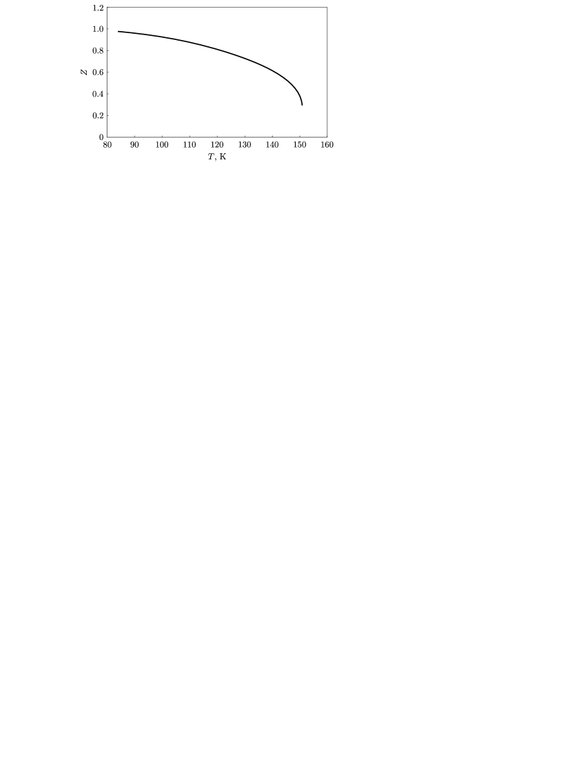
Figure 1: Thermodynamic properties of saturated argon. $Z$ is the compressibility factor, $Z=PV/kT$;   $T$ is the temperature in Kelvin degrees.

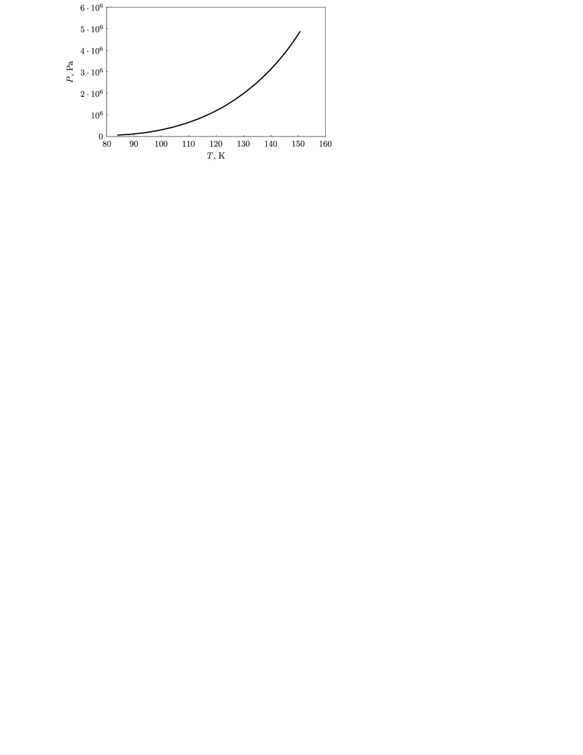
Figure 2: Thermodynamic properties of saturated argon. P is the pressure in pascals, T is the temperature in Kelvin degrees.

Thus, the formation of nanostructures in the other phase (the liquid one) plays a significant role, just as the formation of clusters in a gas.

Let us now pass to the case of a constant temperature (Fig. 3)[16].

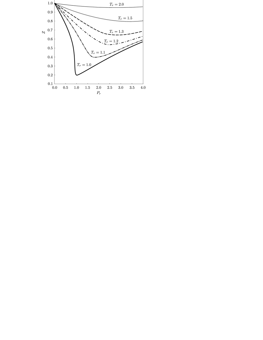
Figure 3: $T_{r}=T/T_{c}$, and $P_{r}=P/P_{c}$ are reduced temperature and pressure, respectively.

We can assume that, instead of $E$, $V^{2/3}$ tends to infinity. And hence, in all the formulas of Bose-Einstein type from [2], [3], we can assume that $b^{-1}\simeq\frac{V^{2/3}}{kT}$, where $T$ is the temperature, $k$ is the Boltzmann constant, and $d$ is the dimension. For the number $b$ in [17, 18] to be dimensionless, let us introduce the effective radius $a$ of the gas molecule (see below).

3 Taking into account the pair interactions between particles

Now consider the Hougen–Watson diagram given in Brushtein’s textbook “Molecular Physics” [25]. The diagram reflects the dependence of the compressibility factor $Z=PV/kTN$ on the pressure for different temperatures and was constructed by Hougen and Watson for seven gases: H₂, N₂, CO, NH₃, CH₄, C₃H₈, C₅H₁₂. Although the textbook states that attraction decreases compressibility, this, however, is obtained for Van-der-Waals gas under the condition $|1-Z|\ll 1$, i.e., time as a compressibility factor decreases down to $0{.}2$.

From our understanding of ideal gas, it follows from the distribution (2.1) that $Z$ can attain the value of $0{.}523$ and, further, the compressibility factor must decrease only at the expense of the interaction.

Phenomenological thermodynamics is based on the concept of pair interaction. Moreover, it is implicitly assumed that

there exists some one-particle distribution characterizing the field, to which all the particles contribute.

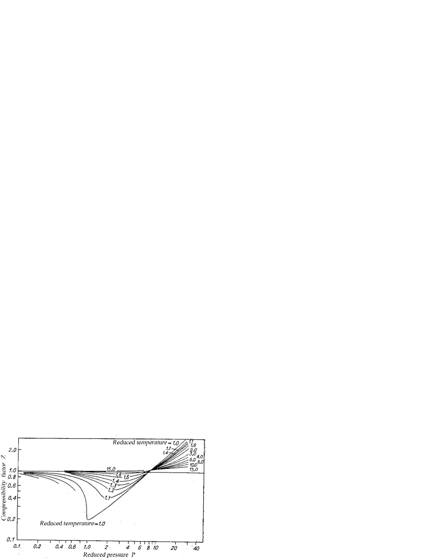
Figure 4: The original Hougen-Watson diagram.

They are interrelated. Formulas for the distribution corresponding to this mean field were rigorously obtained by the author in [26]. The equation that relates the potential of the mean field to pair interactions is called the equation of self-consistent (or mean) field. For the interaction potential $\Phi$, it is of the form

$$u(x,p)=u_{0}(x,p)+N\int\Phi(x-x^{\prime},p-p^{\prime})\frac{1}{e^{(p^{2}/2m+u(x^{\prime},p^{\prime}))(kT)^{-1}}-1}\,dx^{\prime}\,dp^{\prime}.$$ (3.1)

This equation was rigorously justified only in the case of long-range interaction, in particular, in [27].

In the case of a gas occupying the volume $V$ and not subject to the action of external forces, $u_{0}(x,p)=0$ for $x$ lying inside the volume $V$ and $u_{0}(x,p)=\infty$ on the boundary of this volume.

In what follows, we shall study only this case. For the interaction potential we take the Lennard-Jones potential or, for a greater coincidence with the experiment, the following potential:

$$\Phi(r)=\frac{\varepsilon n}{n-6}\biggl{(}\frac{n}{6}\biggr{)}^{6/(n-6)}\biggl{(}\frac{\sigma^{n}}{r^{n}}-\frac{\sigma^{6}}{r^{6}}\biggr{)}$$ (3.2)

containing one more parameter $n>6$.

In the zeroth approximation, as $\sigma\to 0$, the integral of the potential (3.1) with respect to $r$ from some $r_{0}$ to $\infty$. This integral substantially depends on $r_{0}$. How must we choose $r_{0}$?

Consider the scattering of one particle by another. Suppose that, as $t\to-\infty$, the velocities of the two colliding particles are equal to ${\bf{v}}_{1}^{in}$ and ${\bf{v}}_{2}^{in}$, respectively. This means that, at $t\to-\infty$ the trajectories of the particles approach straight lines. In terms of the variable $r=r_{2}-r_{1}$ as $t\to-\infty$ the radius vector of the $r$-point asymptotically approaches the function $r^{in}=\rho+{\bf{v}}^{in}t$, where $\rho{\bf{v}}^{in}=0$ and ${\bf{v}}^{in}={\bf{v}}^{in}_{2}-{\bf{v}}^{in}_{1}$. The constant vector $\rho$ is referred to as the target parameter. The quantity $\rho$ is equal to the distance between the straight lines along which the particles would move if no interaction was present. After the collision as $t\to\infty$, the velocities of the particles are equal to ${\bf{v}}_{1}^{out}$ and ${\bf{v}}_{2}^{out}$. This means that the radius vector $r(t)$ asymptotically approaches the function $r^{out}=c+{\bf{v}}^{out}t$. The trajectories $r^{in}(t)$ and $r^{out}(t)$, which are straight lines, are said to be the incoming and outgoing asymptotes. The value of the relative speed in the in- and out-states is preserved; namely, $|{\bf{v}}^{in}|=|{\bf{v}}^{out}|=v.$

The condition on the turning point $r_{0}$ is of the form

$$\left[\frac{v^{2}}{4}-\frac{(\rho v)^{2}}{2r^{2}}-\Phi(r)\right]=0.$$ (3.3)

Let is find the value of $\Phi(r)$ for the potential (3.1) (this value depends on $r_{0}$),

$$\widetilde{\Phi}(0)=\int^{\infty}_{r_{0}}\Phi(|r|)dr=4\varepsilon\int_{r_{0}}^{\infty}\left(\frac{\sigma^{12}}{r^{12}}-\frac{\sigma^{6}}{r^{6}}\right)dxdydz=\frac{16}{3}\pi\varepsilon\sigma^{3}\int^{\infty}_{r/\sigma}\left(\frac{1}{\xi^{10}}-\frac{1}{\xi^{4}}\right)d\xi=$$

$$=\frac{16\pi}{3}\varepsilon\sigma^{3}\left\{-\frac{1}{9}\left(\frac{\sigma}{r_{0}}\right)^{9}+\frac{1}{3}\left(\frac{\sigma}{r_{0}}\right)^{3}\right\}=\frac{16}{3}\pi\varepsilon\sigma^{3}\left(-\frac{1}{3}\frac{\sigma^{3}}{r^{3}_{0}}+\frac{1}{9}\frac{\sigma^{9}}{r_{0}^{9}}\right),$$ (3.4)

where $r/a=\xi$.

In particular, for $r_{0}=\sigma$, the area is equal to $-(8/9)\varepsilon\sigma^{3}\alpha$, where $\alpha=(4/3)p$. For $r_{0}=\frac{\sigma}{\sqrt[6]{3}}$, the area is equal to zero.

In the nanotube, the target parameter $\rho$ can be assumed to be zero. In this case,

$$\xi^{12}-\xi^{6}=\frac{p^{2}}{4\varepsilon m};\quad\xi=\frac{\sigma}{r_{0}}$$

$$\xi^{6}=x$$

$$x^{2}-x-\frac{p^{2}}{4\varepsilon m}=0$$

$$x_{1,2}=\frac{1}{2}+\sqrt{\frac{1}{4}+\frac{p^{2}}{4\varepsilon m}}=\frac{1}{2}+\frac{1}{2}\sqrt{1+\frac{p^{2}}{\varepsilon m}}.$$

$$\frac{\sigma}{r_{0}}=\left[\frac{1}{2}\left(1+\sqrt{1+\frac{p^{2}}{\varepsilon m}}\right)\right]^{1/6}$$ (3.5)

for $p=0,r_{0}=\sigma$.

The Lennard-Jones potential can now be represented in the form $\Phi(r_{0},r)=\Phi(r_{0}(p),r)$, and hence, since $|p|=|p_{i}-p_{j}|$, it follows that the equation for the dressed potential looks as follows:

$$u(p,x)=N\int\Phi(r_{0}(p-\eta),|x-\xi|)\frac{dpd\xi}{e^{\frac{b\eta^{2}}{2m}+u(\eta,\xi)}-1},\quad p\in R^{3},x\in R^{3}.$$ (3.6)

Since the external potential is absent and the distribution depends on $x$ in terms of the dressed potential only, we can assume that $u(p,x)=u(p)$ does not depend on $x$.

Making the change $x-\xi=y$ and integrating with respect to $y$ from $r_{0}$ to $\infty$, we obtain

$$u(p)=\frac{16}{3}\pi\varepsilon\sigma^{3}\int\frac{\frac{1}{9}\left[\frac{1}{2}+\frac{1}{2}\sqrt{1+\frac{(p-\eta)^{2}}{\varepsilon m}}\right]^{3/2}-\frac{1}{3}\left[\frac{1}{2}+\frac{1}{2}\sqrt{1+\frac{(p-\eta)^{2}}{\varepsilon m}}\right]^{1/2}}{e^{b\{\frac{\eta^{2}}{2m}-\mu+u(\eta)\}}-1}d\eta.$$ (3.7)

Here $\mu\leq 0$ stands for the chemical potential.

It should be noted that the probability of the event in which the particle $x_{2}$ occurs on the interval from $r_{0}$ to infinity is not constant. It is obviously proportional to the time during which the particle is kept within the interval ($x_{2}^{\prime},x_{2}^{\prime\prime}$), and this time is inversely proportional to the speed of $x_{2}$ with respect to the particle $x_{1}$. One can readily see that this probability is equal to

$$F(x_{2})=\frac{\left[\frac{1}{m}(p_{1}-p_{2})^{2}-\frac{\rho^{2}(p_{2}-p_{1})^{2}}{m(x_{2}-x_{1})^{2}}-\Phi(x_{2}-x_{1})\right]^{-1/2}-(\frac{1}{m}(p_{1}-p_{2})^{2})^{-1/2}}{\int_{r_{0}}^{\infty}\left\{\left[\frac{1}{m}(p_{1}-p_{2})^{2}-\frac{\rho^{2}(p_{2}-p_{1})^{2}}{m(x_{2}-x_{1})^{2}}-\Phi(x_{2}-x_{1})\right]^{-1/2}-(\frac{1}{m}(p_{1}-p_{2})^{2})^{-1/2}\right\}dr}.$$ (3.8)

Since the integral of the expression

$$\frac{F(x_{2})}{e^{b\{\frac{p_{2}^{2}}{m}+u(p_{2},\rho)-\mu\}}-1}\left[\int\left(e^{b\{\frac{p^{2}_{2}}{m}+u(p,\rho)-\mu\}}-1\right)^{-1}|p_{2}|^{2}dp_{2}\right]^{-1},$$

(first with respect to $x_{2}$ and then with respect to $dp$) is equal to one, it follows that the probabilities are independent, and the distribution with respect to $x_{2}$ and $p_{2}$ is equal to the product of the distributions with respect to $x_{2}$ and to $p_{2}$.

Let us find the energy level below which the “condensate” appears.

As is well known, the “turning point” $r_{0}$, the energy $E=m(v_{1}-v_{2})^{2}$, where $v_{1}$ and $v_{2}$ are the velocities of two interacting particles, and the impact parameter $\rho$ are related by

$$E-\frac{E\rho^{2}}{r_{0}^{2}}-\Phi(r_{0})=0.$$ (3.9)

1. The potential has the form $-\alpha/r^{4}$. Then the turning point $r_{0}$ in the scattering problem is defined by the relation

$$1-\frac{\rho^{2}}{r^{2}_{0}}+\frac{\alpha}{r^{4}E}=0,$$

where $E=(p_{1}-p_{2})^{2}/m$ is the energy of the particles an infinite distance apart and $\rho$ is the impact parameter. Hence

$$r_{0}=\frac{\rho^{2}}{2}+\sqrt{\frac{\rho^{4}}{4}-\frac{\alpha}{E}}\mspace{2.0mu},$$

and the solution is only possible if $E$ is bounded below: $E\geq 4\alpha/\rho^{4}$.

For $E=4\alpha/b^{4}$, we have the expression

$$1-\frac{b^{2}}{r^{2}}+\frac{\alpha}{r^{4}E}=\biggl{(}1-\frac{\rho^{2}}{2r}\biggr{)}^{2}>0$$

where $r>\rho^{2}/2$.

2. Suppose that the attraction potential is of the form

$$\Phi(r)=-4U_{0}\mspace{1.0mu}\frac{\sigma^{6}}{r^{6}}\,,\qquad E_{\min}=\min E=4U_{0}\sigma^{6}\max_{r_{0}<\rho}\frac{1}{r_{0}^{6}}\biggl{(}\frac{\rho^{2}}{r_{0}^{2}}-1\biggr{)}^{-1}=27U_{0}\mspace{1.0mu}\frac{\sigma^{6}}{\rho^{6}}\,.$$

Then we obtain

$$\frac{\Phi(r)}{E_{\min}}=-\frac{4}{27}\cdot\frac{\rho^{6}}{r^{6}}\,.$$

Note that, for $E<E_{\min}$, if there is no term corresponding to repulsion, then the “falling on the center” phenomenon occurs, i.e., the binding-together of the particles.

3. For the function

$$\Phi=4U_{0}\biggl{(}\frac{\sigma^{6}}{r^{6}}-\frac{\sigma^{12}}{r^{12}}\biggr{)}\biggl{(}\frac{\rho^{2}}{r^{2}}-1\biggr{)}^{-1},$$

the equation for extremum points is of the form

$$\Phi^{\prime}(x)=8\varepsilon\sigma^{6}\mspace{1.0mu}\frac{3x^{8}-2\rho^{2}x^{6}-6\sigma^{6}x^{2}+5\sigma^{6}\rho^{2}}{x^{11}(-\rho+x)^{2}(x+\rho)^{2}}=0\qquad x=r_{0}.$$

The graph of $\Phi(r_{0})$ for the given impact parameter $\rho=2\sigma$ is shown in Fig. 5.

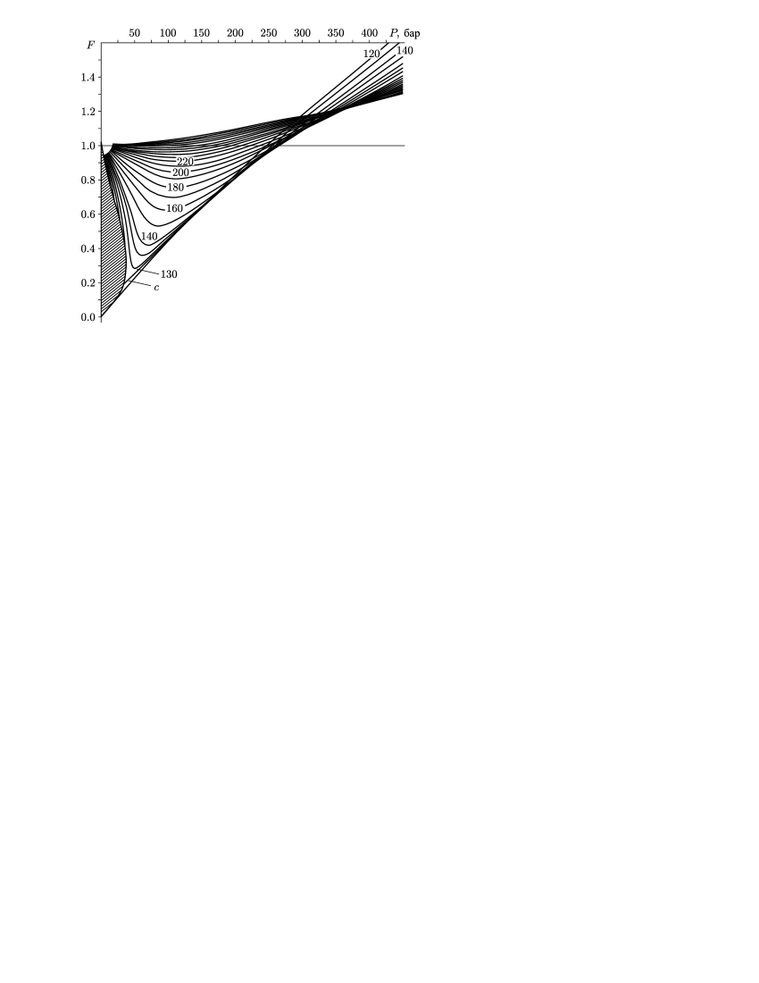
Figure 5: The Hougen-Watson diagram for nitrogen; $c$ is the critical temperature.

For $E$ less than some value of $E_{0}$, there appears a barrier whose the depth is $E_{\max}^{\text{loc}}-E_{\min}^{\text{loc}}$ and for which the probabilities of penetration of particles into the well [1], [28] due to thermal noise at a given temperature are well known. This implies that, below this barrier, the distributions that were obtained earlier for an ideal gas are false, because there exists a probability of penetration through the barrier at a given temperature. Thus, the maximum of the barrier is the natural minimum for the energy $(p_{1}-p_{2})^{2}/m$, below which we cannot use the distribution given above.

In [1], [28], it was calculated how much time a particle stays in a well of height $h$ and depth $\delta$ at a given temperature (thermal noise). If the number of particles $N$ tends to infinity, then this time is proportional to the number of particles occupying the well. It is a strange fact that this is in agreement with our estimates [11] of penetration into the condensate and yields the value $E_{\min}(\rho)$ for the condensate; for a given impact parameter $\rho$, this value corresponds to the same turning point $r_{0}\cong 1{.}21$ for the Lennard-Jones potential with $n=12$, to $r_{0}=1{.}02$ with $n=18$, and to $r_{0}=1{.}28$ with $n=7$.

But since $\rho^{3}$ for an ideal gas is of the order of $2V_{\text{sp}}\gg\rho^{3}$, then, accordingly, we can also define $E_{\min}$ from Eq. (3.9) for prescribed values of $r_{0}$ and $\rho=\sqrt[3]{2V_{\text{sp}}}$; $E_{\min}$ corresponds to the gases for which the interaction between particles is best described by the Lennard-Jones potential with a given $n$. If this is known, then $E_{\min}$ can be determined in terms of $V_{\text{sp}}$.

Using ${\mathcal{P}}_{\rho}((p_{1}-p_{2})^{2}/m)$, we define the one-dimensional distribution of the difference of the momenta in the scattering problem [14], [29]

$${\mathcal{P}}_{\rho}\biggl{(}\frac{(p_{1}-p_{2})^{2}}{m}\biggr{)}=\frac{1}{e^{(p_{1}-p_{2})^{2}/mkT-\mu^{\prime}/kT}-1}\biggl{(}\int_{p_{\min}}^{\infty}\frac{d\xi}{e^{\xi^{2}/mkT-\mu^{\prime}/kT}-1}\biggr{)}^{-1}.$$ (3.10)

Here $\rho_{\min}=\sqrt{mE_{\min}}$, and, as pointed out above, $E_{\min}$ is defined for the scattering problem by an interaction in the form of the Lennard-Jones potential.

The distribution (3.1) contains the chemical potential $\mu_{1}$ which is related to the chemical potential $\mu$ for the distribution with a “dressed” potential by relation (3.11) below, which expresses the fact that, for a fixed scattering parameter $\rho$, the number of particles in the one-dimensional scattering problem is of the order of $\sqrt[3]{N/2}$, where $N$ is the total number of particles outside the condensate.

The dressed potential $u$ depends on the three-dimensional momentum $p$ and is independent of the coordinates under the reduction to the scattering problem [26]. Therefore, the chemical potential $\mu_{1}$ is connected to the chemical potential $\mu=\mu(\rho)$ of the problem on the distribution with a dressed potential by the relation

$$\frac{2}{3}\mspace{1.0mu}\pi\int\frac{p^{2}\,dp}{e^{(p^{2}/2m+u(p,\rho)-\mu)/kT}-1}=\biggl{(}\int_{p_{\min}}^{\infty}\frac{dp}{e^{p^{2}/mkT-\mu_{1}/kT}-1}\biggr{)}^{3}.$$ (3.11)

If $u(p)$ is positive, then $p_{\min}=0$, and hence $\mu_{1}<0$.

In the integral equation of the mean field (3.1), we can drop the external potential $u_{0}$, because it is zero inside the volume, and finally obtain [26]

$$u(p,\rho)+C(\mu,\rho) =\frac{8}{9}\mspace{1.0mu}\pi^{2}\mspace{1.0mu}\frac{N}{V}\int_{0}^{\infty}\biggl{[}\int^{\infty}_{r_{0}(1/E,\rho)}\frac{\Phi(r)r^{2}\,dr}{\sqrt{1-\rho^{2}/r^{2}-\Phi(r)/E}}$$

$$\hphantom{{}=\frac{8}{9}\mspace{1.0mu}\pi^{2}\mspace{1.0mu}\frac{N}{V}\int_{0}^{\infty}\biggl{[}}\quad\quad\times\biggl{[}\int^{\infty}_{r_{0}}\biggl{\{}\biggl{(}\sqrt{1-\frac{\rho^{2}}{r^{2}}-\frac{\Phi(r)}{E}}\biggr{)}^{-1}-1\biggr{\}}\,dr\biggr{]}^{-1}$$

$$\hphantom{{}=\frac{8}{9}\mspace{1.0mu}\pi^{2}\mspace{1.0mu}\frac{N}{V}\int_{0}^{\infty}\biggl{[}}\quad\quad\times\frac{1}{e^{((p^{\prime})^{2}/2m+u(p^{\prime},\rho)-\mu)/kT}-1}$$

$$\hphantom{{}=\frac{8}{9}\mspace{1.0mu}\pi^{2}\mspace{1.0mu}\frac{N}{V}\int_{0}^{\infty}\biggl{[}}\quad\quad\times\frac{1}{e^{((p-p^{\prime})^{2}/m-\mu_{1})/kT}-1}(p^{\prime})^{2}\,dp^{\prime}\biggr{]}$$

$$\qquad\qquad\times\biggl{\{}\int^{\infty}_{p_{\min}}\frac{dp}{e^{(p^{2}/m-\mu_{1})/kT}-1}\biggr{\}}^{-4},$$ (3.12)

where $V$ is the volume, $r_{0}=r_{0}(\rho,E)$, and $E=(p-p^{\prime})^{2}/m$.

As presented in [26],

$$Z=\frac{2}{3kTV_{\text{sp}}^{2/3}}\int_{0}^{V_{\text{sp}}^{1/3}}\rho\,d\rho\,\int\biggl{\{}\frac{p^{2}}{2m}+u(p,\rho)\biggr{\}}\cdot\frac{p^{2}}{2m}\frac{p^{2}dp}{e^{p^{2}/2m+u(p,\rho)-\mu/kT}-1}\cdot\biggl{\{}\int\frac{p^{2}dp}{e^{p^{2}/2m+u(p,\rho)-\mu/kT}-1}\biggr{\}}^{-1}.$$ (3.13)

When the scattering problem is considered in the whole space, then the distribution over the scattering section is uniform. But we restrict the problem by the volume $V_{\text{sp}}$. Then there is no uniformity due to the boundary, at least, outside the domain, where

$$\frac{dZ}{dV_{\text{sp}}}<\frac{Z}{V_{\text{sp}}}\,.$$

Under different assumptions, the distribution $\mathcal{P}(\rho)$ over $\rho$ can be different (see [30] (the Bertrand paradox), [31], [32]). Moreover, $Z$ is described by an expression of type (3.13), averaged with respect to the distribution $\mathcal{P}(\rho)$ of the lines $\rho$ apart in the ball of radius $\sqrt[3]{V_{\text{sp}}}$.

$$Z=\frac{2}{3kTV_{\text{sp}}^{2/3}}\int_{0}^{V_{\text{sp}}^{1/3}}{\mathcal{P}(\rho)}\rho\,d\rho\,\int\biggl{\{}\frac{p^{2}}{2m}+u(p,\rho)\biggr{\}}\cdot\frac{p^{2}dp}{e^{p^{2}/2m+u(p,\rho)-\mu/kT}-1}\cdot\biggl{\{}\int\frac{p^{2}dp}{e^{p^{2}/2m+u(p,\rho)-\mu/kT}-1}\biggr{\}}^{-1},$$ (3.14)

where $\mu=\mu(\rho)$. Therefore, $Z$ can be taken at some mean point $\rho_{\text{mean}}(T,V_{\text{sp}})$. Then

$$\frac{dZ}{dV_{\text{sp}}}=\frac{dZ}{d\rho_{\text{mean}}}\cdot\frac{d\rho_{\text{mean}}}{dV_{\text{sp}}}=-\infty$$,

and hence,

$$\frac{dZ}{d\rho_{\text{mean}}}=-\infty$$.

If, at this point, the asymptotics as $p\to 0$ of $u(p,\rho_{\text{mean}})$ is of the form $-p^{2}/2m+\alpha(\rho_{\text{mean}})|\ln p|$, where $d\alpha/d\rho_{\text{mean}}>0$, then this leads to the domain in which $dZ/d\rho_{\text{mean}}=-\infty$, defining the $\lambda$-transition to the condensate state and to the law

$$\frac{dZ}{dP}=\frac{V_{\text{sp}}}{kT}$$

for $P>P_{\lambda}$ and $V_{\text{sp}}>V_{\lambda}$ ($P_{\lambda}$ and $V_{\lambda}$ depend on $T$).

The equation for the dressed potential is of the form (we have omitted the chemical potential for simplicity)

$$u(p,\rho)=\int_{0}^{\infty}\frac{F((p-\eta)^{2})\Theta((p-\eta)^{2})\eta^{2}\,d\eta}{e^{(p^{2}/2m+u(\eta,\rho))/kT}-1}\cdot\biggl{\{}\int^{\infty}_{p_{\min}}\frac{dp}{e^{p^{2}/mkT}-1}\biggr{\}}^{-4}-C,$$ (3.15)

where

$$F(mE) =\frac{8}{9}\frac{\pi^{2}}{\rho^{3}}\int^{\infty}_{r_{0}(1/E,\rho)}\frac{\Phi(r)r^{2}\,dr}{\sqrt{1-\rho^{2}/r^{2}-\Phi(r)/E}}$$

$$\qquad\qquad\times\biggl{[}\int^{\infty}_{r_{0}}\biggl{\{}\biggl{(}\sqrt{1-\frac{\rho^{2}}{r^{2}}-\frac{\Phi(r)}{E}}\biggr{)}^{-1}-1\biggr{\}}\,dr\biggr{]}^{-1}\cdot\frac{1}{e^{E/kT}-1}\,,$$ (3.16)

$\Theta((p-\eta)^{2})$ is nonzero only in the domain $|p-p^{\prime}|^{2}/m\geq E_{\min}$, $\rho^{3}=V_{\text{sp}}$, and $C=C(\mu,\rho)$.

Let us rewrite this equation in the form

$$u(p,\rho)=\frac{1}{2}\int_{-\infty}^{\infty}\frac{F((p-\eta)^{2})\Theta((p-\eta)^{2})\eta^{2}\,d\eta}{e^{(\eta^{2}/2m+u(\eta,\rho))/kT}-1}\cdot\biggl{\{}\int^{\infty}_{p_{\min}}\frac{dp}{e^{p^{2}/mkT}-1}\biggr{\}}^{-4}-C$$ (3.17)

and make the replacement $(p-\eta)^{2}=\xi^{2}$.

Then

$$u(p,\rho) =\frac{1}{2}\biggl{\{}\int_{\sqrt{mE_{\min}}}^{\infty}\frac{F(\xi^{2})\,d\xi}{e^{(\eta^{2}/2m+u(\eta,\rho))/kT}-1}+\int^{\sqrt{mE_{\min}}}_{-\infty}\frac{F(\xi^{2})\,d\xi}{e^{(\eta^{2}/2m+u(\eta,\rho))/kT}-1}\biggr{\}}$$

$$\qquad\qquad\times\biggl{\{}\int^{\infty}_{p_{\min}}\frac{dp}{e^{p^{2}/mkT}-1}\biggr{\}}^{-4}-C.$$ (3.18)

We search for conditions under which the solution of this equation, as $p\to\infty$, is of the form

$$u(p,\rho)=-\frac{p^{2}}{2m}+c(\rho),$$

where $dc/d\rho>0$.

First, note that, by virtue of proofs and estimates similar to those given in the theorems, we put the upper limit of the integral over $\eta$ equal to infinity, because $E$ in (1.11), (1.13), (1.15) (which is different from $E=(p-p^{\prime})^{2}/m$ in the scattering problem) is large, while the integrand is rapidly decaying, and the difference between the limit $\sqrt{2mE}$ and $\infty$ is less than the given estimates.

But since we are concerned with the asymptotics of the solution $u(p,\rho)$ as $p\to\infty$, it follows that, as $p^{\prime}\to\infty$, the integral over $p^{\prime}$ must sufficiently rapidly converge. Therefore, this remark must be taken into account only for some exotic family of solutions.

After the replacement indicated above, we express the term $\eta^{2}$ as $\eta^{2}=(\xi-p)^{2}$. But since the function is symmetric, it follows that the integration of $2p\xi$ over $\xi$ yields zero. Thus, we find that the term on the right-hand side of Eq. (3.15) is proportional to $p^{2}$. Now it suffices to equate the integral over $\xi$ as $p\to\infty$ to $-p^{2}/2m$. Moreover, the choice of the constant $c(\rho_{\text{mean}})$ remains arbitrary.

After the replacement, we obtain

$$u(p,\rho)=-\frac{p^{2}}{2m}+w(p,\rho);$$

here, as $p\to\infty$, we have $w(p,\rho)=c(\rho)|\ln p|$, and we can write an equation for the function $w(p,\rho)>0$, $dc(\rho_{\text{mean}})/d\rho_{\text{mean}}>0$. Moreover, the phase $\lambda$-transition, just as the minimal point of the condensate, depends on the power of the repulsive term in the Lennard-Jones potential as well on the quotients $\gamma=\sigma/V_{\text{sp}}^{1/3}$ and $\alpha=U_{0}/kT$. The points $\gamma_{\text{crit}}$ and the minimal point $\alpha$, corresponding to $dZ/dV_{\text{sp}}=-\infty$ are called $\lambda$-critical. As the pressure $w(p,\rho)$ increases above the point of the $\lambda$-transition, $V_{\text{sp}}$ remains unchanged. This implies that the volume $V$ decreases as the pressure increases, but, simultaneously, the number of particles outside the Bose condensate also decreases. It is possible that all the particles became dimers. and hence the total number of particles has decreased. Further, they all became trimers, etc. The volume $V$ has decreased, while the specific volume $V_{\text{sp}}$ remained constant—this is the law of the Bose condensate for classical gases or, more precisely, is the law of cluster formation.

The energy of the $\lambda$-point of the logarithmical form appears as $T=T_{\text{cr}}$. As one can see in Fig. 5 and by virtue of

$$\frac{dp}{dV_{\text{sp}}}|_{T=T_{\text{cr}},p=p_{\text{cr}}}=\frac{d^{2}p}{dV^{2}_{\text{sp}}}|_{T=T_{\text{cr}},p=p_{\text{cr}}}=0$$

the coefficient of incompressibility $\kappa=-(\partial\ln V_{\text{sp}})/\partial p$ turns to infinity, and the compressibility factor decreases steeply. This arouses a wave of compressibility (a shock wave), and therefore an additional term $c|p|$, where $c$ is the speed of sound, must occur in energy.

This term for $u(p,\rho)$ slows down the decrease of $Z$, and equation  (3.25) eliminates the shock wave as well as this term. At that instant for the derivative of heat capacity the so-called $\lambda$-point occurs. This effect is shown more obviously in Fig. 3.

This phenomenon, as well as consequences of the Pontryagin–Andronov–Vitt theorem, does not follow from classical mechanics but occurs when noise and fluctuations are taken into account. Therefore it does not follow from formulas for the dressed potential, although the equations of “collective oscillations,” as well as “equations of variations,” are related to the dressed potential [33, 34].

To illustrate this we use both wave and quantum equations. The wave equation of sound propagation has the form

$$\frac{\partial^{2}\Psi}{\partial t^{2}}=c^{2}\Delta\Psi,$$

whereas the Schrödinger equation is

$$ih\frac{\partial\Psi}{\partial t}=\left\{-\frac{h^{2}}{2m}\Delta+u(x)\right\}\Psi;$$ (3.19)

or in the iterated form

$$-h^{2}\frac{\partial^{2}\Psi}{\partial t^{2}}=\left\{-\frac{h^{2}}{2m}\Delta+u(x)\right\}^{2}\Psi.$$ (3.20)

As follows from formula (25) [34] and [35],

$$h^{2}\frac{\partial^{2}\Psi}{\partial t^{2}}=h^{2}c^{2}\Delta\Psi-\left\{-\frac{h^{2}}{2m}\Delta+u(x)\right\}^{2}\Psi+\widehat{O}(h^{2})\Psi,$$ (3.21)

where $\widehat{O}(h^{2})$ is an operator such that $\widehat{O}e^{S(x,t)/h}=O(h^{2})$ for any $C^{\infty}$-smooth $S(x,t)$.

For $u(x)=0$ and $\Psi=e^{(i/h)(px-Et)}$ this implies

$$E^{2}=c^{2}p^{2}+\frac{p^{4}}{4m^{2}},$$ (3.22)

which coincides with the spectrum obtained by N.N. Bogolyubov for the weakly nonideal classical gas [37]. This author has established in 1995 that this spectrum has quasiclassical rather than quantum nature [33, 34] and, based on a dependence from the capillary radius derived in [38], applied these results to the classical gas in nanotubes [39]. These predictions are justified by authoritative experimental data [40].

The phase-space boxes (1.23) are chosen to be invariant with respect to the Hamiltonian system corresponding to the Hamiltonian function $H(p,q)$. In the context of quantum chaos [21, 41], this corresponds to a kind of generalized ergodicity. Moreover, it follows from [33, 34, 35, 36] that the Hamiltonian

$$\sqrt{c^{2}p^{2}+H^{2}(p,q)}$$ (3.23)

corresponds to the Arnol’d diffusion in a self-consistent field.

In this case, the equation for the dressed potential has the form

$$u(p,\rho)+C(\mu,\rho) =\frac{4}{3}\mspace{1.0mu}\pi\mspace{1.0mu}\frac{1}{V_{\text{sp}}}\int_{0}^{\infty}\biggl{[}\int^{\infty}_{r_{0}(E,\rho)}\frac{\Phi(r)r^{2}\,dr}{\sqrt{1-\rho^{2}/r^{2}-\Phi(r)/E}}$$

$$\hphantom{{}=\frac{8}{9}\mspace{1.0mu}\pi^{2}\mspace{1.0mu}\frac{N}{V}\int_{0}^{\infty}\biggl{[}}\quad\quad\times\biggl{[}\int^{\infty}_{r_{0}(E,\rho)}\biggl{\{}\biggl{(}\sqrt{1-\frac{\rho^{2}}{r^{2}}-\frac{\Phi(r)}{E}}\biggr{)}^{-1}-1\biggr{\}}\,dr\biggr{]}^{-1}$$

$$\hphantom{{}=\frac{8}{9}\mspace{1.0mu}\pi^{2}\mspace{1.0mu}\frac{N}{V}\int_{0}^{\infty}\biggl{[}}\quad\quad\times\frac{1}{\exp((\sqrt{cp^{{}^{\prime}2}+p^{{}^{\prime}4}/4m^{2}}+u(p^{\prime},\rho))/kT)-1}$$

$$\hphantom{{}=\frac{8}{9}\mspace{1.0mu}\pi^{2}\mspace{1.0mu}\frac{N}{V}\int_{0}^{\infty}\biggl{[}}\quad\quad\times\frac{1}{\exp(((p-p^{\prime})^{2}/m-\mu_{1})/kT)-1}(p^{\prime})^{2}\,dp^{\prime}\biggr{]}$$

$$\qquad\qquad\times\biggl{\{}\int^{\infty}_{p_{\min}}\frac{dp}{\exp((p^{2}/m)/kT)-1}\biggr{\}}^{-3}$$ (3.24)

$$\qquad\qquad\times\biggl{(}\int\frac{p^{2}\,dp}{\exp((\sqrt{cp^{{}^{\prime}2}+p^{{}^{\prime}4}/4m^{2}}+u(p,\rho))/kT)-1}\biggr{)}^{-1},$$ (3.25)

where $\mu$ and $\rho$ are given, $C(\mu,\rho)$ is a constant depending on $\mu$ and $\rho$, $V_{\text{sp}}$ is the specific volume, $r_{0}=r_{0}(\rho,E)$, and $p_{\min}$ is determined by condition (3.11) for $\mu_{1}=\mu=0$.

After the change of variable $w(p,\rho)=u(p,\rho_{\text{mean}})-c|p|$ we find the values of $T$ and $V_{\text{sp}}$ for which $w(p,\rho_{\text{mean}})\approx O(p^{3})$ as $\mu(\rho_{\text{mean}})\to 0$.

It follows from the above theorems that as $N\to\infty$, it is necessary to introduce a parameter $\kappa$ in the exponential in (3.11) in the left-hand side and a parameter $\kappa_{1}$ in the exponential in the right-hand side. Since $p_{\min}\to 0$, we have $\kappa_{1}\gg\kappa$, and hence the kernel of the integral operator tends to the $\delta$-functoin as $\kappa\to 0$: $\delta(p-p^{\prime}+p_{\min})$. To cancel the term $\frac{|p|}{c}$ in the right-hand side as $p\to 0$, it is necessary to satisfy the relation between $p_{\min}$ and $\rho_{\text{mean}}$.

Then the leading term of the $T$ derivative of $TZ$, which contains the heat capacity $C_{v}$, will feature a logarithmic dependence characteristic for a $\lambda$ point. Indeed, as $\mu(\rho_{\text{mean}})\to 0$ we have

$$\int\frac{O(p^{3},\rho_{\text{mean}})p^{2}\,dp}{(e^{O(p^{3},\rho_{\text{mean}})}-1)^{2}}\sim\int\frac{dp}{p}.$$ (3.26)

Observe that although the quantum equations for the self-consistent field go over into the classical ones as $h\to 0$, the equations of variations for the quantum mechanical equations of the self-consistent field assume in the same limit an extra term with respect to the classical equations of variations (the equations of collective oscillations, see [39, 1.1]). This gives rise to the Hamiltonian (3.23).

One can assume that at temperatures below the $\lambda$ point ergodicity turns over into a KAM situation, making supefluidity of a classical gas possible in a very thin nanotube capillary. Thus the temperature of the $\lambda$ point can be regarded as the crossover point between the generalized ergodicity and the KAM dynamics.

References

• [1] L.S.Pontryagin, A.A.Andronov, and A.A.Vitt, On statistical consideration of dynamical systems. Zh. Γ‰xper. Teoret. Fiz. 3: 165-180 (1933)
• [2] L.D.Landau and E.M.Lifsihts. Statistical Physics. Nauka, Moscow, 1964. Pergamon Press, Oxford-Edinburgh-New York, 1968
• [3] V.A.Alekseev. Distributon Function of the Number of Particles in the Condensate of an Ideal Bose Gas Confined by a Trap. Zh. Γ‰xper. Teoret. Fiz. 119 (4): 700-709 (2001) J. Experiment. Theoret.Phys. 92 (4): 608-616 (2001)
• [4] A.N.Shiryaev. Probability. Nauka, Moscow, 1989; Springer-Verlag, New York, 1984.
• [5] V.V.Kozlov, Thermal equilibrium in the sense of Gibbs and PoincarΓ©. Institut Kompyut. Issled., Moscow–Izhevsk, 2002 [in Russian].
• [6] G.E.Andrews. The Theory of Partitions. Encyclopedia Math. Appl. Vol.Β 2. Addison–Wesley Publ., London, 1976.
• [7] A.M.Vershik. Statistical mechanics of combinatorial partitions, and their limit shapes. Funktsional. Anal. i Prilozhen. 30(2): 19–39 (1996) Functional Anal. Appl. 30(2): 90–105 (1996)].
• [8] V.P.Maslov, Quantum Linguistic Statistics. Russian J. Math. Phys. 13(3): 315–325 (2006).
• [9] V.P.Maslov and T.V.Maslova, On Zipf’s law and rank distributions in linguistics and semiotics. Mat. Zametki 80(5): 718–732 (2006) Math. Notes 80(5–6): 679–691 (2006).
• [10] V.P.Maslov, The Zipf-Mandelbrot law: quantization and an application to the stock market. Russian J. Math. Phys. 12(4): 483–488 (2005).
• [11] V.P.Maslov and V.E.Nazaikinskii, On the distribution of integer random variables related by two linear inequalities.Β I. Mat. Zametki 83(4): 559–580 (2008) Math. Notes 83(3–4): 512–529 (2008).
• [12] V.P.Maslov, Nonlinear averages in economics. Mat. Zametki 78(3): 377–395 (2005) Math. Notes 78(3–4): 347–363 (2005).
• [13] V.P.Maslov, New Look on the Thermodynamics of Gas and at Clusterizaton. Russian J. Math. Phys. 15(3): 494–511 (2008).
• [14] V.P.Maslov and V.E.Nazaikinskii, On the distribution of integer random variables related by a certain linear inequality.Β III. Mat. Zametki 83(6): 880–898 (2008) Math. Notes 83(5–6): 804–820 (2008).
• [15] V.P.Maslov, New concept of the nucleation process. Teoret. Mat. Fiz.156(1): 159–160 (2008) Theoret. and Math. Phys. 156(1): 1101–1102 (2008).
• [16] Compressibility factor. http://en.citizendium.org/wiki/Compressibility factor (gases),
• [17] V.P.Maslov. Solution of the Gibbs paradox in the framework of classical mechanics (Statistical Physics) and crystallization of the gas $C_{60}$. Mat. Zametki 83(5): 787–791 (2008) Math. Notes 83(5-6): 716?-722 (2008).
• [18] V.P.Maslov. Taking into account the interaction between particles in the new nucleation theory, quasiparticles, quantization of vortices, and the two-particle distribution function. Mat. Zametki 83(6): 864–879 (2008) Math. Notes 83(5-6): 790?-803 (2008).
• [19] R.D.Luce, E.U.Weber. An Axiomatic theory of conjoint, expected risk. Math. Psychology 30(2): 188–205 (1986)
• [20] V.P.Maslov. Quantum Economics Nauka, Moscow, 2006 [in Russian].
• [21] V.P.Maslov. Quantization of Thermodynamics and Ultrasecondary Quantization. Inst. Komp’yuternykh Issled,. Moscow, 2001 [in Russian].
• [22] A.N.Shiryaev. Fundamentals of Stochastic Financial Mathematics. Fazis, Moscow, 1998 [in Russian].
• [23] V.P.Maslov and V.E.Nazaikinskii, On the distribution of integer random variables related by a certain linear inequality, I. Mat. Zametki 83(2): 232–263 (2008) Math. Notes 83(2): 211–327 (2008).
• [24] V.P.Maslov and V.E.Nazaikinskii, On the distribution of integer random variables related by a certain linear inequality, II. Mat. Zametki 83(3): 381–401 (2008) Math. Notes 83(3): 345–363 (2008).
• [25] A.I.Burshtein, Molecular Physics Nauka, Novosibirsk, 1986 [in Russian].
• [26] V.P.Maslov, New Theory of nucleation. Russian J. Math. Phys. 15(3): 401–410 (2008).
• [27] V.P.Maslov and P.P.Mosolov, Asymptotic behavior as $N\rightarrow\infty$ of trajectories of $N$ point masses interacting according to Newton’s gravitation law. Izv. Akad. Nauk SSSR Ser.Mat. 42:(5), 1063–1100 (1978).
• [28] P.S.Landa. Theory of Fluctuational Transitions and Its Applications. J. Communications Technology and Electronics 46(10), 1068–1107 (2001).
• [29] V.P.Maslov and V.E.Nazaikinskii. On the distribution of integer random variables satisfying two linear relations. Mat. Zametki 84(1): 69–98 (2008) Math. Notes 84(1): 73–99 (2008).
• [30] J.Bertrand. Calcul des ProbabilitΓ©s. Gauthier-Villars, Paris, 1889.
• [31] R.V.Ambartsumyan, I.Mekke, and D.Shtoiyan, Introduction to Stochastic Geometry. Moscow, Nauka, 1989 [in Russian].
• [32] D.A.Klain and G.-C.Rota, Introduction to Geometric Probability. Cambridge Univ. Press, Cambridge, 1997.
• [33] V.P.Maslov. Quasi-Particles Associated with Lagrangian Manifolds Corresponding to Semiclassical Self-Consistent Fields. I. Russian J. Math. Phys. 2(4): 527-534 (1995)
• [34] V.P.Maslov. Quasi-Particles Associated with Lagrangian Manifolds Corresponding to Semiclassical Self-Consistent Fields. II. Russian J. Math. Phys. 3(1): 123-132 (1995)
• [35] V.P.Maslov. Quasi-Particles Associated with Lagrangian Manifolds Corresponding to Semiclassical Self-Consistent Fields. III. Russian J. Math. Phys. 3(2): 272-276 (1995)
• [36] V.P.Maslov. Uniforn asymptotics in the problem of superfluidity of classical liquid in nanotubes. ArXiv:0802.2650 [cond-mat.stat-mech] 19 Feb 2008
• [37] N.N.Bogolyubov. On the Theory of Superfluidity. Izvestia AN SSSR, ser. fizika 11 (1):77-90 (1947) [in Russian]
• [38] V.P.Maslov. Dependence of the superfluidity criterion on the capillary radius. Teoret. Mat. Fiz.143(3): 307-327 (2005) Theoret. and Math.Phys. 143(3): 741–759 (2005).
• [39] V.P.Maslov. Superfluidity of classical liquid in a nanotube for even and odd numbers of neutrons in a molecule. Teoret. Mat. Fiz.153(3): 388-408 (2007) Theoret. and Math.Phys. 153(3): 1677–1696 (2007).
• [40] G.Hummer, J.Rasaiah, J.Noworyta. Water conduction through the hydrophobic channel of a carbon nanotube. Nature, 414 (8), November: 188-190 (2001)
• [41] V.P.Maslov, A.S.Mishenko. Quasi-classical asymptotics of quasi-particles. Matematicheskii sbornik, 189(6): 85?116, 1998. [in Russian]