On the relation between $E(5)-$models and the interacting boson model

Abstract

The connections between the $E(5)-$models (the original $E(5)$ using an infinite square well, $E(5)-\beta^{4}$, $E(5)-\beta^{6}$ and $E(5)-\beta^{8}$), based on particular solutions of the geometrical Bohr Hamiltonian with $\gamma$-unstable potentials, and the interacting boson model (IBM) are explored. For that purpose, the general IBM Hamiltonian for the $U(5)-O(6)$ transition line is used and a numerical fit to the different $E(5)-$models energies is performed. It is shown that within the IBM one can reproduce very well all these $E(5)-$models. The agreement is the best for $E(5)-\beta^{4}$ and reduces when passing through $E(5)-\beta^{6}$, $E(5)-\beta^{8}$ and $E(5)$, where the worst agreement is obtained (although still very good for a restricted set of lowest lying states). The fitted IBM Hamiltonians correspond to energy surfaces close to those expected for the critical point.

1 Introduction

Both, the Bohr-Mottelson (BM) collective model bm and the interacting boson model (IBM) ibm have thoroughly been used to study the same kind of nuclear structure problems. Although very different in their formulation, the two models present clear relationships. Both models have three particular cases that can be easily solved and for which a clear correspondence can be done: i) spherical nucleus, ii) $\gamma$-unstable deformed rotor and, iii) axial rotor. For transitional situations and, specially in the phase transition areas, the correspondence between the two models is difficult Rowe05 . This suggests, for the case of transitional Hamiltonians, to look for the connection between BM and IBM through numerical studies.

In this work and in Ref. Garc08 , we concentrate on $E(5)$ and related models: the original $E(5)$ (infinite square well potential) Iach00 and, $E(5)$ with a potential $\beta^{4},\beta^{6}$ and, $\beta^{8}$, respectively Bona04 . All these models are produced in the BM scheme and a natural question is to ask for the corresponding equivalence in the IBM. Is the IBM able for producing the same spectra and transition rates? If yes, does the IBM Hamiltonian correspond to a critical point? This work is intended to answer these questions for those models and analyze the convergence as a function of the boson number. This procedure will allow to establish the IBM Hamiltonian which best fit the different $E(5)-$models and their relation with the critical points.

2 The IBM fit to $E(5)-$models

The most general, including up to two-body terms, IBM Hamiltonian can be written in multipolar form as,

$$\hat{H} = \varepsilon_{d}\hat{n}_{d}+\kappa_{0}\hat{P}^{\dagger}\hat{P}+\kappa_{1}\hat{L}\cdot\hat{L}+\kappa_{2}\hat{Q}\cdot\hat{Q}+\kappa_{3}\hat{T}_{3}\cdot\hat{T}_{3}+\kappa_{4}\hat{T}_{4}\cdot\hat{T}_{4}$$ (1)

where the definition of the different operators can be found in Ref. Fran94 .

The $E(5)-$models are intended to be of use for $\gamma$-unstable nuclei having $O(5)$ as symmetry algebra. For the construction of an IBM $\gamma$-unstable transitional Hamiltonian it is sufficient to impose in Eq. (1) $\kappa_{2}=0$. If additionally, we want to construct an IBM transitional Hamiltonian that preserves the $O(5)$ symmetry we have to impose the constraint $\kappa_{1}-\kappa_{3}/10-\kappa_{4}/14=0$ Garc08 . In practice, we do not impose the later restriction but, as it will be shown, this condition will be fulfilled in every fit. It is worth noting that in Ref. Garc08 we used the extra constraint $\kappa_{4}=0$ for simplicity and, the raised conclusions are qualitatively identical to the ones obtained in the present contribution.

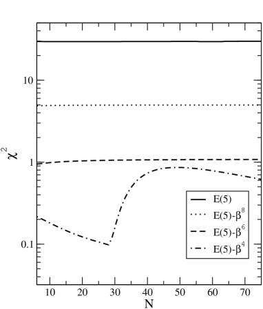
Figure 1: $\chi^{2}$ for the IBM fit to the energy levels of the different $E(5)$-models, as a function of $N$.

In order to perform the fit, we minimize a standard $\chi^{2}$ function for the energies, using $\varepsilon_{d}$, $\kappa_{0}$, $\kappa_{1}$, $\kappa_{3}$, and $\kappa_{4}$ as free parameters and $\kappa_{2}$ fixed to zero. We have done fits of the IBM Hamiltonian (1) parameters, as a function of $N$, so as to reproduce as well as possible the energies generated by the different $E(5)-$models (see Ref. Garc08 for more details about the fitting procedure). The value of the $\chi^{2}$ for a best fit to the different $E(5)-$models as a function of $N$ is shown in Fig. 1. It is clearly observed that for any $N$ the agreement between the fitted IBM and the $E(5)-\beta^{4}$ model is excellent and is getting worse for $E(5)-\beta^{6}$, $E(5)-\beta^{8}$, up to reach $E(5)$ which is the worst case. In particular $\chi^{2}(E(5)-\beta^{4})\approx\chi^{2}(E(5))/50$. It is worth noting that these results change slowly with the boson number and in all cases the $\chi^{2}$ value is approximately constant, except for $E(5)-\beta^{4}$ which is decreasing. If the calculations are extended till $N=1000$ bosons (see Ref. Garc08 ) one observes how $\chi^{2}$ values will continue having finite values, close to the ones given in figure 1, except for the case $E(5)-\beta^{4}$ which decreases and, it is expected to vanish for $N\rightarrow\infty$, as it was shown in Ref. Aria03 .

To have a clearer idea of the degree of agreement between the fitted IBM results with the data from the $E(5)-$models we analyze the case of $N=60$. In Table 1 we give the parameters of the Hamiltonian.

	$\varepsilon_{d}$	$\kappa_{0}$	$\kappa_{1}$	$\kappa_{3}$	$\kappa_{4}$
$E(5)$	251.84	0.16	23.5570	-16.6450	352.83
$E(5)-\beta^{8}$	1499.20	27.11	12.8750	4.0282	174.52
$E(5)-\beta^{6}$	2482.80	42.66	4.3049	10.1250	46.08
$E(5)-\beta^{4}$	2543.00	39.92	0.7143	6.2221	1.29

Table 1: Parameters of the IBM Hamiltonians used in table 2.

Note that the best fit parameters give rise approximately to the cancellation of the quadratic Casimir operator for $O(3)$, i.e. $\kappa_{1}-\kappa_{3}/10-\kappa_{4}/14=0$. This condition is approximately fulfilled for any number of bosons.

In Table 2 we present the value of the energies for $N=60$. The agreement for $E(5)-\beta^{4}$, $E(5)-\beta^{6}$, and $E(5)-\beta^{8}$ is really remarkable for all the states. Only in the case of $E(5)$, one can observe small discrepancies in the $\xi=2$ and $\xi=3$ bands, while for $\xi=1$ the agreement is perfect. This impressive one-to-one correspondence between the IBM and the $E(5)-$ states, at least for some bands, suggests the existence of an underlying phenomenon similar to the quasidynamical symmetry Rowe05 ; Rowe04a which is called quasi-critical point symmetry Garc08 .

Once the parameters of the Hamiltonian have been fixed we check the wave functions through the calculations of the relevant $B(E2)$ values. For all the cases, the agreement between the IBM calculations and the $E(5)-$ counterpart is reasonable Garc08 .

Another consequence of the excellent agreement between the $E(5)-$models and the IBM is that it is impossible to discriminate, from a experimental point of view, between a $E(5)-$model and its IBM counterpart.

	$\xi,\tau$	E(5)	IBM	E(5)-$\beta^{8}$	IBM	E(5)-$\beta^{6}$	IBM	E(5)-$\beta^{4}$	IBM
$0_{1}^{+}$	1,0	0.000	0.000	0.000	0.000	0.000	0.000	0.000	0.000
$2_{1}^{+}$	1,1	1.000	1.000	1.000	1.000	1.000	1.000	1.000	1.000
$4_{1}^{+}$	1,2	2.199	2.196	2.157	2.156	2.135	2.137	2.093	2.092
$2_{2}^{+}$	1,2	2.199	2.195	2.157	2.156	2.135	2.137	2.093	2.092
$0_{2}^{+}$	2,0	3.031	3.035	2.756	2.757	2.619	2.622	2.390	2.389
$6_{1}^{+}$	1,3	3.590	3.587	3.459	3.457	3.391	3.393	3.265	3.264
$4_{2}^{+}$	1,3	3.590	3.586	3.459	3.457	3.391	3.393	3.265	3.264
$3_{1}^{+}$	1,3	3.590	3.586	3.459	3.457	3.391	3.393	3.265	3.264
$0_{3}^{+}$	1,3	3.590	3.586	3.459	3.456	3.391	3.393	3.265	3.264
$2_{3}^{+}$	2,1	4.800	4.761	4.255	4.235	4.012	3.977	3.625	3.632
$6_{2}^{+}$	1,4	5.169	5.172	4.894	4.896	4.757	4.756	4.508	4.508
$5_{1}^{+}$	1,4	5.169	5.172	4.894	4.895	4.757	4.756	4.508	4.508
$4_{3}^{+}$	1,4	5.169	5.172	4.894	4.895	4.757	4.756	4.508	4.508
$2_{4}^{+}$	1,4	5.169	5.171	4.894	4.895	4.757	4.756	4.508	4.508
$4_{4}^{+}$	2,2	6.780	6.683	5.874	5.843	5.499	5.424	4.918	4.935
$2_{5}^{+}$	2,2	6.780	6.683	5.874	5.843	5.499	5.424	4.918	4.935
$0_{4}^{+}$	3,0	7.577	7.522	6.364	6.372	5.887	5.805	5.153	5.176
$2_{7}^{+}$	3,1	10.107	9.974	8.269	8.293	7.588	7.448	6.563	6.606

Table 2: Comparison of energy levels for fitted IBM Hamiltonians, with $N=60$, compared with those provided by the $E(5)$-models (see text).

3 The critical Hamiltonian

One of the most attractive features of the $E(5)-$models is that they are supposed to describe, at different approximation levels, the critical point in the transition from spherical to deformed $\gamma$-unstable shapes. Since they are connected to a given IBM Hamiltonian, as shown in the preceding section, this should correspond to the critical point in the transition from $U(5)$ to $O(6)$ IBM limits. Is this the case for the fitted IBM Hamiltonians obtained in the preceding section?

To analyze critical points and phase transitions in the IBM, one of the options is to use the intrinsic state formalism IF which introduces the shape variables $(\beta,\gamma)$ in the IBM. Due to the characteristics of the Hamiltonian we are working on, we can only observes second order phase transitions. To know if we have a critical Hamiltonian, it is convenient to use the concept of IBM “essential” parameters $(r_{1},r_{2})$ Lope96 , directly related with the parameters of the Hamiltonian (1), that allows to quantify the closeness to a critical point. In particular, in our case $r_{2}$ always vanishes (because $k_{2}=0$) while $r_{1}$ is defined as,

$$r_{1}=\frac{-\kappa_{0}+(\varepsilon_{d}+6\,\kappa_{1}+\frac{7}{5}\,\kappa_{3}+\frac{9}{5}\,\kappa_{4})/(N-1)}{\kappa_{0}+\frac{36}{35}\,\kappa_{4}+(\varepsilon_{d}+6\,\kappa_{1}+\frac{7}{5}\,\kappa_{3}+\frac{9}{5}\,\kappa_{3})/(N-1)}.$$ (2)

In this language, a critical Hamiltonian corresponds to $r_{1}=0$. In figure 2 the values of $r_{1}$ as a function of $N$ for the IBM Hamiltonians obtained from the fit are presented for the different studied $E(5)-$models. In all the cases it is observed an approximation to $r_{1}=0$ as the number of bosons increase. For the $E(5)-\beta^{4}$ model it is known that $r_{1}=0$ is reached for very large number of bosons Aria03 .

Figure 2: Values of $r_{1}$ (see text for definition) as a function of $N$ for the fitted IBM Hamiltonians.

4 Conclusions

In this paper, we have studied the connection between the $E(5)-$models and the IBM on the basis of a numerical mapping between both models. We have shown that it is possible, in all cases, to establish a one-to-one mapping between the $E(5)-$models and the IBM with a remarkable agreement for the energies and the $B(E2)$ values. Globally, the best agreement is obtained for the $E(5)-\beta^{4}$ Hamiltonian and the worst for the $E(5)$ case. All this suggests the presence of an underlying quasi-critical point symmetry Garc08 .

Another consequence of this excellent agreement is that it is impossible, from a experimental point of view, to discriminate between a $E(5)$-model and its corresponding IBM Hamiltonian when only few low-lying states are considered.

We have also proved that all the $E(5)-$models correspond to IBM Hamiltonians very close to the critical area, $|r_{1}|<0.05$. Therefore, one can say that the $E(5)-$models are appropriated to describe transitional $\gamma-$unstable regions close to the critical point.

References

- (1) A. Bohr, B.R. Mottelson, Nuclear Structure, vol. II, (Benjamin, Elmsford, NY, 1969).
- (2) F. Iachello and A. Arima, The interacting boson model (Cambridge University Press, Cambridge, 1987).
- (3) D.J. Rowe and G. Thiamanova, Nucl. Phys. A 760, 59 (2005).
- (4) J.E. García-Ramos and J.M. Arias, Phys. Rev. C 77, 054307 (2008).
- (5) F. Iachello, Phys. Rev. Lett. 85, 3580, (2000).
- (6) D. Bonatsos, D. Lenis, N. Minkov, P.P. Raychev, and P.A. Terziev. Phys. Rev. C 69, 044316 (2004).
- (7) A. Frank and P. Van Isacker, Algebraic Methods in Molecular and Nuclear Structure Physics (John Wiley & Sons, NY, 1994).
- (8) J.M. Arias, C.E. Alonso, A. Vitturi, J.E. García-Ramos, J. Dukelsky, and A. Frank, Phys. Rev. C 68, 041302(R) (2003); J.E. García-Ramos, J. Dukelsky, and J.M. Arias, Phys. Rev. C 72, 037301 (2005).
- (9) D.J. Rowe, Phys. Rev. Lett. 93, 122502 (2004).
- (10) J.N. Ginocchio, M.W. Kirson, Nucl. Phys. A 350, 31 (1980); A.E.L. Dieperink, O. Scholten, F. Iachello, Phys. Rev. Lett. 44, 1747 (1980); A.E.L. Dieperink and O. Scholten, Nucl. Phys. A 346, 125 (1980).
- (11) E. López-Moreno and O. Castaños, Phys. Rev. C 54, 2374, (1996).