On analyticity with respect to the replica number in random energy models II: zeros on the complex plane

Abstract

We characterize the breaking of analyticity with respect to the replica number which occurs in random energy models via the complex zeros of the moment of the partition function. We perturbatively evaluate the zeros in the vicinity of the transition point based on an exact expression of the moment of the partition function utilizing the steepest descent method, and examine an asymptotic form of the locus of the zeros as the system size tends to infinity. The incident angle of this locus indicates that analyticity breaking is analogous to a phase transition of the second order. We also evaluate the number of zeros utilizing the argument principle of complex analysis. The actual number of zeros calculated numerically for systems of finite size agrees fairly well with the analytical results.

1 Introduction

The replica method (RM) is a powerful tool in statistical mechanics for the analysis of disordered systems [1] . In general, the objective of RM is to evaluate the generating function

$$\phi_{N}(n)=\frac{1}{N}\log\left\langle Z^{n}\right\rangle,$$ (1)

for real replica numbers $n\in\mathbb{R}$ (or the complex field $\mathbb{C}$). Here, $Z$ is the partition function, $N$ represents the system size and $\left\langle\cdots\right\rangle$ denotes the configurational average with respect to the external randomness which governs the objective system. Direct evaluation of eq. (1) is generally difficult. However, eq. (1) can often be evaluated for natural numbers $n=1,2,\ldots\in\mathbb{N}$ in the thermodynamic limit as $N\to\infty$. Therefore, in RM, one usually evaluates

$$\phi(n)=\lim_{N\to\infty}\phi_{N}(n)$$ (2)

for $n\in\mathbb{N}$, in order to first obtain an analytic expression for $\phi(n)$ and then analytically continues this expression to $n\in\mathbb{R}$ (or $\mathbb{C}$).

There are two known possible problems with this procedure. The first problem is multiple possible alternatives for analytic continuation [2]. Even if all values of $\left\langle Z^{n}\right\rangle$ are provided for $n\in\mathbb{N}$, analytic continuation of $\phi_{N}(n)$ from $n\in\mathbb{N}$ to $n\in\mathbb{R}$ (or $\mathbb{C}$) is not uniquely determined. van Hemmen and Palmer conjectured that this may be the origin of the failure of the replica symmetric (RS) solution in the low temperature phase of the Sherrington-Kirkpatrick (SK) model [3]. The other issue is the possible breakdown of analyticity of $\phi(n)$. Although analyticity of $\left\langle Z^{n}\right\rangle$ with respect to $n$ is generally guaranteed as long as $N$ is finite, $\phi(n)=\lim_{N\to\infty}\phi_{N}(n)$ may fail to be analytic. This implies that if such a breaking of analyticity occurs at $n=n_{c}<1$, then continuing the expression analytically from $n\in\mathbb{N}$ to $n\in\mathbb{R}$ will lead to an incorrect solution for $n$ in the range of $n<n_{c}$.

In [4, 5], the authors developed an exact expression of the moment $\left<Z^{n}\right>$ for discrete versions of random energy models (DREMs) [6, 7]. The expression is valid for $n\in\mathbb{C}$ and is useful for handling systems of finite size. Utilizing this expression, it can be shown that analyticity breaking of $\phi(n)$ actually occurs at a certain critical replica number $n=n_{c}<1$ in the low temperature phase of DREMs. The uniqueness of the analytic continuation from $n\in\mathbb{N}$ to $n\in\mathbb{C}$ is guaranteed for DREMs. This means that the analyticity breaking of $\phi(n)$ with respect to $n$ is the origin of the one step replica symmetry breaking (1RSB) which is observed for DREMs, and thus we are motivated to further explore its mathematical structure.

This paper is written with this motivation in mind. Regarding $\log Z$ as the energy of the external randomness, the moment $\left\langle Z^{n}\right\rangle$ and generating function $\phi(n)$ are formally analogous to the partition function and free energy of non-random systems. This analogy leads us to characterize analyticity breaking in terms of the distribution of zeros of $\left\langle Z^{n}\right\rangle$ on the complex $n$ plane, following the argument by Lee and Yang [8, 9, 10, 11]. Let us suppose that a partition function of a finite size system is expressed as a function of a certain control parameter $\zeta$. As long as $\zeta$ is real, the partition function does not vanish. However, there can exist zero points, which are generally termed the Lee-Yang zeros, throughout the complex $\zeta$ plane. In general, the Lee-Yang zeros are apart from the real axis as long as the system size $N$ is finite. However, when a certain phase transition occurs at a critical parameter value $\zeta_{c}\in\mathbb{R}$, the distribution of the zeros becomes dense and approaches $\zeta_{c}$ as $N\to\infty$. The way in which this occurs characterizes the type of the phase transition. The main purpose of this paper is to apply such a description to the analyticity breaking of $\phi(n)$ by evaluating the zeros of $\left\langle Z^{n}\right\rangle$ on the complex plane of the replica number $n$.

This paper is organized as follows. In section 2, we briefly discuss the Lee-Yang zeros, utilizing a simple model. In section 3, which is the main part of this paper, we apply the Lee-Yang approach to examine the analyticity breaking of $\left\langle Z^{n}\right\rangle$ of DREM. The exact expression for $\left\langle Z^{n}\right\rangle$ developed in [4, 5] is utilized to perturbatively evaluate the zeros in the vicinity of the transition point employing the steepest descent method. This shows that the the distance of the closest zero to the real axis decays as $O(N^{-1/2})$ when the system size $N$ is large. In the thermodynamic limit as $N\to\infty$, the incident angle of the locus to the real axis converges to $\pi/4$, indicating that analyticity breaking is analogous to a phase transition of the second order. However, it is also shown that the angle between the real axis and the line connecting the transition point with the $k$th zero from the real axis has a finite positive correction from $\pi/4$ independently of $N$ as long as $k(=1,2,\ldots)$ is finite. The complex zeros are also numerically evaluated for several system sizes based on the expression, which is consistent with the asymptotic form to a reasonable precision. The final section is devoted to a summary.

2 Complex zeros and analyticity

2.1 Brief review of Lee-Yang zeros

Partition functions of discrete systems of finite size are, in general, analytic with respect to their parameters because they are a summation of exponents of the Hamiltonian over all possible (but still a finite number of) states. In addition, they do not have zeros on the real axis for the same reason.

A theorem by Weierstrass [12],

“There exists an entire function with arbitrarily prescribed zeros $a_{n}$ provided that, in the case of infinitely many zeros, $a_{n}\rightarrow\infty$. Every entire function with these and no other zeros can be written in the form

$$f(z)=z^{m}e^{g(z)}\prod_{n=1}^{\infty}(1-\frac{z}{a_{n}})e^{\frac{z}{a_{n}}+\frac{1}{2}(\frac{z}{a_{n}})^{2}+\cdots+\frac{1}{m_{n}}(\frac{z}{a_{n}})^{m_{n}}}$$ (3)

where the product is taken over all $a_{n}\neq 0$, the $m_{n}$ are certain integers, and $g(z)$ is an entire function.”,

indicates that a partition function $Z(\zeta)$ of a finite system can generally be expanded with respect to a parameter $\zeta$ as

$$Z(\zeta) = e^{g(\zeta)}\prod_{n=1}^{\infty}(1-\frac{\zeta}{a_{n}})e^{\frac{\zeta}{a_{n}}+\frac{1}{2}(\frac{\zeta}{a_{n}})^{2}+\cdots+\frac{1}{m_{n}}(\frac{\zeta}{a_{n}})^{m_{n}}},$$ (4)

where the ${a_{n}}$ are not on the real axis. Here, $\zeta$ may be the inverse of the temperature $\beta$, an external field, or any other parameters of the Hamiltonian. In most cases, partition functions are physically relevant only for real values of $\zeta$. Eq. (4) yields an expression for the free energy,

$$F(\zeta)=-\frac{C}{\beta}\log{Z(\zeta)}$$ (5)

$$=-\frac{C}{\beta}\left\{g(\zeta)+\sum_{n=1}^{\infty}\log{(1-\frac{\zeta}{a_{n}})}+\frac{\zeta}{a_{n}}+\frac{1}{2}(\frac{\zeta}{a_{n}})^{2}+\cdots+\frac{1}{m_{n}}(\frac{\zeta}{a_{n}})^{m_{n}}\right\}$$ (6)

where $\beta>0$ denotes the inverse temperature and $C$ is a constant with respect to $\zeta$, introduced so that the thermodynamic limit is well-defined. For systems of finite size, $F(\zeta)$ is analytic in a neighborhood of the real axis since the $a_{n}$ are located a finite distance away from the real axis. Therefore, systems of finite size do not exhibit phase transitions with respect to $\zeta$.

In the thermodynamic limit, however, the $a_{n}$ can become dense and may approach the real axis. In such cases, the summation of the logarithm in eq. (6) is replaced by an integral with an integral contour which intersects the real axis. As a consequence, the free energy is expressed by a different analytic function on each side of the integral contour. This implies that a phase transition occurs at the intersection point as $\zeta$ varies along the real axis.

2.2 Simple example

To illustrate the above scenario intuitively, we consider here a simple example. Let us suppose that the partition function of the example model can be written as,

$$Z(\zeta;a,\zeta_{c})=\cosh{\frac{\pi}{2a}(\zeta-\zeta_{c})}$$ (7)

where $a$ and $\zeta_{c}$ are real positive numbers. The free energy is then

$$F(\zeta;a,\zeta_{c})=-\frac{2a}{\beta}\log{Z(\zeta;a,\zeta_{c})}.$$ (8)

where $2a$ is introduced to make the thermodynamic limit of this model well-defined. Since $\cosh{z}\simeq e^{{\rm sign}({\rm Re}(z))z}/2$ for $|z|\gg 1$ holds , $Z(\zeta;a,\zeta_{c})$ behaves like

$$Z(\zeta;a\to 0,\zeta_{c})$$ (9)

$$\rightarrow\frac{1}{2}e^{\frac{\pi}{2a}(\zeta-\zeta_{c})}\Theta({\rm Re}(\zeta-\zeta_{c}))+\frac{1}{2}e^{-\frac{\pi}{2a}(\zeta-\zeta_{c})}\Theta(-{\rm Re}(\zeta-\zeta_{c})),$$ (10)

in the limit as $a\rightarrow 0$, where ${\rm sign}(x)=x/|x|$ for $x\neq 0$, and $\Theta(x)=1$ for $x>0$ and vanishes for $x<0$. ${\rm Re}(z)$ denotes the real part of a complex number $z$. This shows that the free energy can be expressed as

$$F(\zeta;a\to 0,\zeta_{c})=-\frac{\pi}{\beta}(\zeta-\zeta_{c})\{\Theta({\rm Re}(\zeta-\zeta_{c}))-\Theta(-{\rm Re}(\zeta-\zeta_{c}))\},$$ (11)

in this limit. This means that the analytic property of the free energy changes at the boundary ${\rm Re}(\zeta)=\zeta_{c}$; more precisely, the first derivative of $F(\zeta;a,\zeta_{c})$ with respect to $\zeta$ becomes discontinuous at ${\rm Re}(\zeta)=\zeta_{c}$ whereas the real part of the free energy remains continuous. If the parameter $\zeta$ is the temperature or an external field, this indicates that a first order phase transition occurs at $\zeta=\zeta_{c}$.

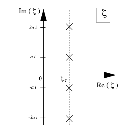
Figure 1: Zero points of the partition function $Z(\zeta;a,\zeta_{c})=\cosh{\frac{\pi}{2a}(\zeta-\zeta_{c})}$. They become dense and approach the real axis in the limit as $a\rightarrow 0$

This transition can be linked to the asymptotic behavior of zeros of $\zeta$ in the complex plane, which arises in the “artificial thermodynamic limit” as $a\to 0$, as follows. Using the product expansion of $\cosh{z}$,

$$\cosh{z}=\prod_{k=1}^{\infty}\left(1+\frac{4z^{2}}{(2k-1)^{2}\pi^{2}}\right),$$ (12)

we can write

$$Z(\zeta;a,\zeta_{c})=\prod_{k=1}^{\infty}\left(1+\frac{(\zeta-\zeta_{c})^{2}}{(2k-1)^{2}a^{2}}\right),$$ (13)

which implies that $g(\zeta)$ and $m_{n}$ are zero in the expression of eq.(4). Eq. (13) means that zeros of $Z(\zeta;a,\zeta_{c})$ do not occur on the real axis but are distributed on $\zeta=\zeta_{c}\pm(2k-1)a{\rm i}$ $(k=1,2,\ldots)$ as is depicted in figure 1, where ${\rm i}=\sqrt{-1}$. Therefore, the free energy of this model can be expressed as

$$F(\zeta;a,\zeta_{c})=-\frac{2a}{\beta}\sum_{k=1}^{\infty}\log{\left(1+\frac{(\zeta-\zeta_{c})^{2}}{(2k-1)^{2}a^{2}}\right)}.$$ (14)

All the zeros $\zeta=\zeta_{c}\pm(2k-1)a{\rm i}$ correspond to branch points of the logarithm. Nevertheless, the free energy is still analytic along the real axis as long as $a$ is finite since there are no branch points on the real axis.

However, the situation changes in the limit as $a\to 0$ since the distance of zeros from the real axis becomes infinitesimal. Actually, the summation has to be replaced by an integral thus:

$$F(\zeta;a\to 0,\zeta_{c})=-\frac{1}{\beta}\int_{0}^{\infty}dx\log{\left(1+\frac{(\zeta-\zeta_{c})^{2}}{x^{2}}\right)},$$ (15)

which implies that the integrand becomes singular at $x=|\zeta-\zeta_{c}|$ when ${\rm i}(\zeta-\zeta_{c})$ or $-{\rm i}(\zeta-\zeta_{c})$ is a non-negatie real number. As a consequence, this integral correctly reproduces eq. (11), which is singular along a line ${\rm C1}:\zeta=\zeta_{c}+v{\rm i}$ parameterized by $v\in\mathbb{R}$ including the real critical parameter $\zeta=\zeta_{c}$.

2.3 Remarks

Two issues are noteworthy here.

2.3.1 Argument principle and the number of zeros

The first issue concerns the number of zeros inside a closed contour. For any complex function $f(z)$ which is meromorphic inside a closed contour $\gamma$, the identity

$$\frac{1}{2\pi{\rm i}}\int_{\gamma}\frac{f^{\prime}(z)}{f(z)}dz=\sum_{j}n(\gamma,a_{j})-\sum_{k}n(\gamma,b_{k}),$$ (16)

holds, where $a_{j}$ and $b_{k}$ are the zeros and poles inside $\gamma$, respectively. $n(\gamma,p)$ represents the winding number of $\gamma$ around $p$. This formula is sometimes termed the argument principle [12]. Applying this to eqs. (4) and (6), one can evaluate the number of zeros in the region surrounded by $\gamma$ . In most cases, analytically finding all zeros is difficult and one has to resort to numerical schemes such as Newton’s method. A major difficulty of such approaches is to determine whether there has been a sufficient number of search trials. On the other hand, in some cases, the free energy density can be obtained in a computationally feasible manner in the thermodynamic limit. Therefore, one can estimate the asymptotic number of zeros by applying eq. (16) to the free energy density. This approach can be utilized to check whether or not sufficiently many zeros have been obtained.

2.3.2 Incident angle and type of phase transition

The second issue is the relation between the locus of the zeros and the type of the phase transition. In the simple model mentioned above, the locus that the zeros form in the limit as $a\to 0$ is the straight line ${\rm C1}:\zeta=\zeta_{c}+v{\rm i}$ $(v\in\mathbb{R})$, which is perpendicular to the real axis. This can be reproduced by dealing only with the limiting form of free energy (11) as follows. Eq. (11) means that in the limit as $a\to 0$, the free energy is expressed by either of two analytic functions $F_{\rm 1}(\zeta)=-(\pi/\beta)(\zeta-\zeta_{c})$ and $F_{\rm 2}(\zeta)=(\pi/\beta)(\zeta-\zeta_{c})$, depending on the region to which $\zeta$ belongs. The critical condition for the selection is provided by ${\rm Re}\left(F_{\rm 1}(\zeta)\right)={\rm Re}\left(F_{\rm 2}(\zeta)\right)$, which yields the locus ${\rm C1}$. Such an argument can be generalized to some extent. Let us suppose that the free energy in the thermodynamic limit can be expressed by either of two analytic solutions $F_{\rm 1}(\zeta)$ and $F_{\rm 2}(\zeta)$ depending on $\zeta$, and the first discontinuity appears at the level of the first derivative. This means that the two analytic solutions are expanded as

$$F_{\rm 1}(\zeta)=-\frac{1}{\beta}\left(A_{0}+A_{1}(\zeta-\zeta_{c})+A_{2}(\zeta-\zeta_{c})^{2}+\ldots\right),$$ (17)

and

$$F_{\rm 2}(\zeta)=-\frac{1}{\beta}\left(B_{0}+B_{1}(\zeta-\zeta_{c})+B_{2}(\zeta-\zeta_{c})^{2}+\ldots\right),$$ (18)

where $A_{0}=B_{0}$ and $A_{1}\neq B_{1}$. A simple scenario implies that when the scale factor $a$ is small but finite, the partition function can be asymptotically expressed as

$$Z(\zeta;a,\zeta_{c})\simeq p_{1}\exp\left(-\frac{\beta F_{\rm 1}(\zeta)}{a}\right)+p_{2}\exp\left(-\frac{\beta F_{\rm 2}(\zeta)}{a}\right)$$ (19)

$$\propto\exp\left(\frac{A_{0}}{a}+\frac{(A_{1}+B_{1})(\zeta-\zeta_{c})}{2a}\right)\times\cosh\left(\frac{(A_{1}-B_{1})(\zeta-\zeta_{c})}{2a}+\theta\right),$$ (20)

for $|\zeta-\zeta_{c}|\ll a^{1/2}$, where $p_{1}$ and $p_{2}$ are prefactors subexponential with respect to $a^{-1}$ and $|\theta|\ll a^{-1}$. Since $\exp\left(A_{0}/a+(A_{1}+B_{1})(\zeta-\zeta_{c})/(2a)\right)$ never vanishes, zeros in the vicinity of $\zeta_{c}$, satisfying $|\zeta-\zeta_{c}|\ll a^{1/2}$, come out from only the cosh part, and are expressed as $\zeta_{k}\simeq\zeta_{c}\pm(2k-1)\pi a/(A_{1}-B_{1}){\rm i}-2a\theta/(A_{1}-B_{1})$ ($k=1,2,\ldots$). In the limit of $a\to+0$, distances of contiguous zeros become infinitesimal and the locus of the zeros is parameterized as $\zeta\simeq\zeta_{c}+v{\rm i}$ ($v\in\mathbb{R}$) as $a|\theta|\to 0$.

This argument indicates that the condition ${\rm Re}\left(F_{\rm 1}(\zeta)\right)={\rm Re}\left(F_{\rm 2}(\zeta)\right)$ forms a locus of zeros in the thermodynamic limit and, as long as the transition is of the first order, which means that the first derivative of the free energy becomes discontinuous at a critical parameter value $\zeta_{c}$, the locus makes an incident angle (defined in the upper-half plane hereafter) $\pi/2$ to the real axis. The angle, however, depends on the type of the transition [10, 11, 13]. Let us suppose a case of the second order phase transition, which corresponds to a situation $A_{0}=B_{0}$, $A_{1}=B_{1}$ and $A_{2}\neq B_{2}$ in the above setting. For small but finite $a$, an argument similar to the above yields an expression

$$Z(\zeta;a,\zeta_{c}) \propto \exp\left(\frac{A_{0}}{a}+\frac{A_{1}(\zeta-\zeta_{c})}{a}+\frac{(A_{2}+B_{2})(\zeta-\zeta_{c})^{2}}{2a}\right)$$ (22)

$$\phantom{\exp}\times\cosh\left(\frac{(A_{2}-B_{2})(\zeta-\zeta_{c})^{2}}{2a}+\theta\right),$$

for $|\zeta-\zeta_{c}|\ll a^{1/3}$, implying that zeros in the vicinity of $\zeta_{c}$ are asymptotically expressed as $\zeta\simeq\zeta_{c}+v\exp\left(\pm(2l-1)\pi/4{\rm i}\right)$ $(l=1,2,\ v\in\mathbb{R})$ and the incident angle to the real axis is not $\pi/2$ but $\pi/4$ and $3\pi/4$. More generally, when the first discontinuity of the free energy comes out at the $m$th derivative, possible incident angles are limited to forms of $(2l-1)\pi/(2m)$ ($l=1,2,\ldots,m$) [14]. In this way, the profile of the locus provides us with a useful clue for classifying the types of phase transition.

Notice that the above argument crucially relies on an assumption that the subexponential prefactors $p_{1}$ and $p_{2}$ do not vanish in the vicinity of $\zeta_{c}$. In some cases, however, either of them can vanish in the left or right side of $\zeta_{c}$, which excludes some of the multiple branches of the incident angles. Later, we will see that this does occur in DREM.

3 Complex zeros with respect to the replica number for a discrete random energy model

Now, we are ready to employ the Lee-Yang type approach for characterizing analyticity breaking with respect to the replica number which occurs in DREM.

3.1 Model definition and an exact expression of the moment of the partition function

A DREM is defined by sampling $2^{N}$ energy states $\epsilon_{1},\epsilon_{2},\ldots,\epsilon_{2^{N}}$ independently from an identical distribution

$$P(E_{i})=2^{-M}\left(\begin{array}[]{c}M\cr\frac{1}{2}M+E_{i}\end{array}\right),$$ (25)

where $N$ and $M=\alpha N$ are positive integers, and $E_{i}=i-M/2$ for $i=0,1,\ldots,M$.

For a given realization of energy levels $\{\epsilon_{i}\}$, the partition function of an inverse temperature $\beta$ is defined as $Z=\sum_{i=1}^{2^{N}}\exp\left(-\beta\epsilon_{i}\right)$. In [5], the authors showed that for $\forall{n}\in\mathbb{C}$, $\forall{N}$ and $\forall{M}$ the moment of the partition function can be expressed as

$$\left<Z^{n}\right> = \frac{\omega^{-\frac{nM}{2}}}{\tilde{\Gamma}(-n)}\int_{H}d\rho(-\rho)^{-n-1}\left(\sum_{i=0}^{M}P(E_{i})e^{-\omega^{i}\rho}\right)^{2^{N}}$$ (26)

where $\omega=e^{-\beta}$, $\tilde{\Gamma}(n)\equiv-2{\rm i}\sin(n\pi)\Gamma(n)$ and the integration contour $H$ is defined as shown in figure 2. $\Gamma(z)$ is the Gamma function. From this expression, one can analytically determine the limit $\phi(n)=\lim_{N\to\infty}N^{-1}\log\left<Z^{n}\right>$, which indicates the following behavior. Let us define a critical inverse temperature as

$$\beta_{c}=\left\{\begin{array}[]{ll}\infty,&\alpha\leq 1,\cr\log\left(1-h_{2}^{-1}(1-\alpha^{-1})\right)-\log\left(h_{2}^{-1}(1-\alpha^{-1})\right),&\alpha>1,\end{array}\right.$$ (29)

where $h_{2}^{-1}(y)$ is the inverse function of the binary entropy $h_{2}(x)=-x\log_{2}(x)-(1-x)\log_{2}(1-x)$ for $0<x<1/2$. For $\beta<\beta_{c}$, $\phi(n)$ is provided by either of

$$\phi_{\rm RS1}(n)=n\left(\log 2+\alpha\log\left(\cosh\left(\frac{\beta}{2}\right)\right)\right),$$ (30)

or

$$\phi_{\rm RS2}(n)=\left(\log 2+\alpha\log\left(\cosh\left(\frac{n\beta}{2}\right)\right)\right),$$ (31)

depending on $n$. More precisely, there exists $\exists{n}_{\rm RS}>1$ such that $\phi(n)=\phi_{\rm RS2}(n)$ for $n>n_{\rm RS}$ whereas $\phi(n)=\phi_{\rm RS1}(n)$ for $n\leq n_{\rm RS}$. On the other hand, the behavior is different for $\beta>\beta_{c}$. For $n>n_{c}=\beta_{c}/\beta$, $\phi(n)=\phi_{\rm RS2}(n)$ holds. However, $\phi(n)$ for $n<n_{c}$ is described by neither $\phi_{\rm RS1}(n)$ nor $\phi_{\rm RS2}(n)$ but another solution

$$\phi_{\rm 1RSB}(n)=\frac{n\alpha\beta}{2}\tanh\frac{\beta_{c}}{2}.$$ (32)

Comparison with the replica analysis indicates $\phi_{\rm 1RSB}(n)$ corresponds to the one step replica symmetric (1RSB) solution [6, 7]. For DREM, the uniqueness of analytical continuation from $n\in\mathbb{N}$ to $n\in\mathbb{C}$ is guaranteed by Carlson’s theorem [15]. This indicates that the analyticity breaking at $n=n_{c}$ for $\beta>\beta_{c}$ is the origin of the 1RSB transition.

In addition to the advantage of yielding analytical expressions (30), (31) and (32) in the thermodynamic limit as $N\to\infty$, eq. (26) is useful for numerically evaluating $\left\langle Z^{n}\right\rangle$ for finite $N$ because the necessary cost for the computation grows only linearly with $N$. This property holds for $\forall{n}\in\mathbb{C}$, which is advantageous in searching for zeros of $\left\langle Z^{n}\right\rangle$ with respect to $n\in\mathbb{C}$ in order to characterize transitions that occur in the limit as $N\to\infty$.

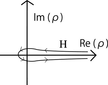
Figure 2: Integration contour to calculate Eq.(26).

3.2 Analytical results

Let us apply the argument of the previous section to DREM. For simplicity, we focus here on the case of the 1RSB transition at $n=n_{c}$ assuming $\alpha>1$ and $\beta>\beta_{c}$.

3.2.1 Locus of zeros

Eqs. (31) and (32) indicate that $\left(\partial^{2}/\partial n^{2}\right)\phi_{\rm RS2}(n)=(\alpha\beta^{2}/4)\left(1-\tanh^{2}(\beta_{c}/2)\right)>\left(\partial^{2}/\partial n^{2}\right)\phi_{\rm 1RSB}(n)=0$ at $n=n_{c}=\beta_{c}/\beta$, whereas $\left(\partial/\partial n\right)\phi_{\rm RS2}(n)=\left(\partial/\partial n\right)\phi_{\rm 1RSB}(n)=(\alpha\beta/2)\tanh(\beta_{c}/2)$ holds. This implies that the 1RSB transition is classified to the second order. The naive argument provided in the previous section means that the locus of zeros can be locally parameterized as

$$n\simeq n_{c}+v\exp\left(\pm(2l-1)\pi/4{\rm i}\right),$$ (33)

where $l=1,2$, $v\in\mathbb{R}$. However, this result must be corrected; the branch of $l=2$, which corresponds to the incident angle $3\pi/4$, never appears due to the following reason.

For $N\gg 1$, asymptotic evaluation of eq. (26) yields an expression

$$\left\langle Z^{n}\right\rangle \simeq N\alpha\beta e^{Nn\alpha\beta/2}$$ (34)

$$\times \int_{0}^{h_{2}^{-1}(1-\alpha^{-1})}dy\exp\left(N\left(-n\alpha\beta y+\left(1-\alpha+\alpha h_{2}(y)\right)\log 2\right)\right),$$ (35)

derivation of which is shown in [5]. Evaluating dominant contributions in the integral by the steepest descent method [16] indicates that the asymptotic expression is further simplified as

$$\left\langle Z^{n}\right\rangle\simeq\left\{\begin{array}[]{ll}p_{\rm RS2}e^{N\phi_{\rm RS2}(n)}+p_{\rm 1RSB}e^{N\phi_{\rm 1RSB}(n)},&n_{c}<{\rm Re}(n)<1,\cr p_{\rm 1RSB}e^{N\phi_{\rm 1RSB}(n)},&0<{\rm Re}(n)<n_{c},\end{array}\right.$$ (38)

depending on the position of $n$, where $p_{\rm RS2}=(\pi/(2N\alpha))^{1/2}(\cosh(n\beta/2))^{-1}$ and $p_{\rm 1RSB}=(N\alpha\beta(n_{c}-n))^{-1}$. This is because the absolute value of the integrand is maximized in the integral interval $0<y<h_{2}^{-1}(1-\alpha^{-1})$ for $n_{c}<{\rm Re}(n)<1$ while the right terminal point $y=h_{2}^{-1}(1-\alpha^{-1})$ offers a unique dominant contribution for $0<{\rm Re}(n)<n_{c}$. Equation (38) means that, for $N\gg 1$, there are no zeros of $0<{\rm Re}(n)<n_{c}$. Solving $\left\langle Z^{n}\right\rangle=0$ with respect to $n$ perturbatively in the vicinity of $n=n_{c}$ for $n_{c}<{\rm Re}(n)<1$ under a condition of $N\gg 1$ yields an asymptotic expression of the zeros

$$n_{k}\simeq n_{c}+\frac{4}{\beta}\left(1-\frac{1}{16k}\right)\cosh\left(\frac{\beta_{c}}{2}\right)\sqrt{\frac{k\pi}{N\alpha}}$$ (39)

$$\phantom{n\simeq n_{c}+}\times\exp\left(\pm\left(\frac{\pi}{4}+\frac{1}{8k\pi}\log(8k\pi^{2})\right){\rm i}\right)+o\left(N^{-1/2}\right),$$ (40)

$(k=1,2,\ldots)$, where $o\left(N^{-1/2}\right)$ represents contributions which are relatively negligible compared to $N^{-1/2}$.

This result indicates that the distance from the real axis to the closest zero, $n_{1}$, decays as $O(N^{-1/2})$ and, in the thermodynamic limit $N\to\infty$, the incident angle of the phase boundary converges to $\pi/4$. However, the angle between the real axis and the line connecting the transition point $n_{c}$ with the $k$th zero, $n_{k}$ $(k=1,2,\ldots)$, is larger than $\pi/4$ by $1/(8k\pi)\log(8k\pi^{2})$ independently of $N$ as long as $k$ is finite. This implies that for systems of finite sizes zeros in the vicinity of $n_{c}$ are expected to be placed in the left side of the phase boundary.

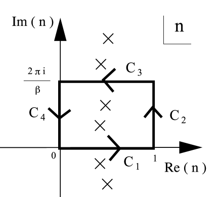
Figure 3: A cycle $\gamma$, the number of complex zeros inside which is evaluated utilizing the argument principle.

3.2.2 Number of zeros

Eqs. (31) and (32) can also be utilized to evaluate the asymptotic number of complex zeros. For this, let us consider a closed cycle $\gamma:C_{1}\to C_{2}\to C_{3}\to C_{4}$ as shown in figure 3. Application of the argument principle of the previous section to eqs. (31) and (32) yields the asymptotic number of zeros inside $\gamma$. $\gamma$ in figure 3 guarantees that the estimate does not vanish since the critical replica number $n_{c}=\beta_{c}/\beta$ is in the range $0<n<1$.

To simplify the analysis, we decompose the generating function as

$$\phi_{N}(n)=\frac{1}{N}\log\left<Z^{n}\right>=\Lambda(n)+{\rm i}\Omega(n)$$ (41)

where $\Lambda(n)$ and $\Omega(n)$ are real functions. The argument principle indicates that $N(2\pi)^{-1}\int_{\gamma}dn(\partial/\partial n)\Omega(n)$, which is proportional to the total variation of $\Omega(n)$ as $n$ goes around $\gamma$, accords with the number of zeros inside $\gamma$. For $N\gg 1$, we substitute $\phi(n)$ into $\phi_{N}(n)$, which makes it possible to analytically evaluate the variation.

Along $C_{1}$, both $\phi_{\rm RS2}(n)$ and $\phi_{\rm 1RSB}(n)$ lead to $\Omega(n)=0$. Therefore,

$$\Delta_{C_{1}}\Omega=\Omega(1)-\Omega(0)=0.$$ (42)

Along $C_{2}$, $\phi(n)=\phi_{\rm RS2}(n)=\log(2)+\alpha\log\left(\cosh\left(n\beta/2\right)\right)$ holds. This leads to

$$\Delta_{C_{2}}\Omega = {\rm Im}\left(\phi_{\rm RS2}\left(1+(2\pi/\beta){\rm i}\right)\right)-{\rm Im}\left(\phi_{\rm RS2}\left(1\right)\right)$$ (43)

$$= {\rm Im}\left(\alpha\log\left(-\cosh(\beta/2)\right)\right)=\alpha\pi,$$ (44)

where ${\rm Im}(z)$ denotes the imaginary part of a complex number $z$. Along $C_{3}$, $\phi(n)$ becomes real and therefore

$$\Delta_{C_{3}}\Omega=0.$$ (45)

Along $C_{4}$, on the other hand, $\phi(n)=\phi_{\rm 1RSB}(n)$ holds, which yields

$$\Delta_{C_{4}}\Omega = {\rm Im}\left(\phi_{\rm 1RSB}\left(0\right)\right)-{\rm Im}\left(\phi_{\rm 1RBS}\left((2\pi/\beta){\rm i}\right)\right)$$ (46)

$$= -{\rm Im}\left(\frac{\alpha\beta}{2}\tanh\left(\frac{\beta_{c}}{2}\right)\frac{2\pi{\rm i}}{\beta}\right)=-{\alpha\pi}\tanh\left(\frac{\beta_{c}}{2}\right).$$ (47)

These results indicate that the total number of zeros inside the cycle in the low temperature phase $\beta>\beta_{c}$ can be asymptotically estimated as

$$\nu_{est}\simeq\frac{N}{2\pi}\left(\Delta_{C_{1}}\Omega+\Delta_{C_{2}}\Omega+\Delta_{C_{3}}\Omega+\Delta_{C_{4}}\Omega\right)=\frac{\alpha N}{1+e^{\beta_{c}}}$$ (48)

for $N\gg 1$.

This indicates that the number of the zeros inside $\gamma$ grows proportionally to $N$. However, the total number of zeros over the complex plane of $n$ is infinite because $\left\langle Z^{n}\right\rangle$ is a transcendent function of $n$ and has period $2\pi/\beta$ in the imaginary direction. This is in contrast to the case of the Lee-Yang zeros with respect to $\beta$ for a typical sample of DREM [6, 7]. In this case, the partition function $Z(\beta)$ becomes a polynomial of $\beta$ and the number of zeros over the entire plane grows only linearly with respect to $N$, which yields a continuous distribution of zeros after being averaged over $\{\epsilon_{i}\}$.

3.3 Numerical results

In order to justify the analytically obtained results for $N\gg 1$, we numerically examined the zeros of $\left\langle Z^{n}\right\rangle=0$ for several $N$ utilizing the expression of eq. (26). Unfortunately, as eq. (26) is transcendent with respect to $n$, solving for the zeros algebraically is difficult. Therefore, we resorted to an iterative numerical method to search for the zeros.

We employed the secant method [17]. For solving an equation $f(z)=0$, this scheme iterates the recurrence relation

$$z_{t+1}=z_{t}-\frac{z_{t}-z_{t-1}}{f(z_{t})-f(z_{t-1})}f(z_{t}),$$ (49)

until $|z_{t}-z_{t-1}|$ becomes smaller than a feasible discrepancy level, which was here chosen to be $10^{-8}$. This update rule is somewhat similar to that of Newton’s method. Actually, the secant method can be regarded as an approximation of Newton’s method, which is obtained by replacing $(z_{t}-z_{t-1})/(f(z_{t})-f(z_{t-1}))$ with $f^{\prime}(z_{t})$ in eq. (49). A major advantage of this method is that there is no need to evaluate the first derivative. This property is useful when $f(z)$ is complicated, which is the case for the current objective system

To find all zeros inside $\gamma:C_{1}\to C_{2}\to C_{3}\to C_{4}$, we adopted the following strategy. We first covered the region inside $\gamma$ with a mesh of a fixed size in order to determine a set of initial values $n_{1}$ and $n_{2}$, which are required when utilizing the secant method. Two adjacent points in the vertical direction on the mesh were taken as the initial points. In the iteration of eq. (49), a calculated new point may step out of the region. In such cases, we changed the pair and tried the search again. Once we found a root $a_{1}$, we replaced $\left\langle Z^{n}\right\rangle$ with $\left\langle Z^{n}\right\rangle/(n-a_{1})$ and continued the calculation. After trying every pair of initial values, we reduced the mesh size and searched for the roots again. We finished these procedures when we were unable to find a new root.

Table 1 shows dependence of the number of zeros on the system size $N$. This indicates that the number of zeros obtained numerically is reasonably consistent with the number obtained from analytical evaluation (48), implying that the number of the search trials has been sufficiently many.

$N$	$\nu_{est}$	$\nu$
5	4.3	5
10	8.6	10
15	12.9	14
20	17.1	19
25	21.4	23

Table 1: The number of complex zeros with respect to $n$ in the cycle shown in figure 3 for $\alpha=4$ and $\beta=3\beta_{c}$. The estimated number is calculated from eq. (48) and the actual number $\nu$ is evaluated by numerically searching for the zeros using eq. (49).

Figure 4 shows results of the search for $N=5,10,15,20$ and $25$. The curve represents the locus of the zeros in the limit as $N\to\infty$, which was evaluated using the condition ${\rm Re}(\phi_{\rm RS2}(n))={\rm Re}(\phi_{\rm 1RSB}(n))$. As we expected, the incident angle of the locus to the real axis was $\pi/4$, indicating that the first discontinuity of $\phi(n)$ appears at the level of the second derivative.

The markers represent data obtained from the numerical search. These show that the zeros approach the locus from the left side as $N$ becomes larger, as we expected. Makers of figure 5 stand for zeros obtained from the asymptotic expression of eq. (38). These exhibit behavior qualitatively similar to that of the exact expression; but deviation is not negligible, which is presumably due to finite size effects. Nevertheless, the distance of $n_{1}$ to the real axis (${\rm Im}(n_{1})$) shows a fairly good consistency with the theoretical prediction of eq. (40), validating our asymptotic analysis based on the steepest descent method (figure 6).

In conclusion, the overall consistency between the analytical and numerical evaluations justifies the current analysis based on eq. (26).

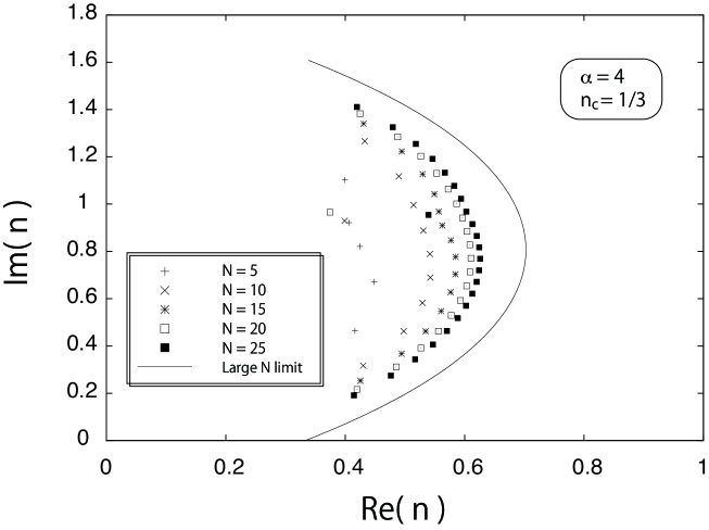
Figure 4: Complex zeros of the moment of the partition function of DREM for $\alpha=4$ and $\beta=3\beta_{c}$. The transition point in this case is determined to be $n_{c}=\beta_{c}/\beta=1/3$. The curve represents the locus of zeros in the thermodynamic limit, which is evaluated using ${\rm Re}(\phi_{\rm RS2}(n))={\rm Re}(\phi_{\rm 1RSB}(n))$. The incident angle of the curve to the real axis is $\pi/4$, which indicates that the transition of $\phi(n)$ is analogous to a phase transition of the second order. Numerical data (markers) approach the locus as the system size $N$ increases from $N=5$ to $25$ in steps of $5$.

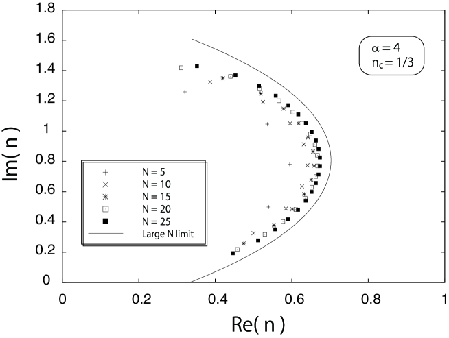
Figure 5: Complex zeros obtained from the asymptotic expression of eq. (38) for $\alpha=4$, $\beta=3\beta_{c}$ and $N=5,10,\ldots,25$.

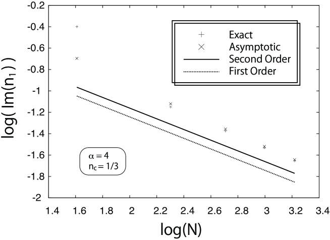
Figure 6: Distance of $n_{1}$ to the real axis (${\rm Im}(n_{1})$) versus system size $N$. Markers, $+$ and $\times$, represent the results for the exact expression of eq. (26) and for the asymptotic one of eq. (38), respectively. The full line shows theoretical prediction ${\rm Im}(n_{1})=5\sqrt{\pi}/(4\beta\sqrt{N\alpha})\cosh(\beta_{c}/2)\sin(\pi/4+(1/8)\log(8\pi^{2}))$, which is obtained by neglecting the $o(N^{-1/2})$ contribution in eq. (40), while the correction $(1/8)\log(8\pi^{2})$ is omitted in the broken line. These support our theoretical predictions which indicate that the distance vanishes as $O(N^{-1/2})$ and positive corrections of the incident angle from $\pi/4$ exist for $n_{k}$ independently of $N$ as long as $k=1,2,\ldots$ is finite.

4 Summary

In summary, we have characterized analyticity breaking with respect to the replica number $n$ which arises in the discrete random energy model (DREM) by examining zeros of the moment of the partition function over the complex $n$ plane. To do this, we utilized an exact expression of the moment of the partition function, which was introduced by the authors in a related paper [5]. The expression is valid for $\forall{n}\in\mathbb{C}$ and useful for numerically evaluating the moment of finite size systems. Taking the thermodynamic limit of the expression at sufficiently low temperatures indicates that analyticity breaking occurs at a critical replica number $0<n_{c}<1$, which can be regarded as the origin of the one step RSB (1RSB) solution. Perturbatively evaluating the zeros in the vicinity of $n_{c}$ based on the expression utilizing the steepest descent method shows that the distance from the real axis to the closest zero decays as $O(N^{-1/2})$ when the system size $N$ is large. Examining the asymptotic form of the locus of the zeros in the thermodynamic limit $N\to\infty$ implies that the transition is analogous to a phase transition of the second order. We also evaluated the asymptotic number of zeros inside a unit cycle shown in figure 3 based on the expression. Zeros numerically obtained for finite size systems are reasonably consistent with the analytical predictions.

The approach developed here is also applicable to the standard continuous random energy model [18], and this approach yields results qualitatively the same as those for DREM. This implies that the 1RSB transitions observed in a family of REMs can be generally characterized by the complex zeros in a similar manner.

A natural question to ask is whether another type of RSB, full RSB (FRSB), can be characterized similarly by the complex zeros. Recently, one of the authors examined the zeros of tree systems in a vanishing temperature limit [19]. Although some of the systems are conjectured to exhibit FRSB at a certain critical number, numerical data about the zeros seem irrelevant to the FRSB transition. It is, therefore, desirable to explore other systems in order to assess whether or not the irrelevance of the zeros to FRSB is specific to tree systems.

References

References

- [1] Dotzenko V S 2001 Introduction to the Replica Theory of Disordered Statistical Systems (Cambridge: Cambridge University Press)
- [2] van Hemmen J L and Palmer R G 1979 J. Phys. A: Math. Gen.12 563
- [3] Sherrington D and Kirkpatrick S 1975 Phys. Rev. Lett. 35 1972
- [4] Ogure K and Kabashima Y 2004 Prog. Theor. Phys 111 661
- [5] Ogure K and Kabashima Y 2009 J. Stat. Mech. P03010
- [6] Moukarzel C and Parga N 1991 Physica A177 24
- [7] Moukarzel C and Parga N 1992 Physica A185 305
- [8] Yang C N and Lee T D 1952 Phys. Rev.87 404
- [9] Lee T D and Yang C D 1952 Phys. Rev.87 410
- [10] Grossmann S and Rosenhauer W 1969 Z. Physik 218 437
- [11] Grossmann S and Lehmann V 1969 Z. Physik 218 449
- [12] Ahlfors L V 1953 Complex Analysis (New York: McGraw-Hill)
- [13] Marinari E 1984 Nucl. Phys. B 235 123
- [14] Janke W, Johnston D A and Kenna R 2006 Nucl. Phys. B 736 319
- [15] Titchmarsh E C 1932 The Theory of Functions (Oxford: Oxfprd University Press)
- [16] Keener J P 1988 Principles of Applied Mathematics: Transformation and Approximation (Redwood City: Addison-Wesley)
- [17] Press W H, Flannery B P, Teukolsky S A and Vetterling W T 1992 Numerical Recipes in FORTRAN: The Art of Scientific Computing, 2nd ed. (Cambridge: Cambridge University Press)
- [18] Derrida B 1981 Phys. Rev.B 24 2613
- [19] Obuchi T, Kabashima Y and Nishimori H 2009 J. Phys. A: Math. Theor. 42 075004(27pp)