Effects of disorder on lattice Ginzburg-Landau model of
$d$-wave superconductors and superfluids

Abstract

We study the effects of quenched disorder on the two-dimensional $d$-wave superconductors (SC’s) at zero temperature by Monte-Carlo simulations. The model is defined on the three-dimesional (3D) lattice and the SC pair field is put on each spatial link as motivated in the resonating-valence-bond theory of the high-$T_{\rm c}$ SC’s. For the nonrandom case, the model exhibits a second-order phase transition to a SC state as density of charge carriers is increased. It belongs to the universality class different from that of the 3D XY model. Quenched disorders (impurities) are introduced both in the hopping amplitude and the plaquette term of pair fields. Then the second-order transition disappears at a critical concentration of quenched disorder, $p_{c}\simeq 15\%$. Implication of the results to cold atomic systems in optical lattices is also discussed.

Effects of disorder on phase structures and phase transitions have been studied for various systems. In particular, the high-$T_{\rm c}$ materials are microscopically highly nonuniform and it is suggested that there exists a spinglass like phase near the phase transition point of superconductivity (SC) at low temperatures ($T$)SG . Furthermore, existence of a Bose glass was recently suggested in the Mott-insulating phase of cold atomic systems in random potentialsBoseglass . In the present paper, being motivated in part by these observations, we shall study effects of quenched disorders on SC’s by using a lattice Ginzburg-Landau (GL) model of unconventional $d$-wave SC’s. The model in its pure case was introduced as the GL theory of the resonating-valence-bond (RVB) field for the t-J modelnm , and the case of including interaction with the electromagnetic (EM) field has been investigated recentlysmi . We expect that this model also describes superfluid phase of fermionic atoms in cold atomic systems in optical lattices. There, the effects of disorders can be investigated well under control.

We are interested in quantum SC phase transition of the two-dimensional (2D) model at $T=0$. The model in path-integral representation is described in terms of the following RVB-type Cooper pair field $U_{xj}$:

$$U_{xj}\sim\langle\psi_{x+j,\uparrow}\psi_{x\downarrow}-\psi_{x+j,\downarrow}\psi_{x\uparrow}\rangle,$$ (1)

where $x(x_{0},x_{1},x_{2})$ is the site of the 3D cubic lattice of size $V=L^{3}$ with periodic boundary condition and $j=1,2$ denotes the spatial direction and also the unit vector in $j$-th direction. $\psi_{x\sigma}$ is the electron annihilation operator at site $x$ and spin $\sigma=\uparrow,\;\downarrow$. In the $d_{x^{2}-y^{2}}$-wave SC, the Cooper pair amplitudes in $x=x_{1}$ and $y=x_{2}$ have the opposite signatures as $\langle U_{x1}U^{\dagger}_{x2}\rangle<0$.

Below we shall neglect the effects of the EM field and focus on the effects of quenched disorders. The action of the clean system is then given as follows:

$$A = g\sum_{x}\Big{[}c_{2}\>\bar{U}_{x2}U_{x+2,1}\bar{U}_{x+1,2}U_{x1}$$

$$+c_{3}\>(\bar{U}_{x+1,2}U_{x1}+U_{x+2,1}\bar{U}_{x+1,2}$$

$$\ \ \ \ +\bar{U}_{x2}U_{x+2,1}+U_{x1}\bar{U}_{x2})$$

$$+c_{4}\>(\bar{U}_{x+2,1}U_{x1}+\bar{U}_{x+1,2}U_{x2})$$

$$+c_{5}\>(\bar{U}_{x+0,1}U_{x1}+\bar{U}_{x+0,2}U_{x2})+\mbox{c.c.}\Big{]},$$ (2)

where we consider the London limit and set $U_{xj}$ a U(1) variable, $U_{xj}=\exp(i\theta_{xj}),\ \theta_{xj}\in[-\pi,\pi)$. The overall factor $g$ plays a role of $1/\hbar$ and controls quantum fluctuations. When we fix $c_{i}$, $g$ can be taken as an increasing function of the carrier concentration $\delta$. (In the t-J model $\delta$ is the hole density.) The $c_{2}$ terms controls fluctuation of flux of $U_{xj}$’s around each spatial plaquette. The $c_{3}$ and $c_{4}$ terms represent the spatial hopping of $U_{xj}$, whereas the $c_{5}$ term describes the hopping in the imaginary-time ($0$-th) direction. The partition function $Z$ is given by $Z=\int[dU]\exp(A),\ [dU]=\prod_{x,j}d\theta_{xj}/(2\pi)$. We consider the parameter region $c_{3}<0$ to expect $\langle U_{x1}U^{\dagger}_{x2}\rangle<0$, although $Z(c_{3})=Z(-c_{3})$ because of the change of variables $U_{x1}\rightarrow-U_{x1}$. The action $A$ is related to the action $A_{\rm Higgs}$ of the U(1) Higgs gauge theory that is obtained from Eq.(2) by the replacement $U_{xj}\rightarrow\bar{\phi}_{x+j}U_{xj}\phi_{x}$, where $\phi_{x}=\exp(i\varphi_{x})$ is the U(1) Higgs field. $A_{\rm Higgs}$ is invariant under time-independent local gauge transformation $\varphi_{x}\rightarrow\varphi_{x}+\lambda_{x},\ \theta_{xj}\rightarrow\theta_{xj}+\lambda_{x+j}-\lambda_{x}$ where $\lambda_{x(x_{1},x_{2})}$ is an $x_{0}$-independent function. Actually, $A$ is viewed as the gauge-fixed version of $A_{\rm Higgs}$ in the unitary gauge $\phi_{x}=1$.

Queched disorder is introduced in the system (2) by replacing the coefficinets $c_{2,3,4}$ as spatial-plaquette dependent ones. First, we consider the 2D spatial plane with fixed $x_{0}$, say $x_{0}=0$. Among $L^{2}$ plaquettes in the plane we choose $p\times L^{2}$ plaquettes randomly as ones at which impurities reside. We call it a sample. We consider that the configuration of “wrong” plaquettes is $x_{0}$-independent because the location of impurities are fixed along the imaginary time. Then we reverse the values of $c_{2,3,4}$ for interaction terms contained in these plaquettesdisorder . Thus the new plaquette-dependent coefficients $c^{p}_{2,3,4}$ are given by

$$c^{p}_{2,3,4}=\left\{\begin{array}[]{cl}c_{2,3,4}&\mbox{with\ probability $1-p$}\\ -c_{2,3,4}&\mbox{with\ probability $p$},\end{array}\right.$$ (3)

for each spatial plaquette. Please note $c^{p}_{5}=c_{5}$. Then the partition function $Z_{p}$ and the free energy $F_{p}$ per site of one sample are given by

$$Z_{p}=\int[dU]\exp(A_{p})=\exp(-VF_{p}),$$ (4)

where $A_{p}$ is obtained from Eq.(2) by replacing $c_{i}$ by $c^{p}_{i}$. To obtain an ensemble average $\langle O\rangle$ of an observable $O(\{U_{xj}\})$ in the disordered system, we first prepare $N_{s}$ samples and calculate the quantum-mechanical average $\langle O\rangle_{s}$ for the $s$-th sample ($s=1,\cdots,N_{s})$. Then we average it over samples,

$$\langle O\rangle=\frac{1}{N_{s}}\sum_{s=1}^{N_{s}}\langle O\rangle_{s},\langle O\rangle_{s}=Z_{p_{s}}^{-1}\int[dU]O\exp(A_{p_{s}}).$$ (5)

For the MC simulations, we used the standard Metropolis algorithmma . The typical statistics used was $10^{5}$ sweeps per block and the average and MC errors were estimated over 10 blocks for each sample. Then we take quenched averages over $N_{s}=30\sim 50$ samples. We estimated standard deviation of physical quantities like “specific heat” over samples (we call it sample error) as a function of $N_{s}$, which becomes stable for $N_{s}\stackrel{{\scriptstyle>}}{{\sim}}30$.

Figure 1: Specific heat $C$ for $p=0$ as a function of $g$ with $c_{2}=-c_{3}=c_{4}=c_{5}=1$. Error bars represent MC errors. System-size dependence of its peak supports existence of a second-order phase transition.

Figure 2: Correlation function $G(r)$ for various values of $g$ with $c_{2,4,5}=-c_{3}=1$. Critical coupling $g_{c}$ is estimated $g_{c}=0.154$ for $L=20$. Data show that for $g>g_{c}$ there exists SC LRO, whereas $g<g_{c}$ no LRO.

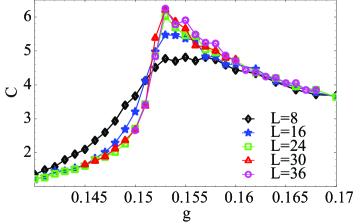
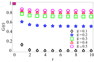
Let us first consider the nonrandom case, $p=0$. We studied the phase structure by calculating the “internal energy” per site $E=-\langle A\rangle/V$ and the “specific heat” per site $C=\langle(A-\langle A\rangle)^{2}\rangle/V$. Typical behavior of $C$ is shown in Fig.1, which indicates a second-order phase transition at $g=g_{c}\simeq 0.154$. This transition has been predicted in Ref.nm and also observed in the presence of the EM gauge interactionssmi . In order to verify that it is a transition to a SC phase, we measured the correlation function of $U_{xj}$, the order parameter field of SC,

$$G(r)={1\over 4V}\sum_{x,i\neq j}\langle\bar{U}_{xj}U_{x+ri,j}\rangle+\mbox{c.c.}$$ (6)

We present $G(r)$ in Fig.2. It is obvious that there exists SC long-range order (LRO) for $g>g_{c}$, whereas no LRO for $g<g_{c}$lro . Therefore the observed transition is nothing but the SC phase transition.

The critical exponents for $c_{2,4,5}=-c_{3}=1$ were estimated by the finite-size scaling analysis for $C$. We obtained $\nu=1.5,\;\alpha=0.285$ and the critical coupling $g_{\infty}=0.153$. When $c_{2}=c_{3}=0$, the system (2) reduces to a set of decoupled 2D XY spin models [$U_{xj}$ plays the role of an XY spin], each of which has the Kosterlitz-Thouless transition. The $c_{2}$ and $c_{3}$ terms couple these 2D XY spins. From the above values of critical exponents, we judge that the present phase transition does not belong to the universality class of the 3D XY model having $\nu=0.6721(13)$exponent .

Let us next turn to the random case, $p>0$. At first, we consider the $gc_{2}-gc^{\prime}$ plane where $c^{\prime}\equiv-c_{3}=c_{4}=c_{5}$, and search for the location of the peak of $C$. In Fig.3, we present the peak location of $C$ for given disorder concentration $p=0.0,0.10,0.20.$ For $p=0.0$, the peak line expresses the second-order transition as we saw in Figs.1 and 2. We see that the region of the normal (non SC) state increases as $p$ increases, although we need to check whether the location of this peak expresses genuine SC transition for $p>0$. Below we examine it

Figure 3: Location of the peak of $C$ with $L=12$ and $N_{s}=30$ in the $gc_{2}-g\times(-c_{3}=c_{4}=c_{5})$ plane for $p=0,0.10,0.20$. The region of disorder “phase” increases as $p$ increases.

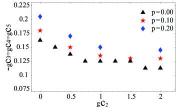
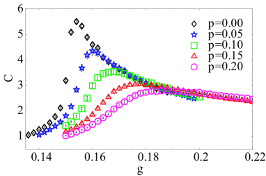
by focusing on the specific case $c_{2}=-c_{3}=c_{4}=c_{5}=1$ with the varying parameter $g$ and calculate $E,\ C,\ G(r)$, etc. Density of quenched disorder that we studied is $p=0.05,0.10,0.15$ and $0.20$.

We first present the result of $C$ in Fig.4. The signal of the second-oder phase transition at $p=0$ is getting weaker as $p$ is increased, and also the location of the peak moves to larger $g$.

Figure 4: Specific heat $C$ for $L=16$ with $N_{s}=30$ vs $g$ for $p=0.0,\cdots,0.20$. Error bars here and below represent sample errors. The peak around the SC phase transition is getting weaker as $p$ is increased. Location of the peak moves to larger $g$.

Figure 5: The system size dependence of $C$ with $N_{s}=30$ for $p=0.10,\ 0.15,\ 0.20$. $C$ for $p=0.10$ shows SSD, which supports a second-order phase transition to SC state. $C$ for $p=0.15$ has less SSD, and $C$ for $p=0.20$ shows no SSD for $L=16,24$.

Figure 6: $D(g)\equiv gdC(g)/dg$ with $N_{s}=30$ vs $g$ for various $L$. (a)$p=0.10$; (b)$p=0.15$; (c)$p=0.20$. The cases (a) and (b) show SSD, while the case (c) shows almost no SSD.

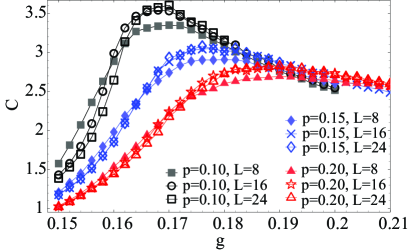
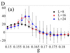
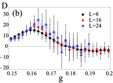
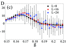
Next, in Fig.5, we present the system-size dependence (SSD) of $C$ for $p=0.10,\ 0.15$ and $0.20$. We also calculated the derivative of $C$, $D(g)\equiv gdC(g)/dg$, to identify the order of the phase transition. Results are shown in Fig.6. From these results, we judge that there exists a second-order transition for $p\leq 0.10$ whereas it changes to a crossover for $p\geq 0.20$. The case of $p=0.15$ seems to have no SSD in $C$ but have certain SSD for $D(g)$. Therefore, the transition in the $p=0.15$ case might be of third order.

Figure 7: SC correlation function $G(r)$ for $L=20$ with $N_{s}=50$. (a)$p=0.10$; (b)$p=0.15$; (c)$p=0.20$. (d) $G(r=10)$ for (a,b,c) vs g. SC “transition point” $g_{c}$ is estimated from the specific heat $C$ as $g_{c}\simeq(a)0.168,\ (b)0.17,\ (c)0.18$. Fig.(d) supports that LRO developes for $g>g_{c}$ in (a).

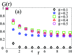
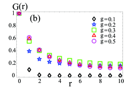
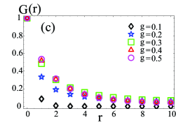
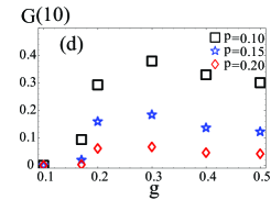
To study if the SC state persists even for $p\geq 0.20$, we measured the SC correlation $G(r)$ averaged over samples with randomly generated $c^{p}_{i}$. In Fig.7 we present the results for $p=0.10,\ 0.15$ and $0.20$. It supports that for $p=0.10$ there exists the SC LRO for $g>g_{c}$ whereas for $p=0.20$ no LRO for any values of $g$. This observation leads to the conclusion that the SC phase disappears for $p\geq 0.20$, i.e., there is a multicritical point $p_{\rm mc}$ near $p=0.15$ in the $g-p$ phase diagram.

Figure 8: Phase diagram in the $p-g^{-1}$ phase diagram for the lattice model of dirty $d$-wave SC with $c_{2}=-c_{3}=c_{4}=c_{5}=1$. Possible Bose glass phase is suggested. There should be a multicritical point near the line $p=0.15$.

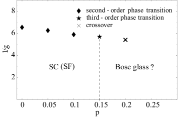
It is interesing to ask what kind of phase is realized in the region $p>p_{\rm mc}$ and $g>g_{\rm cr}$, where $g_{\rm cr}$ is the crossover coupling determined by the peak location of the specific heat. Probably, in the case of the doped AF magnets with strong inhomogeneity, this phase may simply correspond to dirty “normal” metallic state. We think that the present model given by Eq.(2) also describes the superfluid $d$-wave RVB state of fermionic atoms in 2D optical lattice, which was recently proposed by sereval authorsdwave . Random disorders can be introduced into the systems by a laser speckle or by an incommensurate bichromatic potentail. In that experimental setup, there is an interesting possibility that a Bose glass phase, which is an analogue of the spin glass phase, is realized there. For ultracold strongly interacting ⁸⁷Rb bosons, a Bose glass phase is suggested by experimentsBoseglass . In the experiments of cold atom systems in optical lattices, the Bose glass phase has no long-range coherence but excitations are gapless. In Fig.8, an expected phase diagram of the present lattice model of dirty $d$-wave SC and superfluidity (SF) is shown. We think that existence of the Bose glass phase is examined theoretically by the standard analytical and numerical methods applied for spin glasssg ; z2 .

References

- (1) F.C. Chou, N.R. Belk, M.A. Kastner, R.J. Birgeneau, and A. Aharony, Phy. Rev. Lett. 75, 2204(1995).
- (2) L. Fallani, J.E. Lye, V. Guarrera, C. Fort, and M. Inguscio, Phys. Rev. Lett. 98, 130404(2007).
- (3) G. Baskaran and P. W. Anderson, Phys. Rev. B37, 580(1988); A. Nakamura and T. Matsui, Phys. Rev. B37, 7940(1988); Y. Munehisa and T. Matsui, Phys. Rev. B43, 11388(1991).
-
(4)
K. Sawamura, Y. Moribe, and I. Ichinose,
Nucl. Phys.
B785, 307(2007); K. Sawamura, I. Ichinose, and
Y. Moribe, Mod. Phys. Lett. A23, 2821(2008); See also Ref.UV . - (5) T. Ono, Y. Moribe, S. Takashima, I. Ichinose, T. Matsui, and K. Sakakibara, Nucl. Phys.B 764, 168(2007).
- (6) One wrong plaquette gives rise to four terms, two terms, and one term (except for their c.c.) with the sign-reversed coefficients.
- (7) N. Metropolis, A. W. Rosenbluth, M. N. Rosenbluth, A. M. Teller, E. Teller, J. Chem. Phys. 21, 1087(1953).
- (8) Because we deal with the gauge fixed version of expectation values of gauge-noninvariant quantities like may be nonvanishing without conflicting Elitzur’s theorem.
- (9) H. G. Ballesteros, L. A. Fernández, V. Martin-Mayor, A. Munoz Sudupe, Phys. Lett. B387, 125(1996).
- (10) W. Hofstetter, J. I. Cirac, P. Zoller, E. Demler, and M. D. Lukin, Phys. Rev. Lett.89, 220407(2002); S. Trebst, U. Schollwöck, M. Troyer, and P. Zoller, Phys. Rev. Lett.96, 250402(2006).
- (11) S. F. Edwards and P. W. Anderson, J. Phys. F5, 965(1975); D. Sherrington and S. Kirkpatrick, Phys. Rev. Lett. 35, 1792(1975); M. Mezard, G. Parisi, and M.A. Virasoro, “Spin Glass Theory and Beyond”, World Scientific(1987).
- (12) It is interesting that the study of 3D Ising model with random couplings by M. Hasenbusch, F. P. Toldin, A. Pelissetto, E. Vicari, arXiv:0810.0685, also shows the similar phase diagram as Fig.8 with a glass phase. L. Dang, M. Boninsegni, and L. Polletar, arXiv:0812.3417, also discuss the disorder-induced glassy SF state.