Universality in the Vibrational Spectra of Amorphous Systems
A thesis submitted in partial fulfillment
of the requirements
for the degree of
Doctor of Philosophy.
Gurpreet Singh Matharoo
![[Uncaptioned image]](/html/0812.4613/assets/x1.png)
School of Physical Sciences
Jawaharlal Nehru University
New Delhi - 110 067
September 2005
Dedication…
This thesis is dedicated to the memory of
my beloved father
Mr. Shivcharan Singh Matharoo.
DECLARATION
I hereby declare that the work reported in this thesis is entirely original and has been carried out by me in the School of Physical Sciences, Jawaharlal Nehru University, New Delhi. The work has been supervised by Dr. Subir Kumar Sarkar. I further declare that it has not formed the basis for the award of any degree, diploma, associateship or similar title of any university or institution.
September, 2005 Gurpreet Singh Matharoo
Prof. H. B. Bohidar Dr. Subir Kumar Sarkar
Dean Thesis Supervisor
School of Physical Sciences School of Physical Sciences
Jawaharlal Nehru University Jawaharlal Nehru University
New Delhi - 110067 New Delhi - 110067
Acknowledgements
It would not have been possible for me without my advisor Dr. Subir Kumar Sarkar to complete this thesis. He not only taught me Physics and the art of computer programming but also to do things sincerely and in a truthful manner. I still have a very long way to go and I do hope that he supports me in the same manner in the years to come.
I had the privilege to work with Prof. Akhilesh Pandey in the first part of the thesis. He not only helped me with theoretical ideas but also corrected me at many places in my computer programs.
I would like to thank Prof. Shankar P. Das for his concern and valuable suggestions and discussions from time to time. I have benefitted from them on many occasions.
Prof. Sanjay Puri has been a combination of teacher and a senior friend to me. I have not only benefited from him in Statistical Mechanics but also as a player on the cricket field.
My teachers at Delhi University, namely, Prof. S. K.Muthu, Prof. K. L. Baluja and Dr. A. K. Kavathekar have been a constant source of encouragement to me for almost seven years now.
In SPS, I have spent a lot of quality time with Vikas, Anjana, Charan, Madhusudan Niladri, Navendu, and Ruchi. They have helped me a lot in tackling various problems.
Manju Chattopadhyay, Ashish Tyagi, Sanjeev Kumar and Bhavna Vidhani are some very important names in my life. I would like to thank all the friends who have written about me in my autograph book, their comments will remain as a treasure with me all the time.
I would also like to thank my mother for everything.
The acknowledgment will be incomplete if I dont mention the name of my best friend Robin. Finally, thanks Vinayak! for being there with me all the time.
List Of Publications
-
1.
Universality in the Vibrational Spectra of Single-Component Amorphous Clusters.
Subir K. Sarkar, Gurpreet S. Matharoo and Akhilesh Pandey,
PHYSICAL REVIEW LETTER 92, 215503 (2004). -
2.
Vibrational Spectra of Amorphous Clusters : Universal Aspects.
Gurpreet S. Matharoo, Subir K. Sarkar and Akhilesh Pandey,
PHYSICAL REVIEW B 72, 075401 (2005). -
3.
Vibrational Spectra of Simple Single-Component Systems: Evolution with Disorder and Passage to Quasi-Universality.
Subir K. Sarkar and Gurpreet S. Matharoo.
(to be submitted).Note: Chapters 2 to 4 of this thesis are based primarily on the papers 1 and 2 listed above. Chapter 5 is based on the preprint listed as paper 3.
-
Bibliography . . . . . . . . . . . . . . . . . . . . . . . . . . . . . . . . .
Chapter 1 Introduction
The concept of universality has been familiar in physics for several decades now [1] and has received widespread usage in many areas. In this thesis we examine the applicability of this concept to the domain of amorphous systems [2-22]. In particular we examine the theme of universality in the context of the vibrational spectra of such systems. We consider both clusters and bulk systems. Amorphosity immediately introduces some severe complications that have been the subject of a lot of attention for many years now [23-65]. Thus, even within the harmonic approximation, which we use consistently everywhere in this thesis, computation of the vibrational spectrum poses serious difficulties in any analytical scheme and invariably various kinds of approximations are used. These approximations may be with respect to both the equilibrium structure of the disordered system and the actual computation of the normal modes around this structure. Our computation, which is entirely numerical in nature, however makes no assumptions beyond the nature of the potential that describes the interaction amongst the constituent particles of the system. This is due to the fact that any candidate configuration for a solid state structure, amorphous or crystalline, must correspond to a local minimum of the potential energy function which can be computed very accurately using standard numerical techniques. These minima are also called ‘inherent structures’. For amorphous states the positional arrangement of the constituent units is highly disordered. The vibrational spectrum corresponding to a particular stable configuration is derived from the solutions of an eigenvalue problem in which the Hessian matrix for that configuration is involved. When the configuration is disordered, it is clear that the corresponding Hessian matrix will have substantial amount of randomness in it. Thus, it is not surprising that ideas from the theory of Random Matrices have been used in recent times to examine the vibrational spectra of disordered systems [32-34,55,61,66-68]. Infact, this is a key element in our analysis of the universal aspects of the vibrational spectra of disordered systems. Random Matrix theories have been used extensively [69-78] for the analysis of statistical fluctuations of the spectra of complex quantum systems such as complex nuclei, atoms, molecules, quantum chaotic systems, disordered mesoscopic systems etc. Study of the spectra of these systems has revealed that although the smooth part of the density of states will be system dependent, the fluctuations around the mean densities are universal and there are only three universality classes. In contrast, we look for universality both in the spectral fluctuations and in the density of states.
We have studied both clusters and bulk systems while investigating amorphous states. We have varied the nature of interaction amongst the particles of the system under consideration in order to reveal the possible presence of universality (i.e. independence of the potential). For clusters, the number of particles is varied to investigate the effect of finite size on various properties. To study bulk amorphous systems, we actually use periodic crystals with as large a primitive cell as possible. For any finite disorder, the number of particles in the primitive cell should ideally be made arbitrarily large. However, in practice, this is limited by the available computational resources. We should note here that due to the periodic nature of our approximation to the bulk disordered system, the analysis of spectral fluctuations becomes a lot more subtle and has not been reported in this thesis. We report results only on: (1) Universality in the density of states for clusters, (2) Universality in spectral fluctuations in the case of clusters, and (3) Universality in the density of states for bulk amorphous systems. In the following two paragraphs, we provide a summary of the results reported in the subsequent chapters.
Chapter 2 describes the study of universality in both density of states and statistical fluctuations in clusters made up of only one type of particle. We have used four different kinds of potentials. Of these, two belong to the ‘sum over pairs’ category and the other two contain many body interactions and hence are suitable for metals. The two primary results are: (1) The spectral fluctuations are described by the Gaussian Orthogonal Ensemble of random matrices to an extraordinarily high degree of accuracy and (2) Over a large central region of the vibrational spectrum, the density of states is described by the same functional form, containing one scale of frequency, in all cases. In chapter 3 we extend the studies of chapter 2 to binary systems in order to see how general are the results obtained for single component systems. We find that, atleast for the limited class of binary systems that we have studied, results for single component systems are reproduced. Thus, additional complexity does not cause any essential change in the results. In chapter 4 we examine the question of possible universality of the density of states over the entire spectrum rather than over only a limited central part of it. From our analysis of the data, it seems that universality of the form of the density of states does not extend over the entire spectrum for the potentials and system sizes investigated as far as clusters are concerned. This question is again taken up, for bulk systems, in the next chapter.
In chapter 5 we show that there are indeed certain limiting situations in which the normalized density of states assume a universal shape over the entire spectrum. Here we study systems made up of point particles that interact via two body forces only. The generic shape of this two body potential has a minimum at a certain distance at which the potential is negative. For larger distances the potential rapidly rises zero. At shorter distances also the potential rapidly rises either to a finite value or to an infinite value. The critical parameter for our purposes is how fast the curvature of this potential changes around the minimum. We introduce a parameter that quantifies the rapidity of this variation and we find that when this parameter becomes very large, the vibrational spectrum for completely disordered states assumes a shape that does not depend on the specific functional form of the potential that is tuned to achieve the very fast variation of the curvature around the minimum. We study the implications of these observations in understanding the quasi-universal shape that has been observed recently for the vibrational spectra of molecular glasses [65]. The methodology that is used for the investigation of the bulk amorphous systems has also been used in this chapter to study how the nature of the vibrational spectrum changes as one goes from crystalline state to completely amorphous states. For example, this gives a detailed picture of how excess vibrational modes develop in both the low frequency and high frequency domains of the spectrum. The accumulation in the low frequency domain is the reason behind the existence of what are called ‘boson peaks’[21-22, 45-65]. Although there are model theoretical calculations that study the evolution of the vibrational spectrum with increasing disorder, our calculation is distinguished by the fact that we do not need to use any specific model of disorder. Once the choice of potential is made, there is no need to make any further approximation.
Chapter 2 Universality of Statistical Fluctuations : Single-Component Amorphous Clusters
In this chapter we explore the theme of universality in the vibrational spectra of amorphous clusters made up of only one kind of constituent units (atoms or molecules) [67-68]. All our clusters are three dimensional and to check for universality, we use different kinds of potentials available in the literature [79-82]. More specifically, they are Lennard-Jones, Morse, Sutton - Chen and Gupta potentials. The explicit expressions of these four types are given by
Lennard-Jones potential:
| (2.1) |
with the factor of 4 omitted while calculating vibrational frequencies.
Morse potential:
| (2.2) |
with the value of .
Sutton - Chen potential:
| (2.3) |
We take the value of to be equal to 39.432 which corresponds to nickel.
Gupta potential:
| (2.4) |
The values of A, p and q are material specific and we have used the values applicable to nickel or vanadium.
In all the expressions given above is the distance between the particles labelled i and j. N is the total number of particles in the cluster. As far as the functional forms are concerned, Lennard-Jones and Morse are of the type ‘sum over pairs’ whereas the Sutton - Chen and Gupta potentials, which are often used to describe metallic clusters, contain many body interactions in them. Choice of these two distinct families of potentials is deliberate since universality is a primary theme here and we want to explore as many qualitatively distinct kinds of potentials as possible.
In order to compute the vibrational spectra of amorphous clusters the first step that needs to be taken is the generation of the stable geometries around which vibration takes place. Obviously, any such geometry will correspond to a local minimum of the potential energy function in the configuration space. Configurations corresponding to these minima are also called “inherent structures”. Each such inherent structure is a candidate for the geometry of a (atleast) metastable cluster at sufficiently low temperature. There are many methods available to generate these inherent structures. The method we have used is called “Homotopy Minimization” [83]. In this method if we need to generate a local minimum of a function , we actually perform minimization of a sequence of functions of the form . Here is an appropriately selected simple function. is a parameter that changes its values from 0 to 1 in a finite number of steps (about 20). In the first step of the homotopy minimization the initial guess of the configuration is a random distribution of the elements of the cluster within a sphere of suitable radius. If the radius is too large, the process of minimization is very slow and if it is too small, it may cause numerical instability due to high gradients that may be generated. As the value of keeps changing subsequently, the initial guess at any stage for the configuration is the one that minimized the function for the previous value of . In all our calculations the number of particles is never below 100. For such a large number of particles the method of homotopy minimization leads, in one trial, to one of the higher energy local minima and the number of such minima is essentially limitless for the system sizes we utilize. But since the actual number of minima we generate is relatively small, the range of energies for the local minima produced is rather narrow.
After generating an inherent structure it is straightforward to compute the corresponding vibrational spectrum in the harmonic approximation. For this purpose the Hessian matrix of the potential energy function is computed for the configuration at hand and the subsequent steps for calculating the frequencies for various normal modes of oscillations are standard. This process involves solving an eigenvalue problem where the eigenvalues are proportional to the squares of the frequencies. In this chapter we denote the square of the frequency of a mode by and analysis of the density as well as fluctuations will be presented only for . One could equally well choose the frequency itself. But this would have made no difference to the kind of analysis that we present in this chapter.
Let us denote the elements of the eigenvalue spectrum for a particular local minimum (arranged in increasing order) by , with i=1,2,…,. Since any potential that we deal with describes the interactions of particles amongst themselves only, the conditions of translational and rotational invariance must obviously be satisfied. This also implies that the six lowest frequency modes will have . For the remaining values of , characterization is done in terms of an analysis of the mean local density and fluctuations around it. Consider the quantity . This raw value of the nearest neighbor spacing, when considered as a function of i, will have a smooth component and a rapidly fluctuating component. The inverse of the smooth component is called the local Density of States (DOS). This is a physical quantity that can be measured through various experimental techniques and plays a direct role in determining various thermodynamic properties of the system. Here we denote this DOS function by . It turns out that for a precise numerical analysis of the nature of fluctuations, a precise knowledge of is required. However, it is rarely the case that one has an analytical knowledge of the function. For our present examples also this is the situation. Hence, we can determine only numerically in the present analysis. The procedure employed for extracting the function from the numerically computed eigenvalue spectrum is described in the next paragraph.
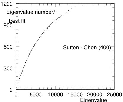
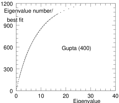
Let the number of eigenvalues less than or equal to be represented by . Now plot the eigenvalue along the x - axis and the corresponding eigenvalue number (in the ordered spectrum) along the y - axis. By definition, this plot is monotonically increasing and is a staircase function that passes through all the points of this plot. Let be the smooth best fit function for this plot. For any finite eigenvalue spectrum is not actually uniquely defined. But for our purposes an approximation maybe made as follows. Generate a suitable function space by combining various elementary functions and using a small number of parameters. The actual construction of the function space is done through the inspection of the data and by trial and error. Now this best fit function maybe generated by varying the parameters in the function space and performing a least square fit. Since the best fit function is known analytically now, we can simply take its derivative and that constitutes our numerically determined DOS function for .
The first key result of this chapter is the following observation. If we exclude about 10% to 15% of all the eigenvalues at both the low frequency and high frequency ends,
can be approximated quite accurately by the functional form for the rest of the spectrum. This observation is applicable to all the four potentials we have studied and also for every system size .
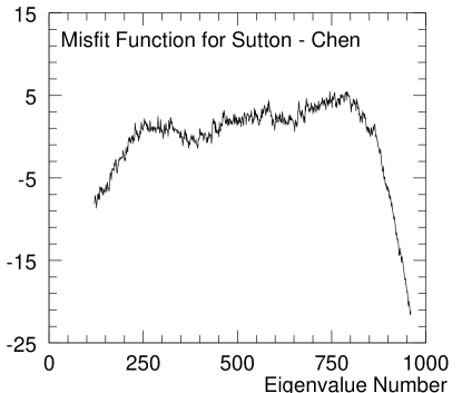
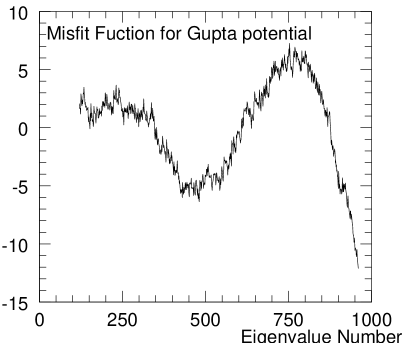
How well does the function approximate ? This question can be answered by defining a misfit function . In the range in which we do the fitting (i.e. excluding 10% to 15% at each end) let be the maximum absolute value of the misfit function as calculated with the best fit values of the parameters a,b and c. Then, if we divide by the total number of eigenvalues within the range of fit, we get an index that can be considered to be an appropriate measure of the accuracy of the approximation. For all the cases that are reported in this chapter, the value of this index stays around or below 0.01. In figures 2.1, 2.3, 2.5 and 2.7 we show how closely the best fit function approximates the integrated density of states. We have taken one sample local minimum with the largest cluster size for each of the four types of potentials. An alternative demonstration is given in figures 2.2, 2.4, 2.6 and 2.8 where we plot the misfit function for the same four local minima.
Before we proceed to perform an analysis of the statistical fluctuations of the eigenvalue spectra, a general comment regarding the density of states function is in order. This is regarding the evolution of the function with the number of particles in the cluster for a given potential. The existence of thermodynamic limit would suggest that will have the structure when is sufficiently large. Here does not depend on the cluster size but should be a function of energy per particle. Given the structure of the function that we are using, will have the form . Thus, and define the scales of and the normalized density of states - both these quantities being, in general, a function of the energy of the local minimum in question. In our case, for a given potential and a given number of particles, the local minima are generated only in a rather narrow range of energy. If we make the standard assumption that the density of states function evolves smoothly with the energy of the local minimum, the implication of
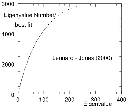
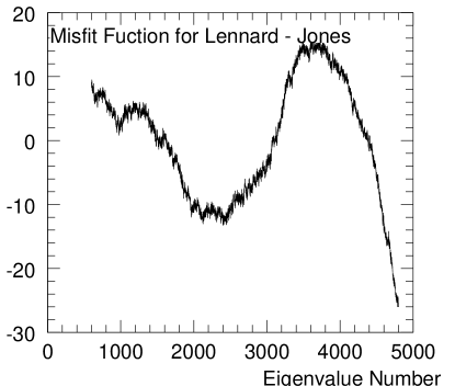
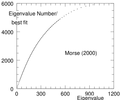
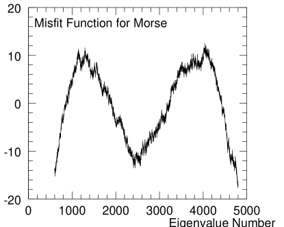
the narrowness of the range of the energies produced is that both and should also be in a correspondingly narrow range. We have computed the mean and the standard deviation of these two parameters and the data is displayed in Table 2.1.
Table 2.1
| Potential | Number of | c | cb/N | s | ||
|---|---|---|---|---|---|---|
| Particles | Average | Standard | Average | Standard | Variance | |
| Deviation | Deviation | |||||
| 200 | 1.60x10⁻² | 6.80x10⁻⁴ | 1.56x10⁻² | 4.02x10⁻⁴ | 0.2844 | |
| LJ | 500 | 1.38x10⁻² | 4.49x10⁻⁴ | 1.37x10⁻² | 2.18x10⁻⁴ | 0.2844 |
| 1000 | 1.26x10⁻² | 2.51x10⁻⁴ | 1.27x10⁻² | 1.34x10⁻⁴ | 0.2852 | |
| 2000 | 1.17x10⁻² | 1.51x10⁻⁴ | 1.20x10⁻² | 8.19x10⁻⁵ | 0.2854 | |
| 200 | 3.63x10⁻³ | 1.43x10⁻⁴ | 3.65x10⁻³ | 9.59x10⁻⁵ | 0.2864 | |
| Morse | 500 | 3.21x10⁻³ | 7.97x10⁻⁵ | 3.29x10⁻³ | 5.07x10⁻⁵ | 0.2844 |
| 1000 | 2.97x10⁻³ | 5.50x10⁻⁵ | 3.09x10⁻³ | 3.29x10⁻⁵ | 0.2857 | |
| 2000 | 2.78x10⁻³ | 3.66x10⁻⁵ | 2.95x10⁻³ | 2.26x10⁻⁵ | 0.2845 | |
| 100 | 1.74x10⁻⁴ | 6.76x10⁻⁶ | 1.71x10⁻⁴ | 6.44x10⁻⁶ | 0.2908 | |
| SC | 200 | 1.65x10⁻⁴ | 4.19x10⁻⁶ | 1.65x10⁻⁴ | 4.34x10⁻⁶ | 0.2882 |
| 300 | 1.60x10⁻⁴ | 3.37x10⁻⁶ | 1.62x10⁻⁴ | 4.25x10⁻⁶ | 0.2833 | |
| 400 | 1.58x10⁻⁴ | 2.70x10⁻⁶ | 1.61x10⁻⁴ | 4.45x10⁻⁶ | 0.2856 | |
| 100 | 1.96x10⁻² | 8.76x10⁻⁴ | 1.86x10⁻² | 8.53x10⁻⁴ | 0.2942 | |
| Gupta | 200 | 1.71x10⁻² | 6.14x10⁻⁴ | 1.63x10⁻² | 3.83x10⁻⁴ | 0.2838 |
| 400 | 1.49x10⁻² | 7.39x10⁻⁴ | 1.46x10⁻² | 2.48x10⁻⁴ | 0.2841 | |
Inspection of this table shows that the standard deviation decreases with increase in the value of in all the cases. Simultaneously, the mean values appear to go to a non - zero limit. This suggests the existence of a well defined density of states function as the number of particles in the cluster becomes very large. For the algorithm that we are using to generate the local minima, we have no direct control over their energies. Thus, the apparent convergence of as well as suggests that the energy per particle goes to some limiting value in the large limit. However, we have no a priori control over this limiting value of the energy per particle.
In order to analyze the statistical fluctuations of the eigenvalue spectra, we use procedures
that are standard in the theory of Random Matrices [69-72]. The first step is to convert the spectrum
of eigenvalues into what is called an “unfolded” spectrum. This is done by using the map
. Given the definition of the function that has been
provided earlier, it is obvious that the average nearest neighbor spacing of the transformed
eigenvalues will be unity everywhere in the spectrum. This standardization of the scale of
spacing makes it possible to compare the nature of fluctuations between different parts of the
same spectrum or two entirely different spectra. One benefit of the process of unfolding is
that the statistics of the analysis of the fluctuations can be significantly improved
by combining the data from many different unfolded spectra if there is reason to believe
that the nature of the statistical fluctuations is the same for all the spectra. However,
it should be kept in mind that the transformation from the raw spectrum to the unfolded
spectrum is implemented by using the function with the best fit values of a,b and
c specific to that local minimum. To summarize the procedure:
(1) Take the ensemble of local minima
generated for a particular potential with a specific number of particles.
(2) Generate the
eigenvalue spectra for all the minima, and
(3) Unfold all the spectra.
On this collection of the unfolded spectra, we perform the following kinds of analysis of
statistical fluctuations:
(1) Calculate the distribution () of the nearest neighbor spacing
.
(2) Define the variable to be the number of levels within a window of length of placed
randomly in the spectrum. Then we calculate variance [], skewness
[]
and excess [] parameters of the distribution of the variable .
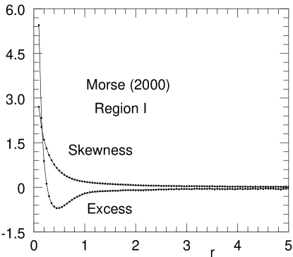
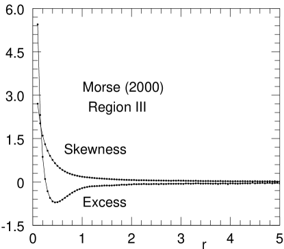
Before we present the data on the statistical analysis, we should reiterate that the approximation to the function holds good only over a large central region of the spectrum. We consistently take this region to be what is left after excluding the lowest 10% and the highest 20% of each spectrum. This is called ‘region II’. We refer to the spectral regions below and above this range as ‘region I’ and ‘region III’, respectively. Analysis of the spectral fluctuations for these two relatively small regions are performed separately whenever they contain adequate number of eigenmodes. We now proceed to present the results of the analysis of the statistical fluctuations for the Lennard-Jones, Morse, Sutton - Chen and Gupta (for nickel) potentials. The largest cluster sizes that we have used with these four potentials are 2000, 2000, 400, and 400, respectively. The reason behind the largest system size being much smaller for Gupta and Sutton - Chen potentials is the presence of the many body terms. This causes a very large increase in the requirement of the computational power. As a result, we are constrained to use much smaller system sizes and fewer local minima as compared to Morse and Lennard-Jones potentials (which are of the form of sum over pairs).
Region II
In this section we present the results of the analysis of statistical fluctuations in the large central region of the spectrum for all the four types of potentials. Analysis of individual spectra suggests that in every case the fluctuations have the characteristics of the Gaussian Orthogonal Ensemble (GOE) of random matrices. However, the quality of the statistics is unsatisfactory owing to the relatively small number of levels in the region II of each spectrum – not exceeding about 4000 in any case. Since all the spectra individually have the features of GOE, we are able to improve statistics by combining the data for all the spectra obtained for a given number of particles with a particular potential.
First of all we present the data for the distribution of the normalized nearest neighbor spacings for the largest cluster size generated with each potential in figures 2.9, 2.10, 2.11 and 2.12. In each of the figures we also show the prediction from the Wigner’s surmise as well as the exact prediction for the GOE [69].
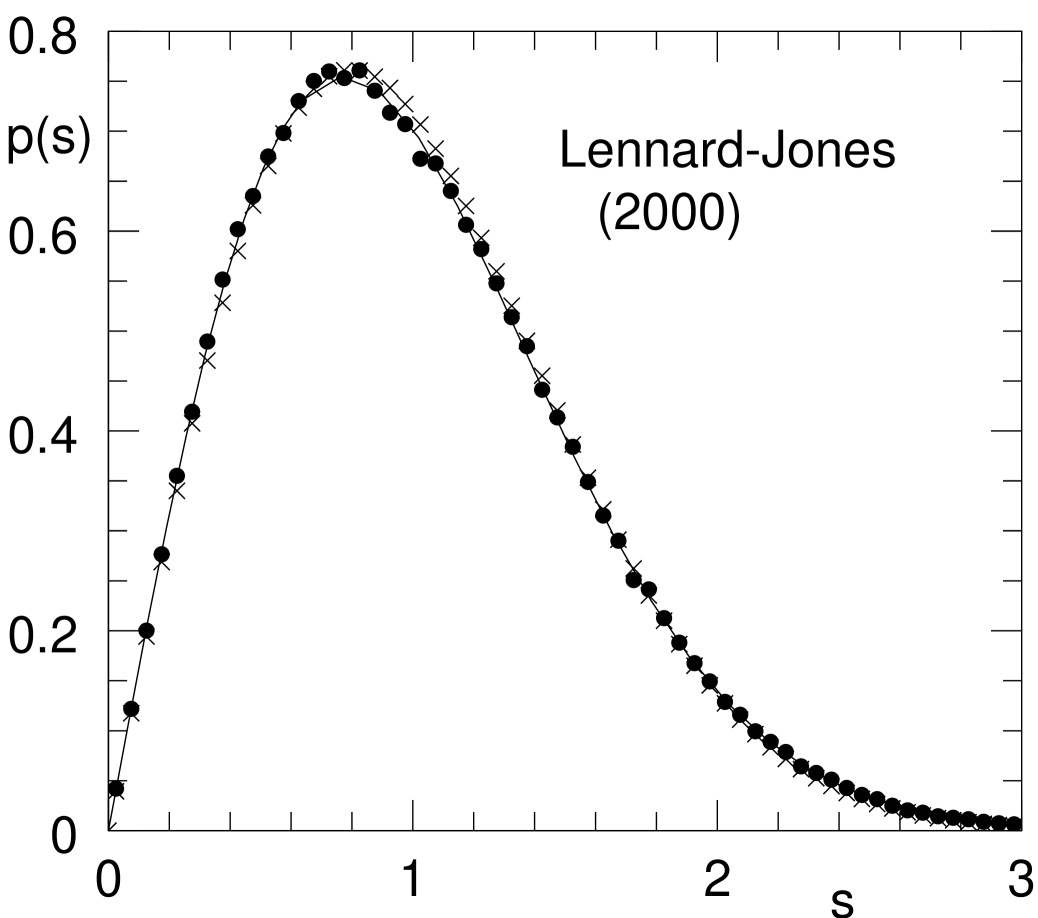
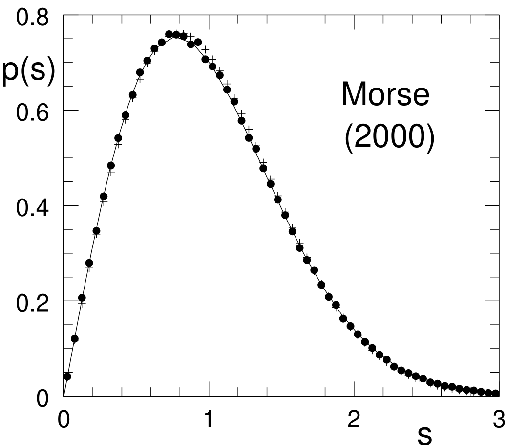
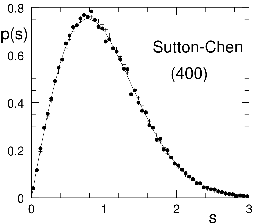
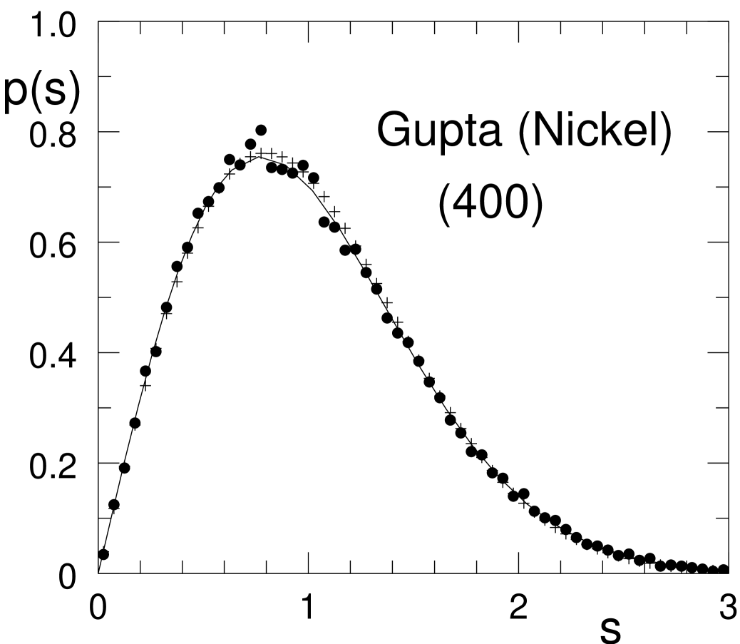
The Wigner surmise is an approximate but highly accurate formula for . Its deviation from the exact prediction is typically of the order of 1% or less and it has been extensively used in the literature. Part of the reason behind this extensive use of a formula that is known to be approximate is that the level of statistics in most applications is simply not large enough to be able to meaningfully distinguish between the approximate formula and the exact result. However, in our case the ensembles for Lennard-Jones potential and Morse potential are large enough (of the order of one million levels) to make it possible to verify in a statistically significant manner whether our data follows the Wigner’s surmise or the exact result. The plots for in figures 2.9 and 2.10 for Lennard-Jones and Morse potential show clearly that our data agrees with the exact predictions for GOE rather than the Wigner surmise.
For the Sutton - Chen and the Gupta potential ( figures 2.11 and 2.12), the data for show a significantly higher level of scatter around the two predictions but it turns out that even for these two cases, the data points fall essentially within the range of permissible statistical fluctuations. For example, the absolute number of data points in a bin near the peak of the curve are about 12000, 19000, 1200 and 2300 for the Lennard-Jones, Morse, Sutton - Chen and Gupta potential, respectively. From this, the level of allowed statistical fluctuation can be computed and we find that the extent of scatter in the actual data is within permissible limits.
A single valued indicator that follows from the function is the variance of the nearest neighbor spacing. We have calculated this parameter also for every ensemble and the results are available in the last column of Table 2.1. From the exact prediction for the GOE, this variance should be 0.286 whereas the Wigner’s surmise leads to the value of 0.273. Inspection of Table 2.1 shows that the computed values of the variance are in much closer agreement with the exact GOE prediction.
We should point out here that the distribution of the nearest neighbor spacing is not too sensitive with respect to the size of the cluster. Even for a system with only about 100 particles, there is very good agreement between the computed function and the predictions (see figures 2.13, 2.14, 2.15 and 2.16).
The significance of this observation is the following:
Any attempt at verifying these predictions in laboratory experiments or ab - initio
calculations will involve only relatively small clusters (of the order of 100 or so)
since bigger sizes are not feasible presently. Thus, it is important that the GOE
properties should be observable even for systems of such small sizes.
Our results for the clusters containing only 100 particles suggest that this is
indeed the case.
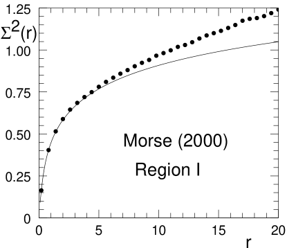
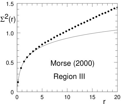
Now we consider the computation of , which is the variance of , the number of levels within a window of length placed randomly in the spectrum. For a credible computation of this characteristic, special care must be taken while unfolding the spectrum. As we have mentioned earlier, the function with appropriately chosen values of a, b, and c does provide a rather close approximation to the ideal smooth function . But an examination of the misfit functions (see figures 2.2, 2.4, 2.6 and 2.8) shows that it is still not close enough as far as the computation of is concerned. Specifically, the misfit functions have an amplitude of fluctuations (around zero) of the order of 1% of the range of the fit and large scale systematic mismatch is apparent. Since the value of for GOE stays around unity, even for fairly large values of , this level of systematic mismatch renders any calculation of variance for large values of unacceptable. For GOE the spectrum is extremely rigid and grows only as . On the other hand, the error in the computation of which is caused by the systematic mismatch that we have mentioned earlier grows proportional to and the constant of proportionality grows with the extent of the mismatch. Hence, it is quite essential that the amplitude of mismatch should be brought down to the lowest possible level and ideally the mismatch function should reflect
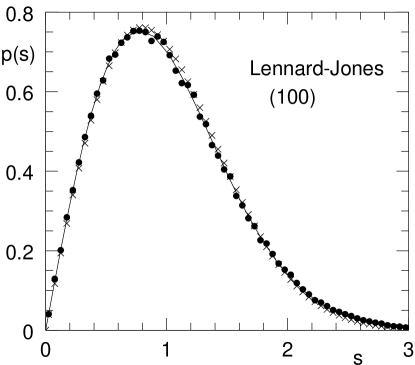
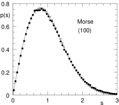
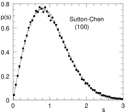
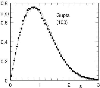
only the statistical fluctuations which are inherent to GOE. In our analysis we have effected a reduction in the amplitude of the mismatch function by adding a correction term to the principal fitting function . To do this we first of all identify the regions of the mismatch function where the behavior is rather irregular. Since there is no simple way to get a smooth fit through these regions they are eliminated from further consideration. For the remaining relatively smooth regions ( which we call ‘accepted regions’) ,which are typically 2 or 3 in number, we separately construct quadratic fits to the mismatch function. Adding these quadratic functions to the principal fitting function , we get the final approximation to for each of the accepted regions separately. Thus, the approximation to which is actually used for unfolding is somewhat different for each of the accepted regions within the same spectrum. We should mention here that all the data for the normalized nearest neighbor spacing that are reported in this thesis are generated from spectra that have been unfolded by using the combined unfolding function – although the function would not be altered recognizably even if we omitted the quadratic correction term in the unfolding function. For the calculation of for a given value of , we use the ensemble of computed for all the accepted regions of all the spectra for a given cluster size and a given potential. This same ensemble is also used for calculation of the skewness [] and excess [] parameters which are defined as
| (2.5) |
| (2.6) |
where is the number of data points in the ensemble for . and are the standard deviation and mean of , respectively.
Data for is displayed for the four potentials in figures 2.17, 2.18, 2.19 and 2.20. In each figure we combine the data for several cluster sizes to exhibit the trend of dependence on
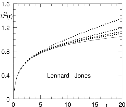
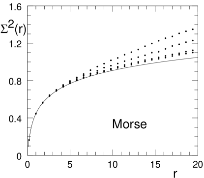
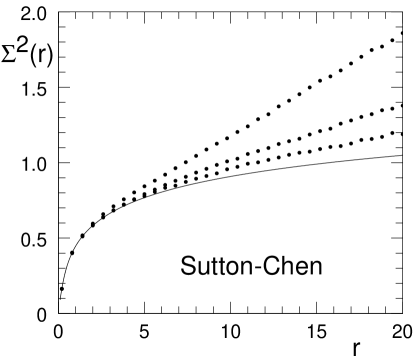
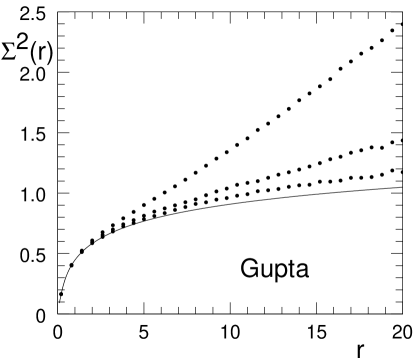
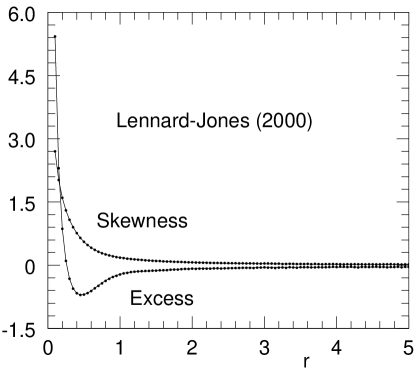
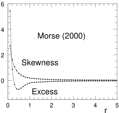
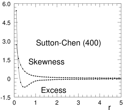
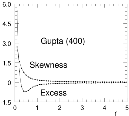
. Common to all the figures is the observation that the agreement between the predictions for the GOE [69] and the computed data becomes closer as the system size increases. Data for the skewness and excess parameters are presented in the figures 2.21, 2.22, 2.23 and 2.24 for the largest system size used with each of the four potentials. In each case the exact predictions for the GOE are also included. These “exact predictions” have been calculated on the basis of a large ensemble of 500 X 500 matrices belonging to the Gaussian Orthogonal Ensemble.
The reason why, for skewness and excess parameters, we show only the data for the largest system size in each case is that there is hardly any detectable dependence on the system size. Even for as small as 100 this is true - as can be seen in the figures 2.25, 2.26, 2.27 and 2.28. Thus, along with the nearest neighbor spacing, skewness and excess parameters form ideal candidates for observing the GOE nature of the fluctuations in possible future experiments and ab - initio calculations. In all the data on and we have included information up to since both these functions become very small in absolute value beyond
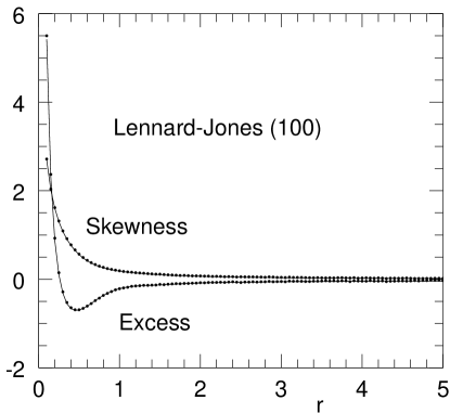
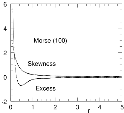
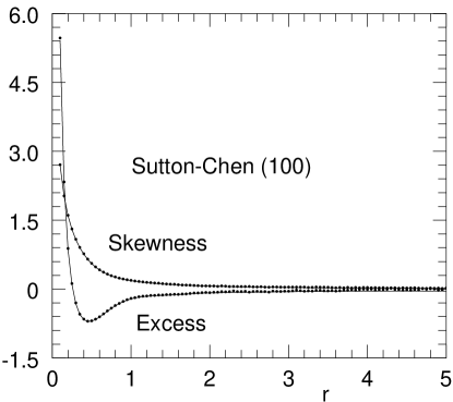
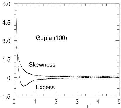
this range. For , the agreement between the predictions for the GOE and our calculations is very close - as can be seen in the figures 2.21 to 2.28. As mentioned earlier, in the procedure adopted for the calculation of , and , we have excluded some regions of spectra where the misfit function has irregular behavior. Although the broad contours of the misfit function are more or less same for all the spectra with a given potential and a given number of particles, the exact locations of these irregular regions do vary somewhat from spectrum to spectrum. However, since we are dealing with a very large number of spectra (of the order of 1000 in some cases) and the exclusion of the irregular regions is done only through visual inspection, we have actually selected the same groups of frequencies for all the spectra after inspecting only a few of them. This process is somewhat subjective (and improper, strictly speaking) and causes some degradation in the quality of unfolding. All the data on that have been presented in figures 2.17, 2.18, 2.19 and 2.20 suffer from this limitation. However, in the cases of Lennard-Jones potential and Morse potential with 2000 particles (the number of spectra being 262 and 49, respectively) we have examined the misfit function for each spectrum separately and excluded the irregular regions accordingly. The results of this analysis for are shown in figures 2.29 and 2.30.
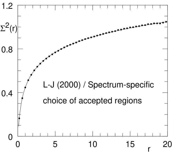
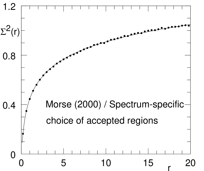
One can see that now there is essentially overlapping agreement with the predictions of GOE all the way up to . This is to be compared with the data in figures 2.17 and 2.18.
Regions I and III
In this section we present the results of the analysis of
statistical fluctuations for the top 20% (region III) and the
bottom 10% (region I) of the spectra. This is done only for
Lennard-Jones and Morse potentials. For the other two potentials
the number of eigenvalues in either of these two regions is too
small to permit any statistically significant analysis – even for
the largest system sizes used. For the Lennard-Jones and Morse cases
the number of levels in these two regions are reasonably high for
the largest system size of . The reasons why we perform
the analysis separately for these two regions are two-fold:
(1) As we have seen earlier, analysis of fluctuations is preceded by the construction of an analytical unfolding function. However, we are unable to construct such a function for the entire spectrum in one go.
(2) We have calculated the participation ratios of the eigenmodes and the values indicate that the modes are extended in a large central part of the spectrum overlapping region II. However, towards the top of the spectra, the eigenmodes are more and more localized and they are completely localized at the top of region III. In the region I the eigenmodes seem to be a mixture of extended and localized type. Since, from literature, we expect a connection between the nature of spectral fluctuations and the localization characteristics of the eigenmodes, it is better to analyze these regions separately so as not to mix up regions with possibly different types of spectral fluctuations [32,66].
As before, we have to make a proper choice of the unfolding function that fits the cumulative density of states data sufficiently closely. We choose this fitting function to be a quadratic function in region I since the range of the fit is rather limited. For region III, the unfolding function has the same form as in region II but with different values of parameters. We remove a further 5% of the spectra from the top of region III and 1% from the bottom of region I in order to make the fit sufficiently close.
Figures 2.31, 2.32, 2.33 and 2.34 show the distribution of the normalized nearest neighbor spacing for the regions I and III with the two different potentials. Also shown in each figure are the two types of theoretical predictions. Inspection of these figures show that the closeness of the numerically computed nearest neighbor spacing distribution to the exact prediction for the GOE is essentially as good as it is for region II. However, on account of the lower level of statistics for regions I and III, scatter of the data around the prediction is somewhat higher than it is for the region II. Thus the deviation from the GOE statistics ,if any, is certainly weak even in those sections of the eigenvalue spectra where localization is much more pronounced. To summarize the results for the spectrum as a whole, any departure from the GOE statistics much be limited to a small fraction of levels at the two ends of the spectrum (five percent at the top and one percent at the bottom). These regions, even for the maximum system sizes we have used, contain such a small number of levels that it is not presently possible to perform an independent study of the spectral fluctuations.
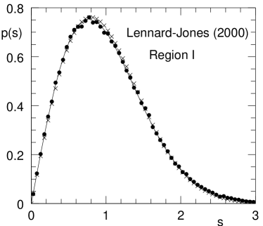
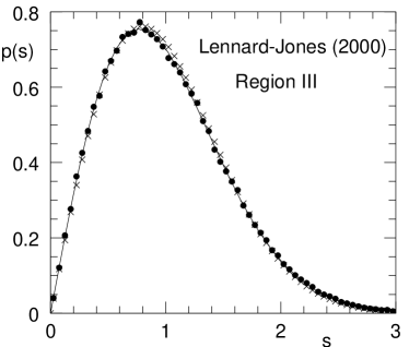
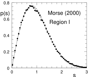
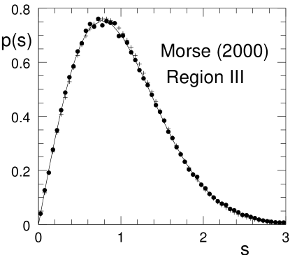
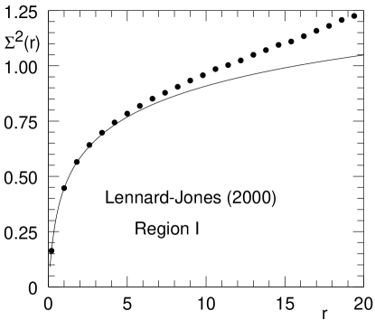
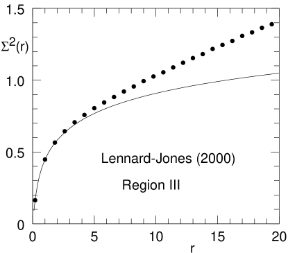
Data for the variance for the two regions and with
the two potentials are presented in figures 2.35, 2.36, 2.37 and 2.38.
It is immediately obvious that the deviation of the numerically computed
values of the variance for the different window lengths from the
exact predictions for the GOE is significantly higher now as compared
to region II – especially when higher values of are considered.
The probable reasons for this higher deviation are:
(1) The quality of the fit of the unfolding function.
(2) The possibility that there is a presence of Poissonian statistics
due to higher level of localization in regions I and III which are
located at the two ends of the spectra.
It is difficult to make a clear statement on the relative importance
of these two probable causes. However, since the agreement of the
nearest neighbor spacing distribution to the prediction for the GOE
is so close, it seems reasonable to conclude that it is the
quality of the unfolding that is the primary reason for the
deviation of variance from the prediction for the GOE. In arriving at
this conclusion we have kept in mind the fact that the nearest neighbor
spacing distribution is much less sensitive to the quality of the process of
unfolding.
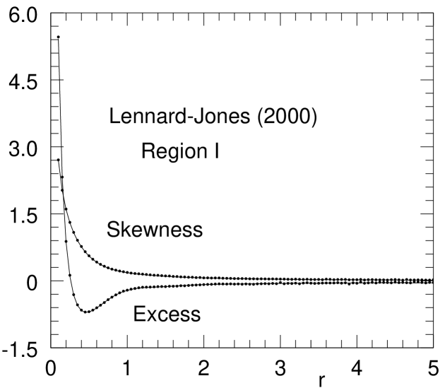
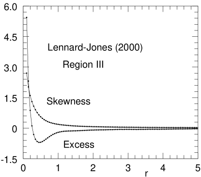
Finally, in figures 2.39, 2.40, 2.41 and 2.42 we display the plots of skewness and excess parameters as a function of window length for the two potentials . Also superimposed are the predictions for the GOE. The closeness of agreement are quite apparent in the figures.
Chapter 3 Universality of Statistical Fluctuations : Binary Amorphous Clusters
In this chapter we continue the study of statistical fluctuations in the vibrational spectra of amorphous systems. But now we consider systems that are made up of two different kinds of constituent units. Studies in chapter 2 showed that for a large central region of the vibrational spectra of single-component amorphous systems, the integrated density of states can be described very accurately by a functional form that does not depend on the nature of the interaction. Also, the spectral fluctuations turned out to be of the GOE type to a very high level of accuracy in all cases. It is natural to ask whether these kinds of universal properties will hold even when the system is more complicated. The simplest situation to which one can extend these investigations is the one pertaining to binary systems. In situations where the potential can be written as a sum over pairs, three functional forms are needed for binary systems corresponding to the three distinct pairs of constituent units that are possible. In our investigation we take a Lennard-Jones type of potential for every pair i.e. the potential for the pair involving two units of type and separated by a distance is given by 4. Thus, the values of and for all the three pairs are needed to completely specify the potential energy of the system for a given configuration. We have studied situations with different ratios of the numbers of the two different kinds of units, different system sizes and different rules for the construction of the Lennard-Jones interaction parameters between the two species. Also the masses of the two types of units are sometimes the same and sometimes different. Here we will present the results for four different situations. Common to all of them are the following: ( Denoting the two types of units as A and B) , and . Here and denote the numbers of units of type and , respectively. The four cases for which we present the results here are specified in Table 3.1 in which and denote the masses of the two types of the units.
Table 3.1
| Case I | 1 | 2/3 | ||
| Case II | 4 | 1.5 | 0.8 | 2/3 |
| Case III | 1 | 1 | ||
| Case IV | 4 | 1.5 | 0.8 | 1 |
It may be noted that in cases I and III, the parameters of the Lennard-Jones potential for the pair with nonidentical units are the same and are constructed via the Lorentz - Berthelot rule. However, the ratios of the masses are different in the two cases. In cases II and IV, the parameters for the nonidentical pair correspond to a choice that has been used extensively in the literature [9-10,12-13]. Here again, the only difference between the cases II and IV comes from the mass ratio.
While generating the random initial configuration for the process of minimization, we assign a type ( or ) to each particle and that completes the definition of the potential. After this the process of generating the local minima is the same as that for a single-component cluster. The construction of the eigenvalue problem is slightly more complicated when the masses of the two units are not identical.
Once the spectra for the various local minima are generated, the rest of the analysis is essentially the same as in the case of a single-component cluster. For example, we find that the functional form fits the cumulative density of states to a very high degree of accuracy in region II. The maximum absolute value of the misfit function stays at the level of 1.5% or less of the range of the fit. Here again, we improve the process of unfolding by adding a quadratic correction to the function for various subdomains of each spectrum. Since our primary interest here is to investigate whether the universal properties observed for single-component clusters are also present for the binary systems, we present results only for the region II and ignore the other parts of the spectrum (i.e. region I and region III).
Figures 3.1 to 3.12 show the data for the nearest neighbor spacing, variance and skewness ( plus excess) for the four cases.
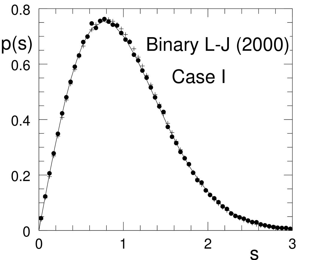
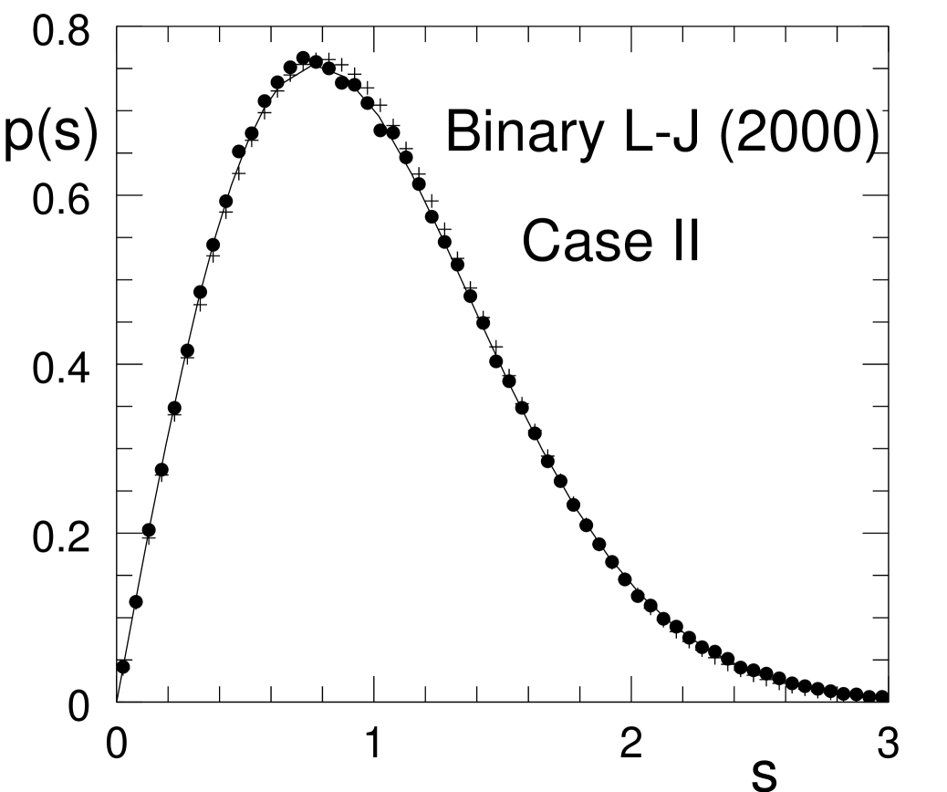
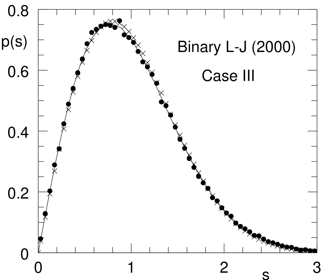
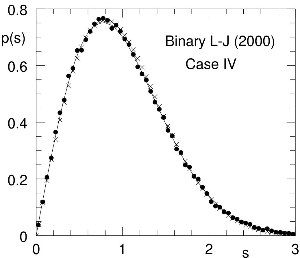
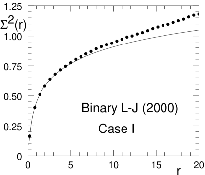
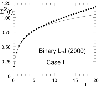
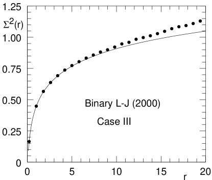
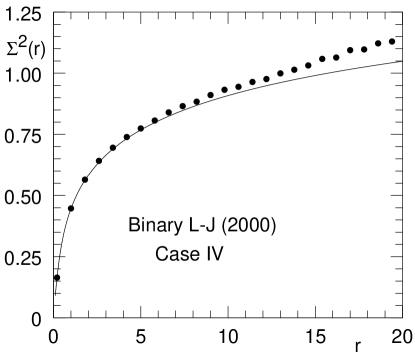
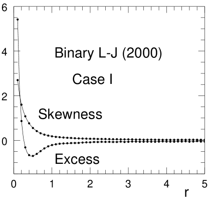
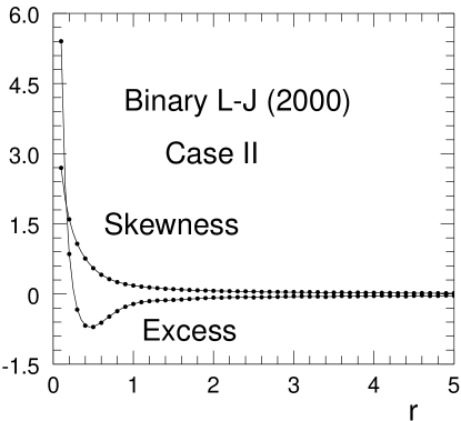
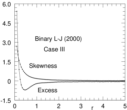
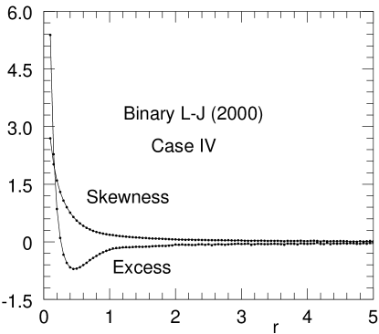
It can be seen that the agreement with the predictions for the GOE is at the same level as that for single component systems as far as the nearest neighbor spacing and skewness ( plus excess ) are concerned. However, in the case of variance () the disagreement with the predictions for the GOE seems to be somewhat higher for larger values of . It is quite likely that this is merely a consequence of not choosing the accepted regions of the spectra separately for each local minimum.
Chapter 4 Universality of the Density of States for Amorphous Clusters
The two previous chapters on the vibrational properties of amorphous clusters have dealt mostly with an examination of the nature of statistical fluctuations in the language of Random Matrix Theories. The first step in such an analysis is the unfolding of the spectrum. Let us recall that we needed a smooth and highly accurate fitting function for the plot of eigenvalue versus eigenvalue number. The analytical form of this fitting function is given by []. This function fitted the cumulative density of states quite closely over the large central region of the spectrum which was labelled as Region II. This was true for all the potentials and all the system sizes that we studied. Note that the function has only one scale () for , namely . This means that if is chosen as the unit of , all the density of states curves can be mapped into a single master curve in the Region II to a rather good approximation - which is what we mean by universality in the density of states. However, since the fit is close only in Region II it is not clear whether the universality extends over the whole spectrum. It is certainly possible, in principle, that there exists a universal fitting function over the entire spectrum but we do not know its functional form and the functional form ( = ) happens to provide a very good approximation to the true underlying universal function in the large central region provided a, b and c are chosen properly. In this chapter we examine this possibility through a numerical analysis of the vibrational spectra. In this connection it is appropriate to remember that for a given potential and a given number of particles, the local minima that correspond to amorphous clusters will be distributed over a range of energies. Of all these possible energies, we obtain the ones that have the largest basin of attraction with respect to our method of generation of local minima. Thus, our procedure permits us to examine the theme of universality over the entire spectrum only for these minima.
Since different potentials will have different scales of frequency , () it is necessary first of all to decide on the appropriate unit of frequency in each case before the density of states functions can be compared. We choose, for any given spectrum, the unit of frequency to be the average frequency of that spectrum. Once the frequencies are normalized in all the spectra corresponding to a given potential and a given number of particles, we can combine the histograms for the normalized frequencies to generate its distribution. The normalized form of the distribution of the normalized frequency () is denoted here by . In figure 4.1 we present the data for the normalized density of states function for six different cases for which the cluster sizes are comparable (400 or 500). This grouping of data according to system size is done keeping in mind the presence of finite size effects. The cases which are shown in figure 4.1 correspond to (with the size of the cluster shown in parenthesis): (1) Single-component Lennard-Jones (500), (2) Morse (500), (3) Sutton - Chen (400), (4) Gupta (400) for nickel, (5) Gupta (400) for vanadium and (6) Binary Lennard-Jones mixture with parameters of Case I of chapter 3 (500). Before normalization of frequency, the maximum values of for these six cases are approximately 16, 33, 150, 18, 5 and 32 respectively.
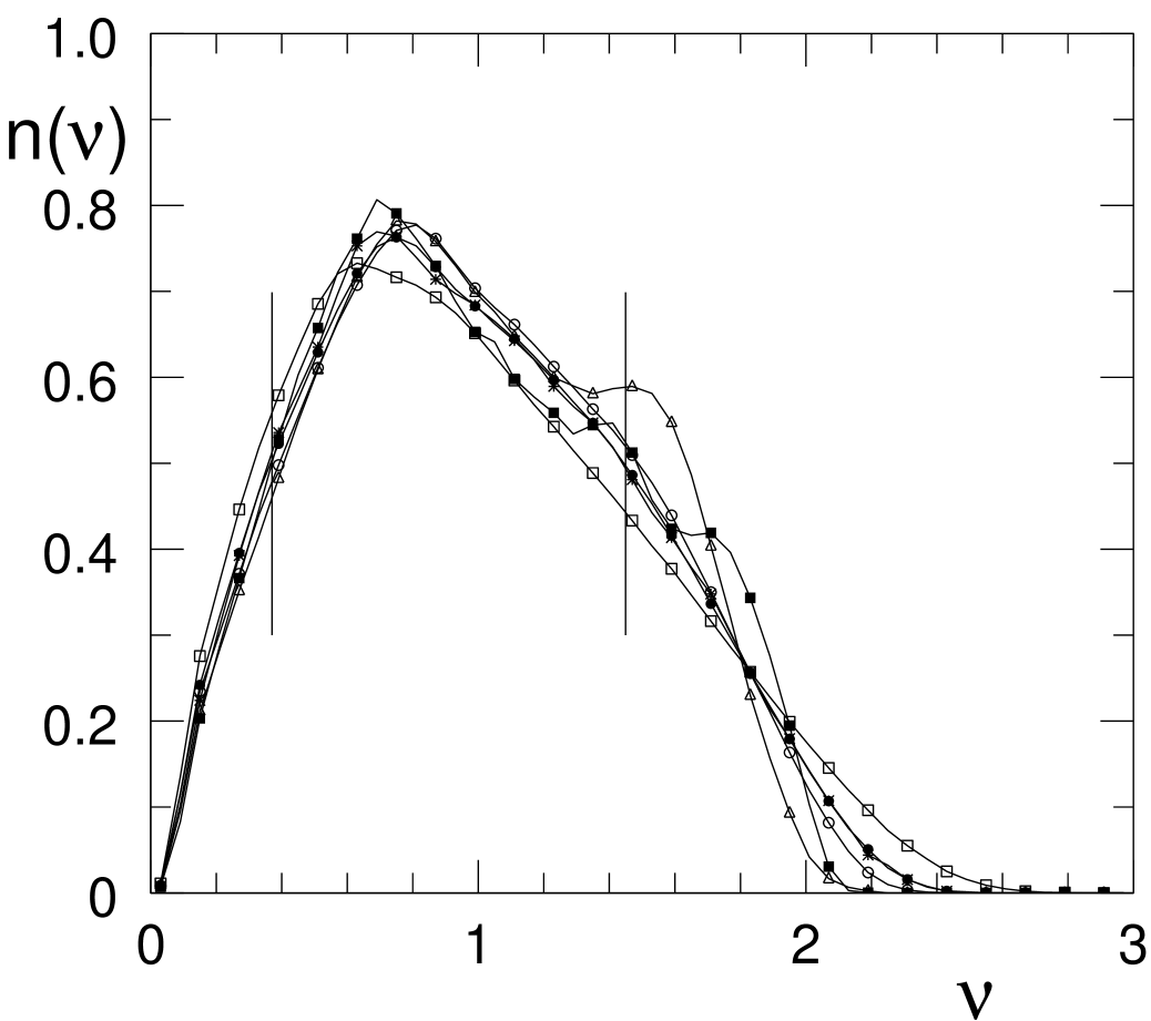

Figure 4.2 shows similar data with the number of particles for: (1) Single - Component Lennard-Jones, (2) Morse, (3) Binary Lennard-Jones, Case I and (4)Binary Lennard-Jones, Case II. The scales of intrinsic frequencies for the six cases in figure 4.1 vary by a factor of almost 30. Given such variations of the intrinsic scales, the extent of overlap of the normalized density of states curves in figures 4.1 and 4.2 is certainly strongly suggestive. But in the light of the observation that the function describes the cumulative density of states to within 1% in Region II, which includes approximately 70% of the spectrum, this apparent overlap of the different normalized density of states functions is somewhat misleading. To demonstrate this, we replot the data of figures 4.1 and 4.2 in figures 4.3 and 4.4 by choosing the unit of frequency to be the inverse of the square root of the best fit value of c – which is the natural scale of frequency suggested by the functional form of . It is obvious from figures 4.3 and 4.4 that the quality of overlap in Region II is much better now.
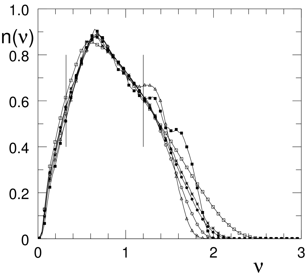

Data presented in figures 4.1, 4.2, 4.3 and 4.4 suggest that the universality of the density of states holds fairly accurately over the large central region of the spectrum but not over the rest of the spectrum. The inclusion of regions I and III, where there is a violation of the universality, while computing the scale of frequency in figures 4.1 and 4.2 causes the significant deviation around any master curve in these two figures. It can also be seen in figures 4.1 and 4.3 that the Sutton - Chen spectrum for nickel and the Gupta spectrum for vanadium contain small but visible peaks in addition to the broad central peak.
To understand these features we need to use a physical insight that was first provided by Rehr and Alben [38] regarding the mechanism of how the sharp peaks of a crystalline spectrum transform into the rather broad peaks of an amorphous solid as more and more disorder is introduced in the system. According to this line of reasoning, the computation of the vibrational spectrum of a disordered system can be divided into two steps. In the first step it is necessary to construct a geometry for the configuration around which the vibration takes place (For us any configuration corresponding to a local minimum of the potential energy function is a candidate). The next step is to construct a model of vibration. This is done by connecting all pairs of elements within an appropriate cut-off distance via linear springs. The spring constants for the pairs within the cut-off distance have a well defined functional dependence on the corresponding pair separation. Thus, the vibrational modes of a solid are computed as the normal modes of this interconnected spring-mass system. Now even if the spring constants for all the pairs included are taken to be the same, the sharp peaks of the crystalline spectrum will still transform to the broad peaks for disordered systems. This is due to the change in the topology of the spring-mass system induced by disorder which changes the connectivity pattern. Thus, this ‘topological disorder’[38] will destroy the van-Hove singularities of the crystalline spectrum but the broad features will still survive – since, even for amorphous states, the local geometry is still substantially like that present in a crystal. Now if we consider a situation in which the spring constants do change from pair to pair according to the pair separation, disorder will introduce another source of broadening the time scales of vibration via the random variability of the pair separation distances. The precise extent of this effect is controlled by the sharpness of the variation of the spring constant with pair separation and is quantified by the third derivative of the potential. This has been referred to as ‘quantitative disorder’[38]. If we keep on increasing the strength of the dispersion of the spring constant, it will ultimately cause the disappearance of even the broad features that resulted from the imposition of only topological disorder. Hence, it is possible to have a spectrum with just one peak in the presence of disorder if the nature of the inter-particle potential is such that there is strong enough ‘quantitative disorder’. This also suggests that if the dispersion of the spring constant is not strong enough, even for disordered systems vibrational spectra may show more than one peak. We believe this to be the explanation for the existence of weak extra peaks in case of Sutton - Chen potential for nickel and Gupta potential for vanadium. Please also note that we are dealing with clusters here and the presence of the surface can be considered to be a source of ‘topological disorder’ – since the elements on the surface will have a different connectivity pattern compared to those in the interior. However, the effect of this ‘topological disorder’ due to finite size will decrease as the cluster size increases since the fraction of elements on the surface will keep decreasing. In that limit more crystalline features will be recovered. For example, the extra peaks in the two cases that we have just discussed are expected to grow in strength as the cluster size increases and this will cause an even stronger violation of universality.
The idea that there may be universality in atleast parts of the vibrational spectra of disordered systems has also been put forward recently on the basis of laboratory experiments with a variety of glasses [65]. These experiments are on bulk systems and the constituent units are too complex to be realistically represented by only the positional degree of freedom. These extra complications will introduce additional features in the vibrational spectra. Nevertheless, if we confine our attention to collective vibrations with coherence length greater than the size of a constituent unit, it will still be permissible to compare the experimental results with theoretical calculations of the type we are considering. The fact that we are dealing with clusters rather than bulk systems will certainly make a quantitative difference. But the main point here is the very existence of universality itself in the vibrational spectra of amorphous systems. To that extent these new experiments put forward the same concept of universality that we have discussed here in the context of clusters. The functional form that has been proposed for the universal density of states function for the bulk glasses is different from what is implied by our function but it also has only one scale of frequency and thus satisfies the necessary condition of shape universality. Infact we have used this functional form also to construct an alternative cumulative density of states function for the purpose of analyzing statistical fluctuations for clusters. To do this please note that the density of states function for in ref.65 is given by . This implies that the cumulative density of states has the form . Now we can repeat the analysis of fluctuations by replacing and [as used in chapters 2 and 3] by and , respectively. The misfit function now has amplitude that is comparable to or somewhat smaller than what is obtained with and . However, this has no quantitative consequence for the analysis of statistical fluctuations since any difference in the quality of unfolding caused by the difference of functional forms at the first level is made up by the process of correction with the quadratic fit to the residue.
It is also possible to study the issue of universality of the density of states function by examining the various moments of the frequency. Let us remember that the information content of the density of states function can be expressed equivalently through the discrete but infinite collection of all the moments. Although we do not presently have a theory for the universality that is observed empirically, it is likely that the preliminary effort in that direction will be in terms of a random matrix type theory which typically concentrates on these moments. We can define these moments both in terms of and but since appears in a somewhat more immediate way in theoretical calculations, we have chosen to calculate the moments of only here. In the present context universality is signalled by the presence of only one scale of in its density of states function. This implies that if we define for every positive integral value of and if universality holds over the entire spectrum, should be universal. We show the data for this ratio of moments in Table 4.1 for the various cases we have studied.
Table 4.1
| Number | |||||
| Potential | of | / | / | / | |
| Particles | |||||
| 100 | 5644.5 | 1.6676 | 3.4641 | 8.1032 | |
| Sutton - Chen | 200 | 5657.8 | 1.6513 | 3.3821 | 7.7913 |
| 300 | 5677.3 | 1.6368 | 3.3139 | 7.5395 | |
| 400 | 5693.4 | 1.6286 | 3.2775 | 7.4116 | |
| Gupta | 100 | 56.9 | 1.8360 | 4.5041 | 13.0656 |
| (Nickel) | 200 | 61.7 | 1.8087 | 4.3018 | 11.9598 |
| 400 | 66.3 | 1.7621 | 4.0328 | 10.7267 | |
| Gupta(Vanadium) | 400 | 7.9 | 1.7034 | 3.6336 | 8.7015 |
| 200 | 261.5 | 1.7452 | 3.9473 | 10.3628 | |
| Morse | 500 | 280.4 | 1.7063 | 3.7216 | 9.3429 |
| 1000 | 291.6 | 1.6825 | 3.5934 | 8.7990 | |
| 2000 | 300.8 | 1.6634 | 3.4933 | 8.3869 | |
| 200 | 62.8 | 1.7968 | 4.2480 | 11.7732 | |
| Lennard-Jones | 500 | 69.0 | 1.7621 | 4.0360 | 10.7592 |
| (Monatomic) | 1000 | 72.7 | 1.7375 | 3.8950 | 10.1187 |
| 2000 | 75.8 | 1.7148 | 3.7687 | 9.5627 | |
| Lennard-Jones | 500 | 195.8 | 1.9088 | 4.9043 | 14.9385 |
| (Binary, Case I) | 1000 | 206.2 | 1.8798 | 4.7182 | 13.9731 |
| 2000 | 214.7 | 1.8558 | 4.5728 | 13.2627 | |
| Lennard-Jones | 1000 | 376.6 | 1.7662 | 4.0473 | 10.7777 |
| (Binary, Case II) | 2000 | 364.2 | 1.7684 | 4.0430 | 10.7030 |
| (L-J Binary, Case III) | 2000 | 250.8 | 1.7539 | 3.9856 | 10.5159 |
| (L-J Binary, Case IV) | 2000 | 389.8 | 1.7463 | 3.9386 | 10.301 |
Please note that the scale of frequency in various situations (as measured by the corresponding average frequency) varies very widely – infact over almost three decades. Second point to be noted is that with increase in the order of moment the high frequency domain of the spectrum plays progressively more dominant role in determining the ratio. Thus, the effect of any deviation from universality in the high frequency domain will be visible more and more in the moment ratio for higher order moments. In Table 4.1 decreases gradually with increase in the system size while keeping the composition, the potential and the value of fixed. However, the signature of convergence is not strong enough . If we focus on the pattern of convergence for the various cases, we cannot draw definite conclusions but the data is also not consistent with the conjecture of universality at this level.
Chapter 5 Universality in the Vibrational Spectra of Bulk Amorphous Systems
In this chapter we address the issue of universality in the vibrational spectra of bulk amorphous systems rather than clusters. In chapter 4 we observed the presence of shape universality over a large central region of the vibrational spectra of clusters with various types of interparticle interactions. The questions we want to address here are: (1) What happens when the system size approaches the bulk limit and (2) Whether there are any situations in which shape universality extends over the entire spectrum rather than over only a large central region.
The methodology that is used to produce the bulk amorphous systems is also used here to address another question which is not a central topic of this thesis but is a rather important issue in its own right. This concerns the presence of ‘boson peaks’ in the vibrational spectra of disordered systems [21-22, 45-65]. This results from the existence of extra modes in the low frequency region of the spectrum. Here by ‘extra’ one means that the density of states is higher than what would be predicted by a Debye type theory based on the speed of sound in the zero frequency limit. Although there are many theories regarding the origin of these extra modes, one aspect to which enough attention has not been paid is to have a detailed and realistic picture of how the build up of the modes in the low frequency region (as well as in the high frequency region) takes place as one goes from the crystalline ground state to the amorphous states. It may be remembered that crystalline vibrational spectra have sharp peaks and van-Hove singularities whereas amorphous states don’t have such features. Here we generate a detailed description of this morphological change in the spectra through a numerical study in which we can create stable solid structures with variable amounts of disorder i.e. any solid structure ranging from perfect crystal to completely amorphous solids. We check our results regarding the evolution of the vibrational spectrum with the predictions of some existing theoretical works in which disorder itself is modelled in a specific fashion [85-90]. In contrast, we model only the interaction between the particles. Disorder follows naturally from it and does not have to be modelled separately.
To generate stable solid structures with variable extent of disorder the first step is to select a model for the interaction among the constituent units (atoms or molecules). Here we assume that every unit has only a position vector as its degree of freedom and the potential energy of the system is of the form of sum over pairs. The route to generating amorphous structures which, strictly speaking, have no periodicity on any length scale is actually via crystalline structures. Let us denote the number of constituent units per primitive cell by . Ideally, should be infinity to produce systems with finite disorder. In practice, however, one takes as large a value as possible within the available computational resources. Now let us denote the three edges of the unit cell by , and . The positions of the particles within the unit cell can be defined by with the values of , and being all between 0 and 1 for every value of . For economy of notation, we denote the triad by .
In order to generate states with variable amount of disorder we begin with a fcc lattice for which the lattice constant is adjusted to minimize the potential energy. Now this system is subjected to a type Monte-Carlo simulation. Here , and represent the number of particles per unit cell, pressure and temperature, respectively, and are held constant during the simulation in which the variables are , and (which define the geometry of the unit cell) and the s for all the particles. In the present calculation we have taken and thus the potential energy per unit cell () constitutes the Hamiltonian of the system. At the end of every m (typically 2) cycles of the simulation, we take the instantaneous configuration and subject it to a conjugate gradient minimization for with respect to , , and all the s [84]. We repeat the process of generating the local minima with various values of the seed of the random number generator in the Monte-Carlo simulation. Finally, the information regarding this collection of solid structures is displayed in the form of a volume per particle () versus energy per particle () diagram.
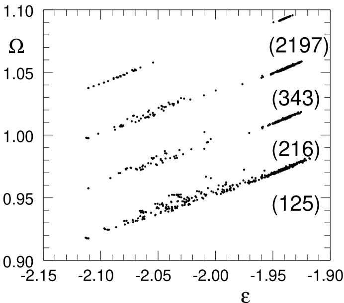
Figure 5.1 provides an example of this kind of volume versus energy diagram for the standard Lennard-Jones potential [ i.e. ] which has been properly cut off and smoothed so that the function as well as all derivatives upto second order are continuous for all values of r. In figure 5.1 the completely amorphous states correspond to the group at the highest energies. Isolation of this group from the rest of the minima is visible more and more clearly as the number of particles in the unit cell increases. This is due to the progressively decreasing probability of generating states in the domain of energies just below the amorphous group as the number of particles in the unit cell increases. For the purpose of demonstrating the evolution of the vibrational spectrum with disorder, these minima are of critical importance. Any calculation such as ours will naturally generate only a small subset of all the local minima that exist. In particular, the data shown in Figure 5.1 certainly do not correctly represent the relative densities of the local minima except in the completely amorphous band.
For the amorphous band the functional dependence of the relative density of the local minima on the value of energy per particle () is given by a Gaussian function whose width is proportional to . This follows from the extensivity property of the configurational entropy and has been observed earlier also in calculations with constant density. It should be noted that our calculations are done under the condition of constant ‘inherent’ pressure. For a given value of energy per particle, dispersion in the value of volume per particle is expected to go to zero in the thermodynamic limit. For the amorphous band we have verified the validity of this observation in our case in the following manner: Compute the best fit quadratic function through the data points in the amorphous band of the diagram. Then calculate the root mean square deviation of from the best fit curve. We find that this measure of scatter around a smooth curve indeed goes to zero in the completely amorphous band as .
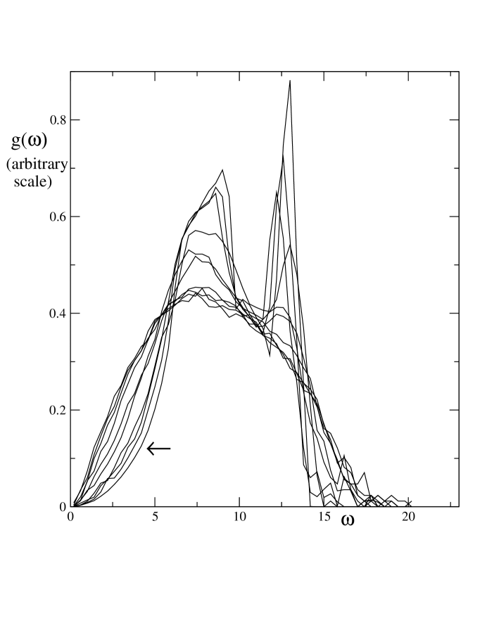
For any local minimum in the plane the associated vibrational spectrum can be computed through standard methods. As energy per particle increases the system becomes more and more amorphous and the density decreases i.e. there is swelling in the system. At the same time there is a continuous change in the nature of the associated vibrational spectrum. Figure 5.2 illustrates this for the case of Lennard-Jones potential with . Here we have picked, from figure 5.1, a few local minima which are spaced roughly equally in energy. For the selected minima we calculate the vibrational spectra and the density of states for each case is plotted in figure 5.2. One can clearly see a gradual transformation from a crystal-like spectrum to one which is characteristic of amorphous states.
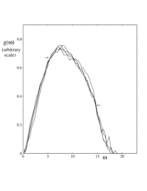
We can compare the data available in this figure with the results presented by Mattis and coworkers for some model calculations on the evolution of the density states as the strength of disorder changes [85-90]. These calculations are for a quantum mechanical model of vibration in which a specific model term is included in the Hamiltonian to describe the effect of disorder. The amplitude of this term quantifies the strength of disorder. It so happens that the spectrum for the model becomes unstable when the strength of the disorder exceeds a critical value. To avoid this it is technically necessary to include an anharmonic term in the Hamiltonian – although, at the end, the strength of anharmonicity can be made arbitrarily small. On the other hand, we use harmonic approximation to compute the normal modes of a classical disordered solid and no explicit model of disorder is needed. To compare the results of our calculation regarding the evolution of the vibrational spectrum with disorder with previous theoretical calculations , it is useful to summarize the main results of these latter calculations.
For a simple cubic lattice, they are the following [90]: (1) For any finite value of the disorder parameter there are no van-Hove singularities. (2) As the strength of the disorder parameter increases, more and more modes are transferred to the domains with the lowest and highest frequencies. (3) There is a critical value of the disorder parameter which marks the boundary between finite long range order [disordered crystal] and vanishing long range order [glass]. When the disorder parameter exceeds this value the density of states function develops two fixed points i.e. there are two frequencies and where the value of the density of states function does not change with change in the value of the disorder parameter. The value of , the higher of the two frequencies, is approximately 3.5 times the value of . (4) When the disorder parameter exceeds the critical value, the value of the density of states function at zero frequency becomes finite and increases with disorder.
While comparing the predictions listed in the previous paragraph with our results, two limitations must be kept in mind. (1) Our starting crystal has a face centered cubic lattice rather than a simple cubic lattice. (2) As we have noted earlier, modelling any finite extent of disorder requires the size of the unit cell to go to infinity, strictly speaking. In our case, the value of is only 343. Despite these limitations, we find that our data is consistent with the first two predictions. Also, if we examine only those spectra in figure 5.2 which correspond to completely disordered states (shown separately in figure 5.3), we notice the presence of two approximate fixed points. However, the ratio is close to 2.4. The fact that it is substantially different from the value of 3.5 obtained in the analytical calculation may be due to the difference between the starting crystal structures of the two calculations. However, our data certainly does not corroborate the fourth prediction of finite value of the density of states function in the limit. We always find that the density of states goes to zero as .
Now we address the central problem of this chapter. The question here is: Are there any situations where, for bulk amorphous systems, the vibrational density of states function assumes a shape that is universal over the entire spectrum? This question is motivated partially by our observations regarding the universality of the shape of the spectrum (but only in the large central region) for the cases of clusters interacting via several different kinds of potentials – as reported in the previous chapters [67-68]. The other motivation behind these investigations is to understand the aspect of universality observed for the density of states function in recent experiments with bulk molecular glasses [65] – as noted in chapter 4. In these experiments the constituent units are too complicated to be adequately modelled as single particles. However, for vibrational modes with coherence lengths much larger than nearest neighbor spacing, replacing a somewhat complicated constituent unit by a point particle may not be a bad approximation. Our approach to discovering the possible situations in which there will be universality in the shape of the entire vibrational spectrum is influenced by the discussion ( see chapter 4 ) of the effect of the dispersion of the second derivative of the potential energy function around its minimum. Let us recall that, according to the insight provided by the work of Rehr and Alben [38], in the limit of the dispersion of the spring constant becoming very large, we expect only a single broad peak in the density of states function. In our calculations the geometries around which vibration takes place correspond to the local minima of the potential energy function. For such a configuration the significant pair distances will largely be distributed around the minimum of the pair potential. Thus, a quantitative dimensionless measure of the dispersion of the spring constant (DSC) is given by where is the distance at which the pair potential assumes its minimum value. Thus, is the limit where we expect a featureless spectrum with a single broad maximum. The numerical data reported later in this chapter is indeed consistent with this expectation. But what is more important and interesting is the following: If the manner in which approaches infinity satisfies an additional condition (to be stated shortly), the vibrational spectrum approaches a shape that is universal to within the uncertainities of our numerical calculation. Here the property of universality implies that the asymptotic shape of the vibrational spectrum does not depend on the analytical form of the potential energy function whose parameters are varied appropriately to realize the limit.
It is possible, in principle, to construct many parametric functional
forms which, with suitable variation of the parameters, can be made to
approach
the limit. We have used only exponential and
power law functions in our parametric functional forms since interatomic
or intermolecular forces will typically have rapid spatial variation
and the only elementary functions that are capable of describing such
variations are the exponential and power law functions. The two types
of functional forms that we have actually used are as follows:
(1) The Generalized Lennard-Jones (GLJ) family where the pair potential
has the form where and are
positive integers with .
(2) The Morse family in which the potential has only one parameter
and the expression is given by .
The overall shape of the pair potential is largely the same for both the
types. They always have a single minimum where the potential function
assumes a negative value. The function rises rapidly to zero at
larger distances. At shorter distances also the potential rises fast but
to a finite value for the Morse case and to infinity for the GLJ case.
In the Morse case the rapidity with which the potential increases away
from the minimum is controlled by the single parameter .
However, for the the GLJ type the rise of the attractive and repulsive
sides are controlled separately by and , respectively. It is easy
to verify that the DSC parameter () is given by () and
for the GLJ and Morse families, respectively.
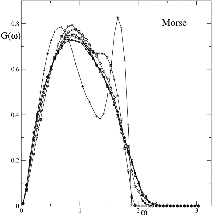
Obviously, for the GLJ case there is no unique sequence for approaching the limit even under the restriction of . Here, either only can go to infinity or both and can go to infinity while always satisfying . Our observation is that only when both and go to infinity, universal shape of the vibrational spectrum is realized i.e. while the dispersion of spring constant goes to infinity, contribution must come both from the attractive and the repulsive sides of the minimum.
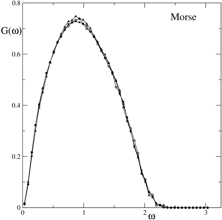
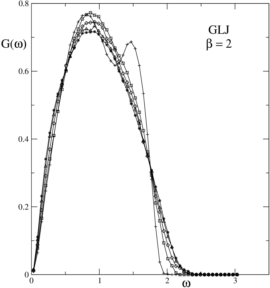
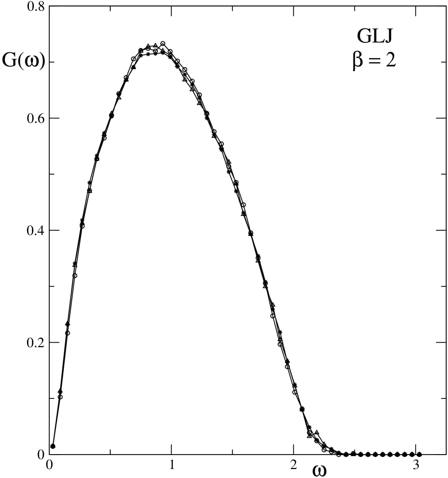
We have already described how to generate the completely disordered states for any given potential. Ofcourse they span a range of energies and there is variation of the vibrational spectrum with energy. Thus, a pertinent question is: which vibrational spectra should be considered representative of these band of states? We use the criterion of maximum likelihood of physical relevance. Thus, for each potential, we calculate the mean and the standard deviation of energy in the completely disordered region. Next, we choose a set of 10 local minima which are approximately equally spaced in energy in the band contained within one standard deviation of the mean. For each local minimum, the spectrum is computed and the frequencies are rescaled so that the average frequency is unity. We then calculate the distribution of these normalized frequencies and average the distribution over the 10 local minima. Finally, this averaged histogram is rescaled to compute the normalized density of states () for normalized frequencies. Figure 5.4 shows the result of such calculation for a series of potentials belonging to the Morse family and figure 5.5 displays the data with the three highest values of so as to show the pattern of convergence more clearly. For the GLJ family, the route to has been taken to be of two different types characterized by the value of for each potential. Here, ofcourse keeps increasing but the value of is taken to be either 2 or 4. The spectra for are presented in figure 5.6 with figure 5.7 showing the cases corresponding to the three largest values of – the idea being again to show the pattern of convergence.
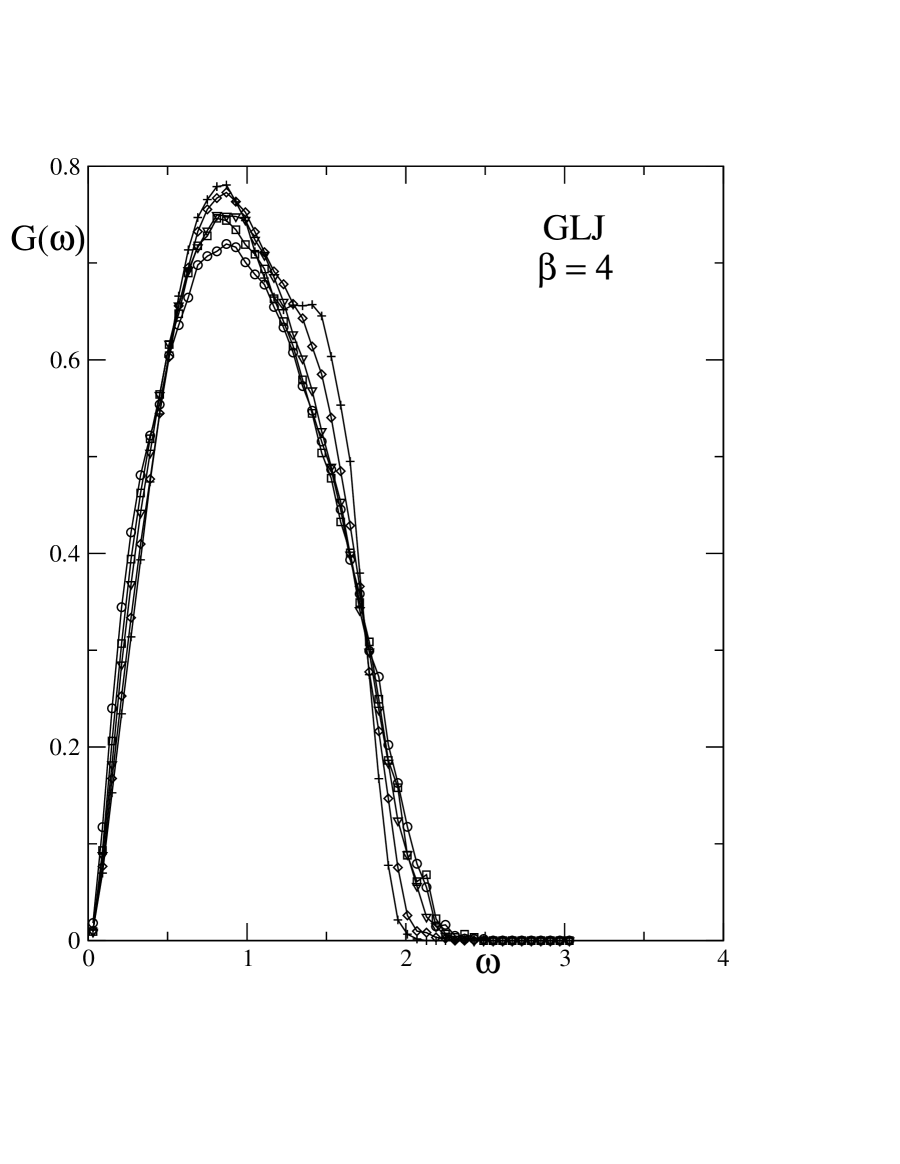
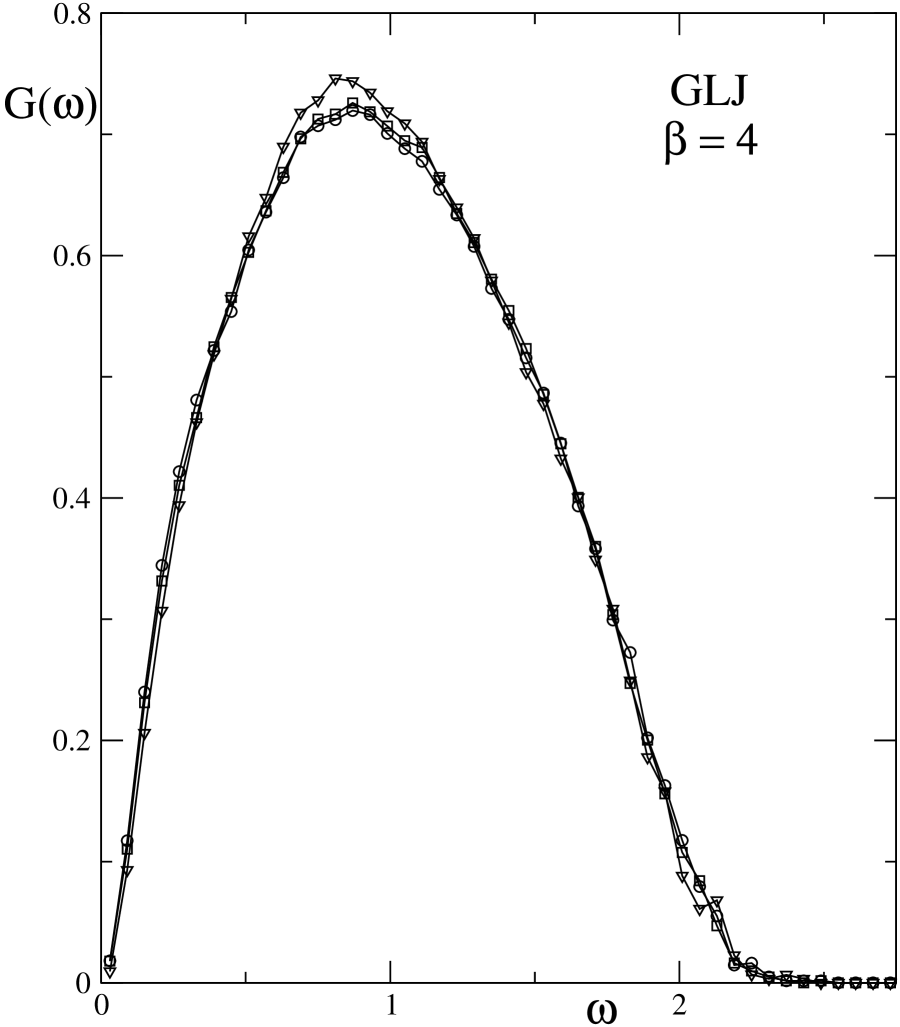
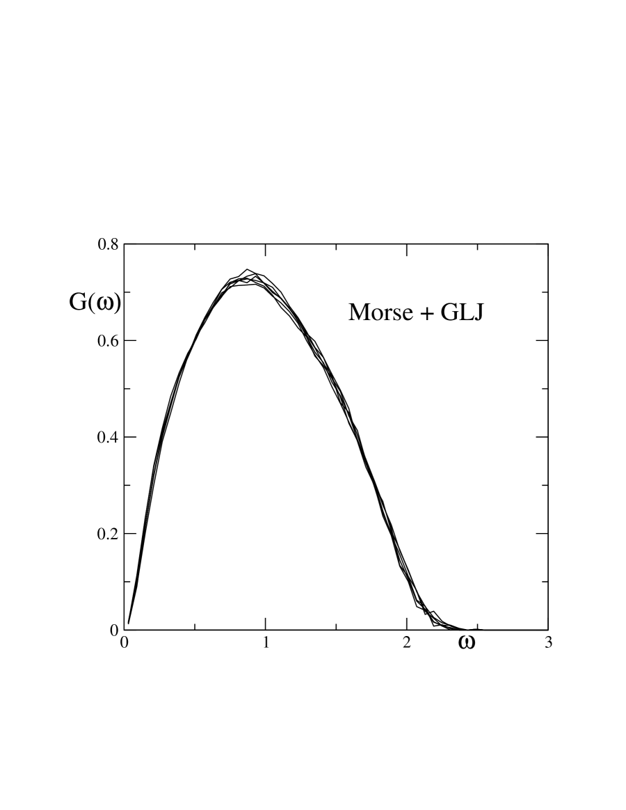
For the sake of completeness, we also present the data for in figures 5.8 and 5.9. Please note that the highest value of that is used is 22 for both or 4. But since corresponds to the highest value of n, in figure 5.10 we superimpose the data for the three highest values of in the Morse family and the three highest values of in the GLJ family with to show the relationship between the asymptotic normalized spectra for the two families. Within the error bars of our calculations, estimated by the standard deviation of normalized density of states in each bin with respect to the 10 local minima in each case, the asymptotic normalized density of states function seem to be identical over the entire spectrum. This is the most important result of this chapter. To restate it, asymptotic density of states is independent of the explicit form of the parametric potential function which is used to achieve the asymptotic limit provided both the attractive and repulsive sides of the minimum of the pair potential contribute to the approach of to infinity.
If we assume the validity of the observation at the end of the previous
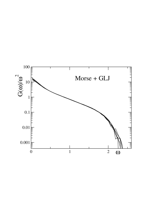
paragraph, an empirical explanation of the observation of universality in the trans-boson peak region of the vibrational spectra of several molecular glasses that has been observed recently emerges. In these experiments [65] it was observed that the semilogarithmic plot of as a function of is a straight line in the trans-boson peak region for several different kinds of glasses. This implies the following functional form of : where is the scale of frequency specific to the material. Our empirical explanation of this observation has to do with two facts: (1) The existence (or presumption) of the asymptotic universal density of states and (2) Change in the vibrational spectrum with the variation of parameter(s) becomes rather weak significantly before asymptotic conditions are reached. Thus, a large family of potentials will have vibrational spectra (in the amorphous region) that is close to, but not quite, universal. Since we do not know the exact nature of the potential function for the specific materials, it is not possible to make a precise comparison with our calculations. The next best course of action is to check whether our asymptotic and (presumably) universal density of states has the functional form seen in the experiments. In figure 5.11 we show a semi-logarithmic plot of the asymptotic normalized density of states (divided by ) against . There is a substantial linear segment in the middle in common with the experimental observations [65]. From our discussion and also from the data presented for both the Morse family and the GLJ family for smaller values of , it should be clear that if the material at hand is described by a potential which is far from satisfying the asymptotic conditions, the vibrational spectrum will not be universal and can even show more than one peak.
The asymptotic universality which is suggested by our numerical results poses a major theoretical challenge. At this moment, we have no understanding of this empirical observation.
Bibliography
-
1.
S. -K. Ma, Modern Theory of Critical Phenomena (Benjamin / Cummings, Reading, 1976).
-
2.
M. Goldstein, J. Chem. Phys. 51, 3728 (1969).
-
3.
T. B. Schrøder, S. Sastry, J. C. Dyre, and S. Glotzer, J. Chem. Phys. 112, 9834 (2000).
-
4.
A. Cavagna, Europhys. Lett. 53, 490 (2001).
-
5.
G. Adams and J. H. Gibbs, J. Chem. Phys. 43 , 139 (1965).
-
6.
F. H. Stillinger and T. A. Weber, Phys. Rev. A 25 , 978 (1982).
-
7.
F. H. Stillinger and T. A. Weber, Science 225 , 983 (1984).
-
8.
F. H. Stillinger, Science 267 ,1935 (1995).
-
9.
S. Sastry, P. G. Debenedetti, and F. H. Stillinger, Nature (London) 393 , 554 (1998).
-
10.
S. Sastry, Nature (London) 409 , 164 (2001).
-
11.
C. A. Angell, J. Non-Cryst. Solids 131-133 ,13 (1991).
-
12.
W. Kob and H. C. Andersen, Phys. Rev. Lett. 73 , 1376 (1994).
-
13.
F. Sciortino, W. Kob, and P. Tartaglia, Phys. Rev. Lett. 83 ,3214 (1999).
-
14.
K. K. Bhattacharya, K. Broderix, R. Kree, and A. Zippelius, Europhys. Lett. 47 , 449 (1999).
-
15.
S. Büchner and A. Heuer, Phys. Rev. Lett. 84 , 2168 (2000).
-
16.
R. A. Denny, D. R. Reichman, and J. -P. Bouchaud, Phys. Rev. Lett. 90 ,025503 (2003).
-
17.
W. Kob, F. Sciortino, and P. Tartaglia, Europhys. Lett. 49 ,590 (2000).
-
18.
K. Broderix, K. K. Bhattacharya, A. Cavagna, A. Zippelius, and I. Giardina, Phys. Rev. Lett. 85 , 5360 (2000).
-
19.
L. Angelani, R. Di Leonardo, G. Ruocco, A. Scala, and F. Sciortino, Phys. Rev. Lett. 85 , 5356 (2000).
-
20.
P. Shah and C. Chakravarty, Phys. Rev. Lett. 88 , 255501 (2002).
-
21.
Special issue of Physica (Amsterdam) 107D, Issue 2-4 (1997).
-
22.
Proceedings of 7th International Workshop on Disordered Systems, Molveno, Italy, edited by A. Fontana and G. Viliani [ Philos. Mag. 79 (1999)].
-
23.
R. J. Bell, Reports on Progress in Physics 35, 1315 (1972).
-
24.
S. R. Elliott, Physics of Amorphous Materials (Longmans, New York,1990), 2nd ed.
-
25.
M. Sampoli, P. Benassi, R. Eramo, L. Angelani, and G. Ruocco, J. Phys. : Cond. Matt. 15 , S1227 (2003).
-
26.
G. Ruocco, F. Sette, R. Di Leonardo, G. Monaco, M. Sampoli, T. Scopigno, and G. Viliani, Phys. Rev. Lett. 84, 5788 (2000).
-
27.
A. Cavagna, I. Giardina, and G. Parisi, Phys. Rev. Lett. 83,108 (1999).
-
28.
T. S. Grigera, A. Cavagna, I. Giardina, and G. Parisi, Phys. Rev. Lett. 88, 055502 (2002).
-
29.
E. La Nave, S. Mossa, and F. Sciortino, Phys. Rev. Lett. 88 , 225701 (2002).
-
30.
S. Mossa, E. La Nave, H. E. Stanley, C. Donati, F. Sciortino, and P. Tartaglia, Phys. Rev. E 65 , 041205 (2002).
-
31.
S. Mossa, E. La Nave, P. Tartaglia, and F. Sciortino, J. Phys. : Cond. Matt. 15 , S351 (2003).
-
32.
P. Carpena and P. Bernaola-Galvan, Phys. Rev. B 60, 201 (1999).
-
33.
G. Parisi, cond-mat/0301282.
-
34.
M. Mézard, G. Parisi, and A. Zee, cond-mat/9906135.
-
35.
A. Fielicke, A. Kirilyuk, C. Ratsch, J. Behler, M. Scheffler, G. von Helden, and G. Meijer, Phys. Rev. Lett. 93 , 023401 (2004).
-
36.
L. V. Heimendahl and M. F. Thorpe, J. Phys. F: Metal Physics. 5, L87 (1975).
-
37.
A. Rahman, M. J. Mandell, and J. P. McTague, J. Chem. Phys. 64, 1564 (1976).
-
38.
J. J. Rehr and R. Alben, Phys. Rev. B 16, 2400 (1977).
-
39.
J. -B. Suck, H. Rudin, H. -J. Güntherodt, and H. Beck, J. Phys. C: Solid State Physics, 14, 2305 (1981).
-
40.
S. R. Nagel, G. S. Grest, S. Feng and L. M. Schwartz, Phys. Rev. B 34, 8667 (1986).
-
41.
K. Vollmayr, W. Kob, and K. Binder, J. Chem. Phys. 105 , 4714 (1996).
-
42.
S. N. Taraskin and S. R. Elliott, Phil. Mag. B 79, 1747 (1999).
-
43.
A. F. Ioffe and A. R. Regel, Prog. Semicond. 4, 237 (1960).
-
44.
P. B. Allen, J. L. Feldman, J. Fabian, and F. Wooten, Phil. Mag. B 79, 1715 (1999).
-
45.
Amorphous Solids: Low Temperature Properties, edited by W. A. Philips (Springer-Verlag, Berlin, 1981).
-
46.
U. Buchenau, N. Nücker and A. J. Dianoux, Phys. Rev. Lett. 53, 2316 (1984).
-
47.
F. J. Bermejo, J. Alonso, A. Criado, F. J. Mompeán, J. L. Martínez, M. García-Hernández, and A. Chahid, Phys. Rev. B 46 , 6173 (1992).
-
48.
V. A. Luchnikov, N. N. Medvedev, Y. I. Naberukhin, and V. N. Novikov, Phys. Rev. B 51 , 15569 (1995).
-
49.
B. Fultz, C. C. Ahn, E. E. Alp, W. Sturhahn, and T. S. Toellner, Phys. Rev. Lett. 79 , 937 (1997).
-
50.
C. A. Tulk, D. D. Klug, E. C. Svensson, V. F. Sears, and J. Katsaras, Appl. Phys. A [Suppl.] 74 , S1185 (2002).
-
51.
M. A. Parshin, C. Laermans, D. A. Parshin, and V. G. Melehin, Physica B 316-317 , 549 (2002).
-
52.
M. A. Ramos, C. Talón, R. J. Jiménez-Riobóo, and S. Vieira, J. Phys.: Cond. Matt. 15 , S1007 (2003).
-
53.
N. V. Surovtsev, S. V. Adichtchev, E. Rössler, and M. A. Ramos, J. Phys.: Cond. Matt. 16 , 223 (2004).
-
54.
O. Pilla, S. Caponi, A. Fontana, J. R. Concalves, M. Montagna, F. Rossi, G. Viliani, L. Angelani, G. Ruocco, G. Monaco, and F. Sette, J. Phys.: Cond. Matt. 16, 8519 (2004).
-
55.
W. Schirmacher, G. Diezemann, and C. Ganter, Phys. Rev. Lett. 81 , 136 (1998).
-
56.
W. Schirmacher, G. Diezemann, and C. Ganter, Physica (Amsterdam) 284-288B ,1147 (2000).
-
57.
V. L. Gurevich, D. A. Parshin, and H. R. Schober, JETP Lett. 76, 553 (2002).
-
58.
V. L. Gurevich, D. A. Parshin, and H. R. Schober, Phys. Rev. B 67, 094203 (2003).
-
59.
T. S. Grigera, V. Martín-Mayor, G. Parisi, and P. Verrocchio, Phys. Rev. Lett. 87 , 085502 (2001).
-
60.
T. S. Grigera, V. Martín-Mayor, G. Parisi, and P. Verrochio,Nature(London) 422 , 289 (2003).
-
61.
T. S. Grigera, V. Martín-Mayor, G. Parisi, and P. Verrochio, J. Phys.: Cond. Matt. 14, 2167 (2002).
-
62.
S. N. Taraskin, Y. L. Loh, G. Natarajan, and S. R. Elliott, Phys. Rev. Lett. 86 , 1255 (2001).
-
63.
S. N. Taraskin and S. R. Elliott, Phys. Rev. B 56, 8605 (1997).
-
64.
C. A. Angell, Y. Yue, L. -M. Yang, J. R. D. Copley, S. Borick, and S. Mossa, J. Phys.: Cond. Matt. 15 , S1051 (2003).
-
65.
A. I. Chumakov, I. Sergueev, U. van Bürck, W. Schirmacher, T. Asthalter, R. Rüffer, O. Leupold and W. Petry, Phys. Rev. Lett. 92, 245508 (2004).
-
66.
S. Sastry, N. Deo, and S. Franz, Phys. Rev. E 64, 016305 (2001).
-
67.
S. K. Sarkar, G. S. Matharoo, and A. Pandey, Phys. Rev. Lett. 92 , 215503 (2004).
-
68.
G. S. Matharoo, S. K. Sarkar, and A. Pandey, Phys. Rev. B 72, 075401 (2005).
-
69.
M. L. Mehta, Random Matrices (Academic Press, New York, 1991).
-
70.
T. A. Brody, J. Flores, J. B. French, P. A. Mello, A. Pandey, and S. S. M. Wong, Rev. Mod. Phys. 53 , 385 (1981).
-
71.
O. Bohigas and M. J. Giannoni, in Mathematical and Computational Methods in Nuclear Physics, Proceedings of the Sixth Granada Workshop, Granada, Spain, 1983, Lecture Notes in Physics Vol. 209 (Springer, Berlin, 1984).
-
72.
T. Guhr, A. Müller-Groeling, and H. A. Weidenmüller, Phys. Rep. 299 , 189 (1998).
-
73.
C. W. J. Beenakker, Rev. Mod. Phys. 69 , 731 (1997).
-
74.
O. Bohigas, M. J. Giannoni, and C. Schmit, Phys. Rev. Lett. 52, 1 (1984).
-
75.
T. H. Seligman, J. J. M. Verbaarschot, and M. R. Zirnbauer, Phys. Rev. Lett. 53, 215 (1984).
-
76.
D. Wintgen and H. Marxer, Phys. Rev. Lett. 60, 971 (1988).
-
77.
O. Bohigas, R. U. Haq, and A. Pandey, Phys. Rev. Lett. 54 , 1645 (1985).
-
78.
G. Fagas, V. I. Fal’ko, and C. J. Lambert, Physica B 263-264 , 136 (1999).
-
79.
F. Cleri and V. Rosato, Phys. Rev. B 48 , 22 (1993).
-
80.
A. P. Sutton and J. Chen, Philos. Mag. Lett. 61 , 139 (1990).
-
81.
R. P. Gupta, Phys. Rev. B 23 , 6265 (1981).
-
82.
V. Rosato, M. Guillope and B. Legrand, Philos. Mag. A 59 , 321 (1989).
-
83.
J. S. Hunjan, S. Sarkar and R. Ramaswamy, Phys. Rev. E 66, 046704 (2002).
-
84.
M Parrinello and A. Rahman, Phys. Rev. Lett. 45, 1196 (1980).
-
85.
D. C. Mattis, Phys. Lett. A 117 , 297 (1986).
-
86.
D. C. Mattis, Phys. Lett. A 120 , 349 (1987).
-
87.
M. I. Molina and D. C. Mattis, Phys. Lett. A 159 , 337 (1991).
-
88.
M. Molina, Phys. Lett. A 161, 145 (1991).
-
89.
M. Molina, Ph.D. thesis, University of Utah (1991).
-
90.
J. M. Yáñez, M. I. Molina and D. C. Mattis, Phys. Lett. A 288, 277 (2001).