Note on the 2-component Analogue of 2-dimensional Long Wave-Short Wave Resonance Interaction System

Abstract

An integrable two-component analogue of the two-dimensional long wave-short wave resonance interaction (2c-2d-LSRI) system is studied. Wronskian solutions of 2c-2d-LSRI system are presented. A reduced case, which describes resonant interaction between an interfacial wave and two surface wave packets in a two layer fluid, is also discussed.

2000 Mathematics Subject Classification. 35Q51, 35Q55, 37K40

1 Introduction

In these past decades, vector soliton equations have received so much attention in mathematical physics and nonlinear physics [1, 2, 3, 4]. Recently, we derived the following system in a two-layer fluid using reductive perturbation method, which was motivated by a paper by Onorato et. al. [5, 6]:

$${\rm i}(S^{(1)}_{t}+S^{(1)}_{y})-S^{(1)}_{xx}+LS^{(1)}=0\,,\quad{\rm i}(S^{(2)}_{t}-S^{(2)}_{y})-S^{(2)}_{xx}+LS^{(2)}=0\,,$$

$$L_{t}=2(|S^{(1)}|^{2}+|S^{(2)}|^{2})_{x}\,.$$ (1)

This system is an extension of the two-dimensional long wave-short wave resonance interaction system[7, 8] and describes the two-dimensional resonant interaction between an interfacial gravity wave and two surface gravity packets propagating in directions symmetric about the propagation direction of the interfacial wave in a two-layer fluid.

In this paper, we will study this system and its integrable modification,

$${\rm i}(S^{(1)}_{t}+S^{(1)}_{y})-S^{(1)}_{xx}+LS^{(1)}=2{\rm i}{S^{(2)}}^{*}Q\,,\,$$

$${\rm i}(S^{(2)}_{t}-S^{(2)}_{y})-S^{(2)}_{xx}+LS^{(2)}=2{\rm i}{S^{(1)}}^{*}Q\,,$$

$$L_{t}=2(|S^{(1)}|^{2}+|S^{(2)}|^{2})_{x}\,,\qquad Q_{x}=S^{(1)}S^{(2)}\,.$$ (2)

where ^∗ means complex conjugate. In our recent paper [9], we studied

$${\rm i}(S^{(1)}_{t}+S^{(1)}_{y})-S^{(1)}_{xx}+LS^{(1)}=0\,,\quad{\rm i}(S^{(2)}_{t}+S^{(2)}_{y})-S^{(2)}_{xx}+LS^{(2)}=0\,,$$

$$L_{t}=2(|S^{(1)}|^{2}+|S^{(2)}|^{2})_{x}\,.$$ (3)

Note that this system is different from the system (1) only in the sign of $y$-derivative term $S_{y}^{(2)}$.

2 Bilinear Forms and Wronskian Solutions

Consider a two-component analogue of two-dimensional long wave-short wave resonance interaction (2c-2d-LSRI) system (2). Using the dependent variable transformation $L=-(2\log F)_{xx},\,S^{(1)}=G/F,\,S^{(2)}=H/F,\,Q=-K^{*}/F\,,$ we obtain

$$\begin{array}[]{l}(D_{x}^{2}-{\rm i}(D_{t}+D_{y}))G\cdot F=2{\rm i}H^{*}K^{*}\,,\qquad D_{x}D_{t}F\cdot F=-2(GG^{*}+HH^{*})\,,\\ (D_{x}^{2}-{\rm i}(D_{t}-D_{y}))H\cdot F=2{\rm i}G^{*}K^{*}\,,\qquad D_{x}K\cdot F=-G^{*}H^{*}\,.\end{array}$$ (4)

These bilinear forms have the three-component Wronskian solution [10, 11, 12].

Consider the following three-component Wronskian:

$$\hskip-14.22636pt\tau_{NML}=\left|\,{\bf\varphi}\quad{\bf\psi}\quad{\bf\chi}\,\right|\,,$$

where ${\bf\varphi}$, ${\bf\psi}$ and ${\bf\chi}$ are $(N+M+L)\times N$, $(N+M+L)\times M$ and $(N+M+L)\times L$ matrices, respectively: ${\bf\varphi}=(\partial_{x_{1}}^{j-1}\varphi_{i})_{1\leq i\leq N+M+L}^{1\leq j\leq N}$, ${\bf\psi}=(\partial_{x_{1}}^{j-1}\psi_{i})_{1\leq i\leq N+M+L}^{1\leq j\leq M}$ and ${\bf\chi}=(\partial_{x_{1}}^{j-1}\chi_{i})_{1\leq i\leq N+M+L}^{1\leq j\leq L}$, and $\varphi_{i}$ is an arbitrary function of $x_{1}$ and $x_{2}$ satisfying $\partial_{x_{2}}\varphi_{i}=\partial_{x_{1}}^{2}\varphi_{i}$, and $\psi_{i}$ and $\chi_{i}$ are arbitrary functions of $y_{1}$ and $z_{1}$, respectively. The above Wronskian satisfies

$$(D_{x_{1}}^{2}-D_{x_{2}})\tau_{N+1,M-1,L}\cdot\tau_{NML}=0\,,\qquad(D_{x_{1}}^{2}-D_{x_{2}})\tau_{N+1,M,L-1}\cdot\tau_{NML}=0\,,$$

$$D_{x_{1}}D_{y_{1}}\tau_{NML}\cdot\tau_{NML}=2\tau_{N+1,M-1,L}\tau_{N-1,M+1,L}\,,$$

$$D_{x_{1}}D_{z_{1}}\tau_{NML}\cdot\tau_{NML}=2\tau_{N+1,M,L-1}\tau_{N-1,M,L+1}\,,$$

$$D_{x_{1}}\tau_{N,M+1,L-1}\cdot\tau_{NML}=-\tau_{N-1,M+1,L}\tau_{N+1,M,L-1}\,,$$

$$D_{y_{1}}\tau_{N-1,M,L+1}\cdot\tau_{NML}=-\tau_{N,M-1,L+1}\tau_{N-1,M+1,L}\,,$$

$$D_{z_{1}}\tau_{N+1,M-1,L}\cdot\tau_{NML}=-\tau_{N+1,M,L-1}\tau_{N,M-1,L+1}\,.$$

Setting

$$f=\tau_{NML}\,, g=\tau_{N+1,M-1,L}\,,\qquad h=\tau_{N-1,M,L+1}\,,\qquad k=\tau_{N,M+1,L-1}\,,$$

$$\bar{g}=\tau_{N-1,M+1,L}\,,\qquad\bar{h}=\tau_{N+1,M,L-1}\,,\qquad\bar{k}=\tau_{N,M-1,L+1}\,,$$

we have the following bilinear forms:

$$(D_{x_{1}}^{2}-D_{x_{2}})g\cdot f=0\,,\qquad(D_{x_{1}}^{2}+D_{x_{2}})\bar{g}\cdot f=0\,,\qquad D_{x_{1}}D_{y_{1}}f\cdot f=2g\bar{g}\,,$$

$$(D_{x_{1}}^{2}+D_{x_{2}})h\cdot f=0\,,\qquad(D_{x_{1}}^{2}-D_{x_{2}})\bar{h}\cdot f=0\,,\qquad D_{x_{1}}D_{z_{1}}f\cdot f=2h\bar{h}\,,$$

$$D_{x_{1}}k\cdot f=-\bar{g}\bar{h}\,,\qquad\qquad D_{y_{1}}h\cdot f=-\bar{g}\bar{k}\,,\qquad\qquad D_{z_{1}}g\cdot f=-\bar{h}\bar{k}\,,$$

$$D_{x_{1}}\bar{k}\cdot f=gh\,,\qquad\qquad\quad D_{y_{1}}\bar{h}\cdot f=gk\,,\qquad\qquad\ \ D_{z_{1}}\bar{g}\cdot f=hk\,.$$

By the change of independent variables $x_{1}=x\,,\,x_{2}=-{\rm i}y\,,\,y_{1}=y-t\,,\,z_{1}=-y-t\,\,(x,y,t:\hbox{real}),$ we have $\partial_{x}=\partial_{x_{1}}\,,\,\partial_{y}=-{\rm i}\partial_{x_{2}}+\partial_{y_{1}}-\partial_{z_{1}}\,,\,\partial_{t}=-\partial_{y_{1}}-\partial_{z_{1}}\,.$ Thus we obtain

$$(D_{x}^{2}-{\rm i}(D_{t}+D_{y}))g\cdot f=-2{\rm i}\bar{h}\bar{k}\,,\qquad(D_{x}^{2}+{\rm i}(D_{t}+D_{y}))\bar{g}\cdot f=-2{\rm i}hk\,,$$

$$(D_{x}^{2}-{\rm i}(D_{t}-D_{y}))h\cdot f=-2{\rm i}\bar{g}\bar{k}\,,\qquad(D_{x}^{2}+{\rm i}(D_{t}-D_{y}))\bar{h}\cdot f=-2igk\,,$$

$$D_{x}D_{t}f\cdot f=-2(g\bar{g}+h\bar{h})\,,\qquad D_{x}k\cdot f=-\bar{g}\bar{h}\,,\qquad D_{x}\bar{k}\cdot f=gh\,.$$

Consider solutions satisfying the following condition

$$\bar{g}{\cal G}=(g{\cal G})^{*}\,,\qquad\bar{h}{\cal G}=(h{\cal G})^{*}\,,\qquad\bar{k}{\cal G}=-(k{\cal G})^{*}\,,\qquad f{\cal G}:\hbox{real}\,,$$ (5)

where ${\cal G}$ is a gauge factor. Then, for $F=f{\cal G}$, $G=g{\cal G}$, $H=h{\cal G}$, $K=k{\cal G}$, we will obtain the bilinear equations of the 2c-2d-LSRI system (4). Thus the 2c-2d-LSRI system has a three-component Wronskian solution.

To satisfy the condition (5), we consider the following constrained case: $N=M+L$, $\psi_{i}=0$ for $2M+1\leq i\leq 2M+2L$, $\chi_{i}=0$ for $1\leq i\leq 2M$ and

$$\varphi_{i}=e^{\xi_{i}}\,,\qquad\varphi_{M+i}=e^{-\xi_{i}^{*}}\,,\quad\xi_{i}=p_{i}x_{1}+p_{i}^{2}x_{2}\,,$$

$$\psi_{i}=a_{i}e^{\eta_{i}}\,,\qquad\psi_{M+i}=a_{M+i}e^{-\eta_{i}^{*}}\,,\qquad\eta_{i}=q_{i}y_{1}+\eta_{i0}\,,$$

for $i=1,2,\cdots,M$, and

$$\varphi_{2M+i}=e^{\theta_{i}}\,,\qquad\varphi_{2M+L+i}=e^{-\theta_{i}^{*}}\,,\qquad\theta_{i}=s_{i}x_{1}+s_{i}^{2}x_{2}\,,$$

$$\chi_{2M+i}=b_{i}e^{\zeta_{i}}\,,\qquad\chi_{2M+L+i}=b_{L+i}e^{-\zeta_{i}^{*}}\,,\qquad\zeta_{i}=r_{i}z_{1}+\zeta_{i0}\,,$$

for $i=1,2,\cdots,L$, where $p_{i}$, $s_{i}$, $q_{i}$, $r_{i}$ are wave numbers and $\eta_{i0}$, $\zeta_{i0}$ are phase constants. The parameters $a_{i}$ and $b_{i}$ must be determined from the condition of complex conjugacy. By using the standard technique [13], $a_{i}$ and $b_{i}$ are determined as

$$a_{i}=\prod_{k=1\atop k\neq i}^{M}\frac{p_{k}-p_{i}}{q_{k}-q_{i}}\prod_{k=1}^{M}\frac{p_{k}^{*}+p_{i}}{q_{k}^{*}+q_{i}},\quad a_{M+i}=\prod_{k=1}^{L}(s_{k}+p_{i}^{*})(s_{k}^{*}-p_{i}^{*}),\quad 1\leq i\leq M,$$

$$b_{i}=\prod_{k=1\atop k\neq i}^{L}\frac{s_{k}-s_{i}}{r_{k}-r_{i}}\prod_{k=1}^{L}\frac{s_{k}^{*}+s_{i}}{r_{k}^{*}+r_{i}},\quad b_{L+i}=\prod_{k=1}^{M}(p_{k}+s_{i}^{*})(p_{k}^{*}-s_{i}^{*}),\quad 1\leq i\leq L,$$

and the condition (5) is satisfied for the gauge factor,

$${\cal G}=\prod_{1\leq i<j\leq M}(p_{j}^{*}-p_{i}^{*})(q_{i}-q_{j})\prod_{1\leq i<j\leq L}(s_{j}^{*}-s_{i}^{*})(r_{i}-r_{j})\prod_{i=1}^{M}\prod_{j=1}^{L}(p_{i}-s_{j})$$

$$\quad\times e^{\sum_{i=1}^{M}(\xi_{i}^{*}-\eta_{i})+\sum_{j=1}^{L}(\theta_{j}^{*}-\zeta_{j})}.$$

This solution represents the $(M+L)$-soliton, i.e., $M$ solitons propagate on the first component of short wave $S^{(1)}$ whose complex wave numbers are given by $p_{i}$, $q_{i}$ and complex phase constants are $\eta_{i0}$, and $L$ solitons propagate on the second one $S^{(2)}$ whose complex wave numbers and phase constants are $s_{i}$, $r_{i}$ and $\zeta_{i0}$.

  

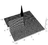
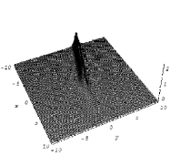
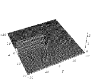
(a)(b)(c)

 

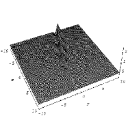
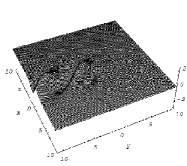
(d)(e)

Figure 1: Single line soliton of eqs.(2), which is obtained by tau-functions of (6). (a) $-L$ , (b) $|S^{(1)}|$, (c) $|S^{(2)}|$, (d) ${\rm Re}\,[S^{(1)}]$, (e) ${\rm Re}\,[S^{(2)}]$. The parameters are $p=1+{\rm i},q=-1+2{\rm i},r=-2+{\rm i}$.

For instance by taking $M=L=1$, (1+1)-soliton solution is given as

$${\cal G}f=c\Big{(}\frac{p+p^{*}}{q+q^{*}}\frac{s+s^{*}}{r+r^{*}}\frac{1}{|p+s^{*}|^{2}}-\frac{s+s^{*}}{r+r^{*}}e^{\xi+\xi^{*}-\eta-\eta^{*}}-\frac{p+p^{*}}{q+q^{*}}e^{\theta+\theta^{*}-\zeta-\zeta^{*}}$$

$$\qquad+|p-s|^{2}e^{\xi+\xi^{*}-\eta-\eta^{*}+\theta+\theta^{*}-\zeta-\zeta^{*}}\Big{)},$$

$${\cal G}g=c(p+p^{*})e^{\xi-\eta}\Big{(}\frac{s+s^{*}}{r+r^{*}}\frac{1}{p^{*}+s}-(p-s)e^{\theta+\theta^{*}-\zeta-\zeta^{*}}\Big{)},$$

$${\cal G}h=-c(s+s^{*})e^{\theta^{*}-\zeta^{*}}\Big{(}\frac{p+p^{*}}{q+q^{*}}\frac{1}{p^{*}+s}+(p^{*}-s^{*})e^{\xi+\xi^{*}-\eta-\eta^{*}}\Big{)},$$

$${\cal G}k=c\frac{(p+p^{*})(s+s^{*})}{p+s^{*}}e^{\xi^{*}-\eta^{*}+\theta-\zeta},$$

where $c=-|(p-s)(p+s^{*})|^{2}$ and we dropped the index 1 for simplicity. In order to satisfy the regularity condition $f\neq 0$, we can take ${\rm Re}\,p>0$, ${\rm Re}\,s>0$, ${\rm Re}\,q<0$ and ${\rm Re}\,r<0$. After removing the gauge and constant factors, by choosing the same wave number in $x$ direction for the above two solitons, i.e., $s=p$, we obtain the single soliton solution,

$$f=\frac{1}{p+p^{*}}-e^{\xi+\xi^{*}}((q+q^{*})e^{-\eta-\eta^{*}}+(r+r^{*})e^{-\zeta-\zeta^{*}}),$$

$$g=(q+q^{*})e^{\xi-\eta},\,h=-(r+r^{*})e^{\xi^{*}-\zeta^{*}},\,k=(q+q^{*})(r+r^{*})e^{\xi+\xi^{*}-\eta^{*}-\zeta},$$ (6)

where $\xi=px-ip^{2}y$, $\eta=q(y-t)+\eta_{0}$ and $\zeta=-r(y+t)+\zeta_{0}$. Figure 1 shows the plots of this single soliton solution. $L$ shows V-shape soliton, $|S^{(1)}|$ and $|S^{(2)}$ shows solitoff behaviour [14].

3 Solutions in the case without $Q$

We consider the 2c-2d-LSRI system (1) without the fourth field $Q$ in (2). This system (1) describes waves in the two-layer fluid. Setting $L=-(2\log F)_{xx},\,S^{(1)}=G/F,\,S^{(2)}=H/F\,,$ we have

$$[{\rm i}(D_{t}+D_{y})-D_{x}^{2}]G\cdot F=0\,,\qquad[{\rm i}(D_{t}-D_{y})-D_{x}^{2}]H\cdot F=0\,,$$

$$-(D_{t}D_{x}-2c)F\cdot F=2GG^{*}+2HH^{*}\,.$$

Here we consider the case of $c=0$.

Using the procedure of the Hirota bilinear method, we obtain the single soliton solution

$$F=1+A_{11}\exp(\eta_{1}+\eta_{1}^{*})\,,\quad G=a_{1}\exp(\eta_{1})\,,\quad H=b_{1}\exp(\xi_{1})\,,$$

$$\eta_{j}=p_{j}x+{\rm i}q_{j}y+\lambda_{j}t+\eta_{j}^{(0)}\,,\qquad\xi_{j}=p_{j}x-{\rm i}q_{j}y+\lambda_{j}t+\eta_{j}^{(0)}\,,\qquad$$

$$A_{11}=-\frac{a_{1}a_{1}^{*}+b_{1}b_{1}^{*}}{(p_{1}+p_{1}^{*})(\lambda_{1}+\lambda_{1}^{*})}\,,\quad\lambda_{1}=-{\rm i}p_{1}^{2}-{\rm i}q_{1}\,.$$

Here $q_{j}$ is a real number. We can rewrite $A_{11}$ as

$$A_{11}=-\frac{a_{1}a_{1}^{*}+b_{1}b_{1}^{*}}{(p_{1}+p_{1}^{*})^{2}({\rm i}p_{1}^{*}-{\rm i}p_{1})}\,.$$

Thus we have

$$S^{(1)}=\frac{a_{1}\exp(\eta_{1})}{1+A_{11}\exp(\eta_{1}+\eta_{1}^{*})}\,,\quad S^{(2)}=\frac{b_{1}\exp(\xi_{1})}{1+A_{11}\exp(\eta_{1}+\eta_{1}^{*})}\,,\quad$$

$$L=-2\frac{\partial^{2}}{\partial x^{2}}\log(1+A_{11}\exp(\eta_{1}+\eta_{1}^{*}))\,.$$

Since $|S^{(1)}|^{2}=GG^{*}/F^{2}$, $|S^{(2)}|^{2}=HH^{*}/F^{2}$, $L=-2\frac{\partial^{2}}{\partial x^{2}}\log F$ do not include $y$, all solitons propagate in the $x$ direction.

There is an exact solution depending on $y$-variable,

$$S^{(1)}=\frac{A_{1}\exp(px+qy+rt)}{1+\exp(2(px+qy+rt))}\exp({\rm i}(k_{1}x+l_{1}y+m_{1}t))\,,\quad$$

$$S^{(2)}=\frac{A_{2}\exp(px+qy+rt)}{1+\exp(2(px+qy+rt))}\exp({\rm i}(k_{2}x+l_{2}y+m_{2}t))\,,\quad$$

$$L=\frac{A\exp(2(px+qy+rt))}{(1+\exp(2(px+qy+rt)))^{2}}\,,$$

where $p$, $q$, $r$, $k_{1}$, $l_{1}$, $m_{1}$, $k_{2}$, $l_{2}$, $m_{2}$, $A_{1}$, $A_{2}$, $A$ satisfy the relations $r=(k_{1}+k_{2})p,\,q=(k_{1}-k_{2})p,\,m_{1}=k_{1}^{2}-l_{1}-p^{2},\,m_{2}=k_{2}^{2}+l_{2}-p^{2},\,A=-8p^{2},\,A_{1}^{2}+A_{2}^{2}=-4(k_{1}+k_{2})p^{2}$, and $p,q,k_{1},l_{1},l_{2}$ are arbitrary parameters.

  

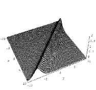
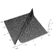
(a)(b)(c)

 

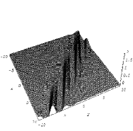
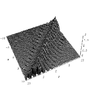
(d)(e)

Figure 2: Line soliton of eqs.(1). (a) $-L$ , (b) $|S^{(1)}|$, (c) $|S^{(2)}|$, (d) ${\rm Re}\,[S^{(1)}]$, (e) ${\rm Re}\,[S^{(2)}]$. The parameters are $k_{1}=-1,k_{2}=-2,A_{1}=1,A_{2}=2,l_{1}=3,l_{2}=4$.

In figure 2, we see that waves in $S^{(1)}$ and $S^{(2)}$ have different modulation property, i.e., carrier waves in $S^{(1)}$ and $S^{(2)}$ has different directions of propagation. Note that the solutions of equations (2) also have this property.

It seems that eqs.(1) are nonintegrable and do not admit general $N$-soliton solution. Similar system (2) has an $N$-soliton solution, but its physical derivation has not been done yet.

4 Concluding Remarks

We have studied solutions of a new integrable two-component two-dimensional long wave-short wave resonant interaction (2c-2d LSRI) system (2). We presented a Wronskian formula for 2c-2d LSRI system (2) with complex conjugacy condition. We have also presented solutions of the system (1) in the case of two-layer fluid, i.e. the 2c-2d LSRI system without $Q$. In this case, the system (1) seems to be non-integrable, i.e. the system (1) does not have multi-soliton solutions. We have found that waves in $S^{(1)}$ and $S^{(2)}$ in both systems have different modulation property, i.e., carrier waves in $S^{(1)}$ and $S^{(2)}$ has different directions of propagation. But the system (2) has much more interesting solutions such as the V-shape soliton and solitoff because of integrability.

One of authors (K. M.) wishes to acknowledge organizers for providing the financial support for the ISLAND 3 (Integrable Systems: Linear And Nonlinear Dynamics 3) conference.

References

[1]
M. J. Ablowitz, B. Prinari and A. D. Trubatch,
Discrete and Continuous Nonlinear Schrödinger Systems,
(Cambridge University Press, 2004).
[2]
S. V. Manakov,
On the theory of two-dimensional stationary self-focusing of electromagnetic waves,
Sov. Phys. JETP 38 (1974), 248–253.
[3]
R. Radhakrishnan, M. Lakshmanan, and J. Hietarinta,
Inelastic collision and switching of coupled bright solitons in optical fibers ,
Phys. Rev. E 56 (1997), 2213–2216.
[4]
M. J. Ablowitz, B. Prinari and A. D. Trubatch,
Soliton interactions in the vector NLS equation,
Inv. Probl. 20 (2004), 1217–1237.
[5]
M. Oikawa, Y. Ohta, K. Maruno, In preparation : Talk at the RIAM
conference 2006, Kyushu University.
[6]
M. Onorato, A. R. Osborne and M. Serio,
Modulational Instability in Crossing Sea States: A Possible
Mechanism for the Formation of Freak Waves,
Phys. Rev. Lett. 96 (2006), 014503-1–014503-4.
[7]
N. Yajima and M. Oikawa,
Formation and interaction of sonic-Langmuir solitons
–inverse scattering method,
Prog. Theor. Phys. 56 (1976), 1719–1739.
[8]
M. Oikawa, M. Okamura and M. Funakoshi,
Two-Dimensional Resonant Interaction between Long and Short Waves,
J. Phys. Soc. Jpn. 58 (1989), 4416–4430.
[9]
Y. Ohta, K. Maruno and M. Oikawa,
Two-component analogue of two-dimensional long wave-short wave resonance interaction equations: a derivation and solutions,
J. Phys.A: Math. Theor. 40 (2007), 7659–7672.
[10]
E. Date, M. Jimbo, M. Kashiwara and T. Miwa,
Transformation groups for soliton equations. III. Operator approach to the Kadomtsev-Petviashvili equation,
J. Phys. Soc. Jpn. 50 (1981), 3806–3812.
[11]
E. Date, M. Jimbo, M. Kashiwara and T. Miwa,
Transformation group for soliton equations: Euclidean Lie algebras
and reduction of the KP hierarchy,
Publ. Res. Inst. Math. Sci. 18 (1982), 1077–1111.
[12]
R. Hirota,
The Direct Method in Soliton Theory,
(Cambridge University Press, 2004).
[13]
J. Hietarinta and R. Hirota,
Multidromion solutions to the Davey-Stewartson equation,
Phys. Lett. A 145 (1990), 237–244.
[14]
C.R. Gilson, Resonant behaviour in the Davey-Stewartson equation,
Phys. Lett. A 161 (1992), 423–428.