Detecting barrier to cross-jet Lagrangian transport and its destruction in a meandering flow

Abstract

Cross-jet transport of passive scalars in a kinematic model of the meandering laminar two-dimensional incompressible flow which is known to produce chaotic mixing is studied. We develop a method for detecting barriers to cross-jet transport in the phase space which is a physical space for our model. Using tools from theory of nontwist maps, we construct a central invariant curve and compute its characteristics that may serve good indicators of the existence of a central transport barrier, its strength, and topology. Computing fractal dimension, length, and winding number of that curve in the parameter space, we study in detail change of its geometry and its destruction that are caused by local bifurcations and a global bifurcation known as reconnection of separatrices of resonances. Scenarios of reconnection are different for odd and even resonances. The central invariant curves with rational and irrational (noble) values of winding numbers are arranged into hierarchical series which are described in terms of continued fractions. Destruction of central transport barrier is illustrated for two ways in the parameter space: when moving along resonant bifurcation curves with rational values of the winding number and along curves with noble (irrational) values.

I Introduction

A meandering jet is a fundamental structure in laboratory and geophysical fluid flows. Strong oceanic and atmospheric jet currents separate water and air masses with distinct physical properties. For example, the Gulf Stream separates the colder and fresher slope ocean waters from the salty and warmer Sargasso sea ones. Recently, there has been much interest in applying ideas and methods from dynamical systems theory to study mixing and transport in meandering jets. In steady horizontal velocity fields, water (air) parcels move along streamlines in a regular way. When the velocity field changes in time, the motion becomes much more complicated even if the change is periodic. The phenomenon of chaotic advection of passive particles in (quasi)periodically-disturbed fluid flows has been studied theoretically and experimentally A65 ; A84 ; A02 ; Ottino .

In the context of dynamical systems theory, chaotic advection is Hamiltonian chaos in two-dimensional incompressible flows (for a review of Hamiltonian chaos see, for example, AKN85 ; LL84 ; Ott ; Z05 ). The coordinates $x$ and $y$ of a passive particle on the horizontal plane satisfy to simple Lagrangian equations of motion

$$\frac{dx}{dt}=u(x,y,t)=-\frac{\partial\Psi}{\partial y},\quad\frac{dy}{dt}=v(x,y,t)=\frac{\partial\Psi}{\partial x},$$ (1)

where $u$ and $v$ are zonal and meridional velocities of the particle, and the stream function $\Psi$ plays the role of a Hamiltonian. The phase space of the dynamical system (1) with one and half degrees of freedom is a configuration space for passive particles.

A number of simple kinematic and dynamically consistent model stream functions have been proposed to study large-scale chaotic mixing and transport in geophysical meandering jet flows S92 ; DW96 ; Miller97 ; YPJ02 ; Chaos06 ; UlBP07 ; PK06 ; Book08 . Deterministic models do not pretend to quantify transport fluxes in real oceanic and atmospheric currents but they are useful to reveal large-scale space-time structures that specify qualitatively mixing and transport of water and air masses. Whether or not the jet provides an effective barrier to meridional or cross-jet transport, under which conditions the barrier becomes permeable and to which extent, these are crucial questions in physical oceanography and physics of the atmosphere. The problem must be treated from different points of view. In the straightforward numerical approach based on full-physics nonlinear models, the velocity field is generated as an outcome of a basin circulation model and a flux across the jet (if any) can be estimated integrating a large number of tracers. The kinematic and linear dynamically consistent models are less realistic, but they allows to identify and analyze different factors which could enhance or suppress the cross-barrier transport.

As to meandering currents, both the approaches have been applied to study cross-jet Lagrangian transport. A simple kinematic model with the basic streamfunction in the form (2) has been shown to reproduce some features of the large-scale Lagrangian dynamics of the Gulf Stream water masses B89 . The phase portrait of Eqs. (1) with the meandering Bickley jet (2) is plotted in Fig. 1 (a) in the frame moving with the meander phase velocity. Time dependence of the meander amplitude or the introduction of a secondary meander, superimposed on the basic flow, may break the boundaries between distinct regions in Fig. 1 (a) producing chaotic mixing and transport between them S92 ; Meyers94 ; DW96 ; Chaos06 ; UlBP07 ; JPA08 . The numerical calculations, based on computing the Melnikov function Melnik , have shown that transport across the jet was much weaker than that between the jet ($J$), the circulation cells ($C$), and the peripheral currents ($P$) in Fig. 1 (a), i. e. the perturbation mixes the water along each side of the jet more efficiently than across the jet core S92 . An attempt to analytically predict the parameter values for the destruction of the transport barrier was made in Ref. Meyers94 using the heuristic Chirikov criterion for overlapping resonances Chir79 . A technique, based on computing the finite-scale Lyapunov exponent, as a function of initial position of tracers, has been found useful in Ref. BLR01 to detect the presence of cross-jet barriers in the kinematic model (2). An analysis of cross-jet transport, based on lobe dynamics, has been applied in RWig06 to describe how particles can cross the jet from the north to the south and vice versa.

The study of cross-jet transport has been motivated also by a series of laboratory experiments SMS89 ; BMS91 ; SHS93 on Rossby waves propagating along an azimuthal jet in a rapidly rotating tank. This flow can be modeled in the linear approximation of the corresponding fluid equations DM93 by a stream function which is a superposition of a Bickley jet and two neutral modes (Rossby waves). The destruction of a barrier to cross-jet transport has been studied analytically by using the Chirikov criterion in the pendulum approximation and numerically by using Poincaré sections DM93 . It was shown that one needs very large values of the perturbation amplitudes to break the barrier. The analytic model proposed in DM93 has been used recently to study Lagrangian dynamics of atmospheric zonal jets and the permeability of the stratospheric polar vortex. Poincaré sections and finite-time Lyapunov exponents revealed a robust transport barrier which can be broken either due to large perturbation amplitudes of the Rossby waves or as a result of an increase of their phase velocities Rypina . A comparison of properties of cross-jet transport in ad hoc kinematic and dynamically consistent models of atmospheric zonal jets has been done recently in Ref. P.H.Haynes .

Being motivated by Lagrangian observations of the oceanic currents, cross-jet transport and mixing have been studied in numerical models of meandering jets Miller97 ; YPJ02 ; YPJ04 . It has been shown both in barotropic and baroclinic nonlinear numerical models, where the meander amplitude can not be made arbitrary large, that cross-jet chaotic transport, resulting from the meandering motions, are maximized at a subsurface level. Since the undisturbed velocity is weaker at deeper levels, the corresponding separatrices are closer to the jet core. Therefore, separatrix reconnection should occur below some critical depth and transport across the jet should be facilitated.

Independent on the work on cross-jet transport in the geophysical community, there have been a number of theoretical and numerical investigations of chaotic transport in so-called area-preserving nontwist maps HH84 ; W88 ; DM93 ; PhysD96 ; Aizawa ; PhysD97 ; Shinohara97 ; Wurm05 ; Wurm04 . We mention specially the early study of different reconnection scenario HH84 ; W88 and the first systematic study of cross-jet transport in nontwist maps DM93 ; PhysD96 ; PhysD97 . These maps locally violate the twist condition, a map analogue of the non-degeneracy condition for Hamiltonian systems. Nontwist maps are of interest because many important mathematical results, including KAM and Aubry-Mather theory, depend on the twist condition. Apart from their mathematical importance, nontwist maps are of a physical interest because they are able to model transition to global chaos, the term meaning in the mathematical community a cross-jet transport. Nontwist maps allow to study different scenarios for this transition: reconnection of separatrices, meandering and breakup of invariant tori, and others.

The onset of global chaos in oscillatory Hamiltonian systems, where the eigenfrequency possesses a local extremum as a function of energy, has been studied analytically and numerically in Refs. SMSoskin ; S.M.S . In such systems with two or more separatrices, global chaos may occur at unusually small magnitudes of perturbation due to overlap in the phase space between resonances of the same order and their overlap in energy with chaotic layers of the corresponding unperturbed separatrices.

In the present paper we develop a method for detecting a barrier to cross-jet Lagrangian transport (or global chaos in a more general context), apply it to the kinematic model of a meandering jet flow, study changes in its topology under varying the perturbation parameters, and scenarios of its destruction. In Sec. II we briefly introduce a model streamfunction which is known to produce chaotic advection S92 ; Chaos06 ; RWig06 and compute the amplitude–frequency $\varepsilon$–$\nu$ diagram demonstrating the parameter range for which cross-jet transport exists. Based on the symmetry of the flow, we propose in Sec. IIIa a numerical method to identify a central invariant curve (CIC) which is a diagnostic means to detect the process of destruction of a central transport barrier (CTB). The CIC is constructed by successive iterations of so-called indicator points Aizawa . Computing the fractal dimension of a set of iterations of those points at different values of the parameters, we identify whether the CIC and CTB are broken or not. In Sec. IIIb we study possible geometries of the CIC that may change dramatically with varying $\varepsilon$ and $\nu$. Before the total destruction, the CIC experiences a number of local bifurcations becoming a complicated meandering curve whose properties can be specified by its length and the winding number $w$. A structure of the set of CICs is revealed in a continued fraction representation of their winding numbers. The CICs with rational $w$ are arranged in hierarchical series connected with the corresponding resonances. Whereas, the CICs with noble numbers form their own series. Destruction of CTB is studied in Sec. IV for two ways in the parameter space. When moving along a so-called resonant bifurcation curve with a rational value of $w$, one specifies the values of $\varepsilon$ and $\nu$ for which the CIC is broken but CTB remains. In contrary to that, when moving along any curve with noble value of $w$, a CIC exists providing CTB. The process of CTB destruction in both the cases is illustrated in Sec. IV.

II The amplitude–frequency diagram for cross-jet transport in the model flow

We take the Bickley jet with a running wave imposed as a kinematic model of a meandering shear flow in the ocean. The respective normalized stream function in the frame moving with the phase velocity of the meander has the following form Chaos06 :

$$\Psi=-\tanh{\left(\frac{y-A\cos x}{L_{\text{jet}}\sqrt{1+A^{2}\sin^{2}x}}\right)}+Cy,$$ (2)

where the jet’s width $L_{\text{jet}}$, meander’s amplitude $A$ and its phase velocity $C$ are the control parameters. The phase portrait of the advection equations (1) with the streamfunction (2), shown in Fig. 1 (a), consists of three different regions: the central eastward jet $J$, chains of the northern and southern circulation cells $C$ and the peripheral westward currents $P$. The flow is steady in the moving frame of reference, and passive particles follow the streamlines. In Fig. 1 (b) we plot a frequency map $f(x_{0},y_{0})$ that shows by nuances of the grey color the value of the frequency $f$ of particles with initial positions ($x_{0},y_{0}$) in the unperturbed system. The maximal value of the frequency, $f_{\text{max}}=1.278$, have the particles moving in the central jet.

As a perturbation, we take the simple periodic modulation of the meander’s amplitude

$$A=A_{0}+\varepsilon\cos\nu t.$$ (3)

Under the perturbation, the separatrices, connecting saddle points, are destroyed and transformed into stochastic layers. The strength of chaos depends strongly on both the perturbation parameters, the perturbation amplitude $\varepsilon$ and frequency $\nu$. In the model used the normalized control parameters are connected with the dimensional ones as follows Chaos06 : $A=ak$, $C=c/u_{\text{m}}\lambda k$, and $L_{\text{jet}}=\lambda k$, where $a,k$, and $c$ are amplitude, wave number, and phase velocity of a meander, respectively, $\lambda$ and $u_{\text{m}}$ are characteristic width and maximal zonal velocity in the jet on the surface. All these parameters change in a wide range in the Gulf Stream B89 ; S92 ; Meyers94 : $\lambda\simeq 40\div 100$ km, $a\simeq 50\div 60$ km, $2\pi/k\simeq 200\div 400$ km, $c\simeq 0.1\div 0.5$ m/sec, $u_{\text{m}}\simeq 1\div 1.5$ m/sec. So, we get $L_{\text{jet}}\simeq 0.1\div 3$, $A\simeq 0.7\div 2$, and $C\simeq 0.02\div 0.3$. Being motivated by mixing and transport in the Gulf Stream, we took the following normalized values of the control parameters that will be used in all our numerical experiments: $A_{0}=0.785,C=0.1168$ and $L_{\text{jet}}=0.628$.

The equations of motion (1) with the stream function (2) and the perturbation (3) have the symmetry

$$\hat{S}:\left\{\begin{aligned} x^{\prime}&=\pi+x,\\ y^{\prime}&=-y\end{aligned}\right.$$ (4)

and the time reversal symmetry

$$\hat{I}_{0}:\left\{\begin{aligned} x^{\prime}&=-x,\\ y^{\prime}&=y.\end{aligned}\right.$$ (5)

The symmetries (4) and (5) are involutions, i. e. $\hat{S}^{2}=1$ and $\hat{I}_{0}^{2}=1$. Due to the symmetry $\hat{S}$, motion can be considered on the cylinder with $0\leq x\leq 2\pi$. The part of the phase space with $2\pi n\leq x\leq 2\pi(n+1)$, $n=0,\pm 1,\dots$, is called a frame. It should be stressed that the phase space in two-dimensional incompressible flows is a configuration space for advected particles.

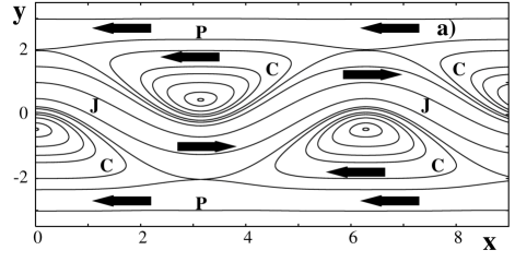
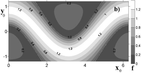
Figure 1: (a) Phase portrait of the unperturbed flow in the frame moving with the meander’s phase velocity. Streamlines in the circulation cells ($C$), jet ($J$), and peripheral currents ($P$) are shown. (b) Frequency map represents by color values of the frequency $f$ of particles with initial positions ($x_{0},y_{0}$) advected by the unperturbed flow.

The following numerical procedure has been applied to establish the fact of cross-jet transport in the kinematic model of the meandering jet current. The advection equations (1) for given values of the perturbation amplitude $\varepsilon$ and frequency $\nu$ and with twenty particles, released nearby the northern saddle point, have been integrated up to the time instant when one of the particles was detected to cross the straight line $y=y_{s}$ passing through the southern saddle. If after the time $T_{\text{max}}=1000\times 2\pi/\nu$ none of the particles crosses the line $y=y_{s}$, we assume that for given values of the parameters there is no cross-jet transport. The $\varepsilon$–$\nu$ diagram in Fig. 2 shows the values of the parameters for which cross-jet chaotic transport exists (white-color zones). There are a number of the frequency values for which transport occurs at surprisingly small values of the perturbation amplitude $\varepsilon$. The absolute minimal value of the perturbation amplitude, at which the cross-jet chaotic transport occurs, $\varepsilon_{\text{min}}=0.0218\approx A_{0}/36$, corresponds to the frequency $\nu=1.165$ which is close to the natural frequencies of the particles moving in the central jet.

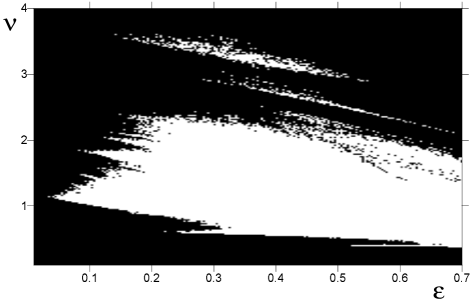
Figure 2: Amplitude–frequency $\varepsilon$–$\nu$ diagram showing the parameter values for which cross-jet chaotic transport exists (white zones) or not (black zones).

III Topology of a barrier to cross-jet transport and central invariant curve

The amplitude–frequency diagram is useful to detect cross-jet transport but its computation is a time consuming procedure. Moreover, it says nothing about the properties of barrier to transport and mechanism of its destruction. A fractal-like boundary between the colors in Fig. 2 reflects an intermittency in appearance and destruction of the cross-jet barrier when varying $\varepsilon$ and $\nu$. Further insight into topology of the barrier could be obtained if one would be able to find an indicator of cross-jet transport, i. e. an object in the phase space whose form contains an information about permeability of the barrier.

III.1 Detecting the central invariant curve

First of all, we need to give definitions of some basic structures specifying a cross-jet barrier and its destruction. The central transport barrier (CTB) is defined as a strip between the southern and northern unperturbed separatrices confined by marginal northern and southern ballistic trajectories (excluding orbits of ballistic resonances in the stochastic layer). All the trajectories inside the CTB are ballistic, some of them are regular and the other ones are chaotic. The amplitude–frequency diagram in Fig. 2 demonstrates clearly destruction of the CTB at some values of the perturbation parameters $\varepsilon$ and $\nu$ and onset of cross-jet transport.

Our Hamiltonian flow with the streamfunction (2) is degenerate, i. e. it violates the non-degeneracy condition, $\partial f/\partial I\neq 0$, for some values of the natural frequency of passive particles $f$ and their actions $I$ in the unperturbed system. Physically it means that the zonal velocity profile $u(y)$ has a maximum. In theory of nontwist maps the curve, for which the twist condition (analogue of the non-degeneracy condition) is violated, is called a nonmonotonic curve Wurm05 . In our model flow (2) it is some value of unperturbed streamfunction along which the frequency $f$ is maximal (see Fig. 1 (b)).

Instead of integrating the advection equations (1), we integrate the corresponding Poincaré map, an orbit of which is defined as a set of points $\{(x_{i},y_{i})\}_{i=-\infty}^{\infty}$ on the phase plane such that $\hat{G}_{T}(x_{i},y_{i})=(x_{i+1},y_{i+1})$, where $\hat{G}_{t}$ is an evolution operator on a time interval $t$ and $T\equiv 2\pi/\nu$ is the period of perturbation. Operator $\hat{G}_{T}$ can be factorized as a product of two involutions $\hat{G}_{T}=\hat{I}_{1}\hat{I}_{0}$, where $\hat{I}_{1}=\hat{G}_{T}\hat{I}_{0}$  is also a time reversal simmetry PhysD96 .

A periodic orbit of period $nT$ ($n=1,2,\dots$) is an orbit such that $(x_{i+n},y_{i+n})=(x_{i}+2\pi m,y_{i})$, $\forall i$, where $m$ is an integer. An invariant curve is a curve invariant under the map. The nonmonotonic curve is not an invariant curve under a perturbation. The winding (or rotation) number $w$ of an orbit is defined as the limit $w=\lim\limits_{i\to\infty}[(x_{i}-x_{0})/(2\pi i)]$, when it exists. The winding number is a ratio between the frequency of perturbation $\nu$ and the natural frequency $f$. Periodic orbits have rational winding numbers $w=m/n$. It simply means that a ballistic passive particle in the flow flies $m$ frames before returning to its initial position $x_{0}$ (modulo $2\pi$) after $n$ periods of perturbation. Winding numbers of quasiperiodic orbits are irrational.

Now we are ready to introduce the important notion of a central invariant curve (CIC). We define CIC as an curve which is invariant under the operators $\hat{S}$ and $\hat{G}_{T}$. It can be shown, that two curves invariant under $\hat{S}$ have at least two common points. The curves, which are invariant under $\hat{G}_{T}$, cannot intersect each other. So, the CIC is a unique curve. Following to Ref. Shinohara97 , one can show that the CIC corresponds to a local extremum on the winding number profile with an irrational value of $w$. Such curves are called <<shearless curves>> in theory of nontwist maps Wurm05 . The significance of a shearless curve is that it acts as a barrier to global transport in the phase space of a nontwist map. The violation of the twist condition leads to existence of more than one orbit with the same winding number arising in pairs on both sides of the shearless curve. Those pairs of orbits can collide and annihilate at certain parameter values. The collision of the orbits involves in phenomenon, which was called as reconnection of invariant manifolds of the corresponding hyperbolic orbits HH84 .

The CIC should not be thought as the last cross-jet barrier curve in the CTB in the sense that it breaks down under increasing the perturbation amplitude in the last turn. Sometimes it is the case, but sometimes it is not. Nevertheless, the CIC serves a good indicator of the strength of the CTB and its topology.

The CIC can be constructed by successive iterations of so-called indicator points Aizawa . In our model flow (2) with the symmetries (4) and (5), indicator points are the points ($x_{j}^{(k)}$, $y_{j}^{(k)}$), $k=1,2$, which are solutions of the equations

$$\hat{I}_{0}(x_{j}^{(1)},y_{j}^{(1)})=\hat{S}(x_{j}^{(1)},y_{j}^{(1)}),$$ (6)

or

$$\hat{I}_{1}(x_{j}^{(2)},y_{j}^{(2)})=\hat{S}(x_{j}^{(2)},y_{j}^{(2)}),$$ (7)

where index $j$ numerates the points. The equation (6) gives a pair of indicator points: ($x_{1}^{(1)}=\pi/2$, $y_{1}^{(1)}=0$) and ($x_{2}^{(1)}=3\pi/2$, $y_{2}^{(1)}=0$). Instead of solving Eq. (7) we solve the equivalent equation

$$\hat{G}_{T}(x,y)=\hat{I}_{0}\hat{S}(x,y)\equiv(\pi-x,-y).$$ (8)

If some ($x$, $y$) is a solution of (8), then $\hat{I}_{0}(x$, $y)$  is a solution of (7). The equation (8) cannot be solved analitically, so we apply the numerical method based on computing a minimum of the function $r(x,y)=||\hat{G}_{T}(x,y)-(\pi-x,-y)||$, where $||\cdot||$ is a norm on the cylinder. Since $r(x,y)\geq 0$ for any $(x,y)$, the points with $r(x,y)=0$ are minima of the function $r(x,y)$. Thus, solution of Eq. (8) reduces to searching for a local minimum of the function $r(x,y)$ with the additional condition $r(x,y)=0$ at the point of the minimum. There are a number of numerical methods for doing that job. We prefer to use the downhill simplex method. In our problem the function $r(x,y)$ always has two minima, i. e. two indicator points transforming to each other under action of the operator $\hat{S}$.

Next, we study iterations, i. e. Poincaré mapping of one of the indicator points $(x_{0},y_{0})$. If the iterations $(x_{i},y_{i})=\hat{G}_{T}^{i}(x_{0},y_{0})$ are confined between invariant curves in a bounded region, the following three cases are possible in dependence on the dimension $d$ of the set $(x_{i},y_{i})$:

1) The iterations lie on a curve on the phase plane with $d=1$ which is a CIC.

2) The iterations is an organized set of points with $d=0$. It means that they constitute either a central periodic orbit or a central almost periodic orbit, an orbit that could not form a smooth curve on the phase plane for a limited integration time.

3) The iterations form a central stochastic layer with $d=2$.

If the iterations are not confined by any invariant curves in a bounded region, i. e. they occupy all the accessible phase plane to the south and north from the central jet, then there exists global chaotic transport. Thus, the type of motion of indicator points provides an indicator of global chaos and the absence of barriers to cross-jet transport.

Possible topologies of the corresponding CTB at the fixed frequency $\nu=1.2$ and with increasing values of the perturbation amplitude $\varepsilon$ are illustrated in Fig. 3 plotting iterations of the indicator points computed by the above-mentioned method. The panel (a) illustrates the case when those iterations form a CIC. Another typical situation is shown in Fig. 3 (b) where the iterations fall in small segments filling at $\tau\to\infty$ a continuous curve which is a central almost periodic orbit. If the iterations fill up not a curve but a bounded region between invariant curves, then there appears a central stochastic layer preventing cross-jet transport (Fig. 3 (c)). When iterations of the indicator points occupy a region that is not confined by any invariant curves, it means destruction of the CTB and onset of global chaos, i. e., chaos in a large region of the phase space accompanied by cross-jet transport.

The indicator points have been found with the help of the above-mentioned numerical procedure, and their iterations have been computed in the following range of the control parameters: $\nu\in[0.95:1.5]$ and $\varepsilon\in[0.01:1]$. We assume that the iterations are bounded, if their coordinates do not cross the unperturbed separatrices after $5\times 10^{4}$ iterations. The dimension $d$ of the set of those iterations is computed by the box-counting method, where the value of $d$ for the box size $e_{k}=(1/2)^{k}$ is defined as

$$d_{k}=\log_{2}\frac{N_{k+1}}{N_{k}},$$ (9)

where $N_{k}$ is a number of boxes of the size $e_{k}$ containing set points. The dimension $d_{k}$ goes to zero with decreasing $e_{k}$, and one cannot distinguish in this limit between the central almost periodic orbit and the central stochastic layer at large $k$. Comparing the values of $d_{k}$ at different values of $k$, we were able to find the empirical value $k=4$ which is enough to make the difference.

The results of computation of the dimension $d_{4}(\varepsilon,\nu)$ for a set of iterations of the indicator points are shown in the bird-wing diagram in Fig. 4. That one and the other bird-wing diagrams in the parameter space show the properties of CTB and CIC in the range of comparatively small values of the perturbation amplitude ($0.01\leq\varepsilon\leq 0.1$) and the frequency ($1.15\leq\nu\leq 1.5$) corresponding to particles moving in the central jet (Fig. 1 (b)). White color corresponds to the regime of global chaotic transport with unbounded motion of iterations of the indicator points. Otherwise, the CTB exists but its topology is different. Grey color means that there exists a CIC with $0.95\leq d_{4}\leq 1.05$ in the corresponding range of the parameters. White rectangles, which are hardly visible in the main panel (see their magnification on the inset of the figure), means existence of a central almost periodic orbit with $d_{4}<0.95$ and black strips — a central stochastic layer with $d_{4}>1.05$.

III.2 Geometry of the central invariant curve and its bifurcations

To quantify complexity of the CIC we define its length $L$ as a sum of the distances between the iterations of the indicator points $(x_{i},y_{i})$ ordered on the phase plane in the following way:

1. The first step. A point $B_{0}$, belonging to a set of iterations of the Poincaré map $(x_{i},y_{i})$, is marked.

2. The $(j+1)$-th step. We find and mark among all the unmarked points that one, $B_{j+1}$, which minimizes the Euclidean distance $D_{j}=D(B_{j},B_{j+1})$ between $B_{j}$ and $B_{j+1}$.

3. The procedure is repeated unless all the points will be marked.

Figure 3: Poincaré mapping of indicator points. In the first three panels the orbit of these points is bounded and there exists a central transport barrier (CTB) with (a) CIC $(\varepsilon=0.01,\nu=1.2)$, (b) central almost periodic orbit $(\varepsilon=0.011997277,\nu=1.2)$, and (c) central stochastic layer at $(\varepsilon=0.01177,\nu=1.2)$ with the inset demonstrating a magnification of a small region. (d) Destruction of CTB and onset of global chaotic transport as a result of unbounded iterations of indicator points $(\varepsilon=0.041,\nu=1.2)$.

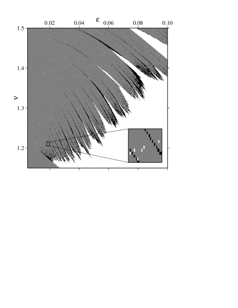
Figure 4: Bird-wing diagram of the box-counting dimension $d_{4}(\varepsilon,\nu)$. White color: regime with global chaotic transport with unbounded motion of indicator points (see Fig. 3 (d)). If the motion of indicator points is bounded, then there exists a CTB but its topology may differ. Grey color ($0.95\leq d_{4}\leq 1.05$): regime with a CIC (see Fig. 3 (a)). Small white regions which are hardly visible inside the grey ‘‘wing’’ ($d_{4}<0.95$): regime with a central almost periodic orbit (see Fig. 3 (b)). Black color ($d_{4}>1.05$): regime with a central stochastic layer (see Fig. 3 (c)). Inset shows magnification of a small region in the parameter space with visible white and black regions.

As an output we have an ordered set of points $B_{j}$ constituting a CIC. The accuracy is controlled by the quantity $\max{D_{j}}$. Large values of this quantity mean that the points are ordered in a wrong way or a set of points is chaotic. To increase the number of points we use in addition to the original points $(x_{i},y_{i})$ their ‘‘images’’ $(x_{i}+\pi,-y_{i})$ as well. To minimize the computation time the points are sorted in accordance with their $x$ coordinates.

Figure 5 illustrates metamorphosis of the CIC as the perturbation amplitude increases. We start with the CIC, shown in Fig. 5 (a), which we call a nonmeandering CIC. At the critical value $\varepsilon\approx 0.011758$, invariant manifolds of hyperbolic orbits of two chains of the 1:1 resonance islands on both sides of the CIC connect, and after that the CIC becomes a meandering curve of the first order (Fig. 5 (b)) and period $T$. The period of CIC’s meandering is simply a period of nearby main islands Shinohara97 ; Simo98 . At the next critical value $\varepsilon=0.01178721$, reconnection of invariant manifolds of secondary resonance islands takes place. The corresponding second-order meandering CIC with period $79T$ is shown in Fig. 5 (c). Highly meandering CICs of higher orders appear with further increasing the perturbation amplitude (Fig. 5 (d)).

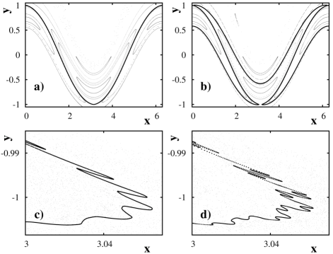
Figure 5: Metamorphosis of the central invariant curve (CIC). (a) Nonmeandering CIC ($\nu=1.2$, $\varepsilon=0.01174929$). (b) Meandering CIC of the first order and period $T$ ($\nu=1.2$, $\varepsilon=0.01178721$). (c) Meandering CIC of the second order and period $79T$ ($\nu=1.2$, $\varepsilon=0.01179027$). (d) Meandering CIC of a higher order ($\nu=1.2$, $\varepsilon=0.01179339$).

Some smooth invariant curves inside the CTB break down under the perturbation (3), and chains of ballistic resonance islands appear at their place. Those islands appear in pairs to the north and south from a CIC due to the flow symmetries (4) and (5) (see Fig. 5 (a) and (b)). Geometry of the CIC, size and number of the islands, and topology of their invariant manifolds change with variation of the perturbation amplitude $\varepsilon$ and frequency $\nu$ in a very complicated way.

In Fig. 6 we plot in the parameter space the values of the CIC length $L$ coding it by nuances of the grey color. White color corresponds to those values of the parameters $\varepsilon$ and $\nu$ for which cross-jet transport exists due to destruction of the CTB. Black color codes the regime with a broken CIC but a remaining CTB that prevents cross-jet transport ($d_{4}>1.05$). Dotted and dashed lines on the plot are the resonant bifurcation curves along which the CIC winding number $w$ is rational. The $m/n$ resonant bifurcation curve is the set of values of the control parameters for which a reconnection of invariant manifolds of the $n:m$ resonances takes place. The dotted lines correspond to even resonances with $w=~{}(2k~{}-~{}1)~{}/~{}2k$ and the dashed lines are odd resonances with $w=2k/(2k+1)$, $k=1,2,\dots$. All those curves end up in the dips of the bird-wing diagram.

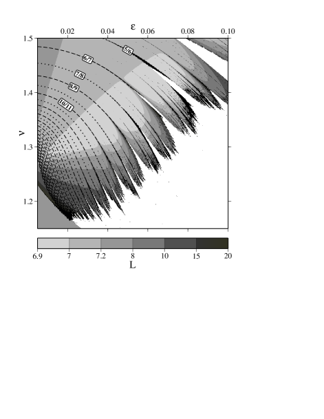
Figure 6: Bird-wing diagram showing the length $L$ of the CIC by nuances of the grey color in the parameter space $(\varepsilon,\nu)$. White zone: regime with a broken CTB and cross-jet transport. Black color: regime with a broken CIC but a remaining CTB preventing cross-jet transport. Resonant bifurcation curves, along which the CIC winding numbers $w$ are rational, end up in the dips of ‘‘the wing’’. Dotted and dashed lines correspond to even and odd resonances, respectively.

Figure 7: Dependence of the length of CIC $L$ on the perturbation amplitude at the fixed frequency $\nu=1.2$. (a) General view of the dependence $L(\varepsilon)$ in the range of interest $\varepsilon=[0.01175:0.012]$. Vertical dotted lines correspond to rational values of the CIC winding number $w$. The resonance $1/1$ appears at $\varepsilon=0.11756$. The arrangement of the spikes is explained in the text. (b) Magnification of one of the wide spikes in panel (a). Solid line is a winding number profile $w(\varepsilon)$ with the value $w=62/63$ shown by the dashed line.

In order to analyze a fractal-like boundary of the bird-wing diagram in Fig. 6, we cross it horizontally at the frequency $\nu=1.2$ and consider the plot $L(\varepsilon)$ in the range of interest of $\varepsilon$ (Fig. 7 (a)). The perturbation frequency $\nu=1.2$ is close to the maximal frequency $f_{\text{max}}$ of particles in the middle of the jet in the unperturbed flow (see Fig. 1 (b)). The plot $L(\varepsilon)$ consists of a number of spikes with different height and width. In the range of small values of the perturbation amplitude ($\varepsilon<0.011756$), the length of the CIC is approximately the same $L\approx 7.35$ (a small fragment of the function $L(\varepsilon)$ is shown in Fig. 7 (a) just to the left from the vertical line $1/1$). In that range, the CIC is a nonmeandering curve (see Fig. 5 (a)) surrounded by smooth invariant curves and $1:1$ resonance islands with a heteroclinic topology. The size of those islands is comparable with the frame size. The width of the CTB, filled by invariant curves around the CIC, decreases with increasing the perturbation amplitude $\varepsilon$.

Figure 8: Poincaré sections at $\nu=1.2$ and increasing values of $\varepsilon$ in the range corresponding to the wide spike with $w=62/63$ in Fig. 7 (b). (a) Meandering CIC surrounded by meandering invariant curves $(\varepsilon=0.011931)$. (b) CIC meandering between the odd $63:62$ islands born as a result of a saddle-center bifurcation ($\varepsilon_{\text{sc}}=0.011934)$. (c) CIC destruction due to connection of invariant manifolds of the $63:62$ islands $(\varepsilon=0.01193511)$. A narrow stochastic layer appears at the place of the CIC. (d) CIC appears again $(\varepsilon=0.0119352)$.

The CIC winding number $w$ changes under a variation of the perturbation amplitude. At $\varepsilon\simeq 0.011756$, invariant manifolds of the 1:1 resonance connect, and a central stochastic layer appears at the place of the CIC. This layer exists up to $\varepsilon\simeq 0.011785$ (see a random set of points in Fig. 7 (a) in that range of $\varepsilon$). At $\varepsilon>0.011785$, the CIC appears again. Now it is a meandering curve of the first order (see Fig. 5 (b)) whose length is larger due to reconnection of the 1:1 resonance islands. As $\varepsilon$ increases further, the CIC length $L$ changes in a wide range. Smooth fragments with approximately the same value of $L\approx 20$ alternate with spikes of different height and width. The spikes are condensed, when approaching to the value $w=1/1$, and overlap in the range $\varepsilon\simeq[0.011756:0.011785]$.

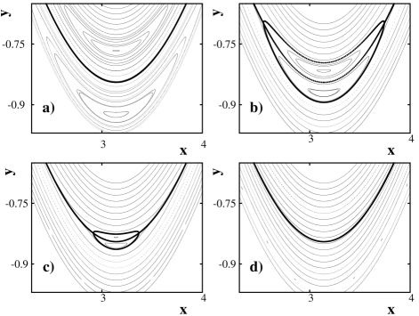
Figure 9: Poincaré sections at $\varepsilon=0.015$ and increasing values of $\nu$. (a) CIC between islands of the even 2:1 resonance ($\nu=2.51<2f_{\text{max}}=2.556$). (b) Reconnection of invariant manifolds of that resonance and a formation of a vortex pair with a narrow stochastic layer shown by bold curves ($\nu=2.55$). (c) The vortex size decreases with increasing $\nu$ ($\nu=2.555$). (d) Past some critical value of $\nu$, the vortex pair disappears and CIC appears again ($\nu=2.56$).

The arrangement of the spikes in Fig. 7 (a) can be explained using a representation of rational numbers by continued fractions. A continued fraction is the expression

$$c=[a_{0};a_{1},a_{2},a_{3},\dots]=a_{0}+\frac{1}{a_{1}+\dfrac{1}{a_{2}+\dfrac{1}{a_{3}+\cdots}}},$$ (10)

where $a_{0}$ is an integer number and the other $a_{n}$ are natural numbers. Any rational (irrational) number can be represented by a continued fraction with a finite (infinite) number of elements. The spikes in Fig. 7 (a) are arranged in convergent series in such a way that each spike in a series generates a series of spikes of the next order. For example, the series of the integer $n:1$ resonance has the winding numbers equal to $1/n$ or $[0;n]$ in the continued-fraction representation. Each spike in that series generates a series of resonance spikes of the next order converging to the parent spike. Winding numbers of those resonances are $[0;n,i]$, $i=2,3,4\dots$ (at $i=1$, one gets a spike in the main series because of the identity $[a_{0};a_{1},\dots,a_{n},1]\equiv[a_{0};a_{1},\dots,a_{n}+1]$). The spikes with $[0;1,i]=i/(i+1)$ converge to the spike of the $1:1$ resonance. That is clearly seen in Fig. 7 (a). The direction of convergence of the spikes in a series alternate with the series order: the winding number increases in the series of the first order, decreases in the series of the second order, and increases again in the series of the third order. That is why a chaotic region in Fig. 7 (a) is situated to the right from the $1:1$ resonance, i. e. in the range of smaller values of $w$. Whereas, it is to the left for the series of the second order, i. e. in the range of larger values of $w$. There also exists an additional hierarchical structure with fractional $1:n$ resonances, whose frequencies are below the $1:1$ resonance frequency, and a series with resonances corresponding to the spikes below $[0;1,i,(1)]$, for example, a clearly visible series of spikes below $[0;1,4,(1)]$ converging to the spike $5/6$ in the $L$ diagram (see Fig. 6).

Unfortunately, we could not identify series of the third and a higher order because numerical errors in identifying the winding numbers are greater than the distance between the spikes of higher-order series. Unresolved regions on the plot $L(\varepsilon)$ in Fig. 7 (a) appear because of a decrease of the distance between the spikes in the same series with increasing series number, a process resembling Chirikov’s overlapping of resonances.

A magnification of one of the wide spikes is shown in Fig. 7 (b). We plot the winding number profile $w(\varepsilon)$ together with the function $L(\varepsilon)$ for the spike. To illustrate what happens with the CIC and its surrounding with increasing $\varepsilon$ we plot the corresponding Poincaré section in Fig. 8. In the range $\varepsilon\simeq[0.0119:0.01192]$ the lengths of the CIC and surrounding invariant curves increase slowly due to small changes in their geometry (Fig. 8 (a)). After a saddle-center bifurcation at $\varepsilon_{\text{sc}}\simeq 0.011934$, there appear two chains of homoclinically connected $63:62$ islands separated by a meandering CIC (Fig. 8 (b)). The amplitude of the CIC meanders increases with further increasing $\varepsilon$ in the range $\varepsilon\simeq[0.011934:0.011935]$. In that range the CIC disappears and appears again in a random-like manner (see the corresponding fragment on the plot $L(\varepsilon)$ in Fig. 7 (b)) due to overlapping of higher-order resonances and reconnection of their invariant manifolds. The example of such a reconnection for the $63:62$ resonance at $\varepsilon=0.01193511$ is shown in Fig. 8 (c) where a stochastic layer appears at the place of the CIC. As $\varepsilon$ increases further, the CIC appears again but with a smaller number of meanders (Fig. 8 (d)). Animation of the corresponding patterns is available at http://dynalab.poi.dvo.ru/papers/cic.avi.

The other wide spikes in the plot $L(\varepsilon)$ with a similar structure are caused by another odd resonances between the external perturbation and particle’s motion along the CIC. Under a CIC resonance with the winding number $w=m/n$, we mean reconnection of invariant manifolds of the resonance $n:m$ and onset of a local stochastic layer. The narrow spikes, situated between the wide ones in Fig. 7 (a), correspond to reconnection of even resonances. They are hardly resolved on the plot. Even resonances of higher orders have a smaller effect on CIC geometry then odd resonances. As an example, we illustrate in Fig. 9 metamorphosis of the CIC with the winding number $w=1/2$. The perturbation amplitude is fixed at a rather small value $\varepsilon=0.015$ and the frequency increases in the range $2.51<\nu<2.556=2f_{\text{max}}$. At $\nu=2.51$ there are islands of the even $2:1$ resonance separated by a CIC (Fig. 9 (a)). At some critical value of $\nu$ invariant manifolds of the $2:1$ resonance connect and the islands form a tight vortex-pair structure surrounded by a narrow stochastic layer (see Fig. 9 (b) at $\nu=2.55$). The size of the pair decreases gradually with further increasing $\nu$, and the corresponding hyperbolic orbits approach each other (see Fig. 9 (c) at $\nu=2.555$). At some critical value of $\nu$, hyperbolic and elliptic orbits of the resonance collide and annihilate, and CIC appears again (see Fig. 9 (d) at $\nu=2.56$). Vortex pairs of the other even resonances are formed in a similar way. The higher is the order of the resonance, the smaller is the vortex size.

We conclude this section by computing winding numbers $w$ of the CIC in the parameter space. The result is shown in the bird-wing diagram in Fig. 10. The CIC does not exist in the white region where the CTB is broken and cross-jet transport takes place. The curves, which end up on the tips of the ‘‘feathers of the wing’’, have winding numbers $w$ with the following continued-fraction representation: $[a_{0};a_{1},\dots,a_{n},(1)]$. These are so-called noble numbers which are known to be the numbers that cannot be approximated by continued-fraction sequences to better accuracy than the so-called Diophantine condition (see, for example, Almeida ). The CICs with noble winding numbers are in a sense the most structurally robust invariant curves, i. e. they may survive under a comparatively large perturbation preventing cross-jet transport. The noble curves are arranged in series like the resonant bifurcation curves with rational winding numbers which end up in the dips of ‘‘the wing’’ in the bird-wing diagram in Fig. 6. For example, the noble series $[0;1,i,(1)]$ in Fig. 10 corresponds to the resonance series $[0;1,i]$ in Fig. 6. In the $w$ diagram we show a few representatives of the noble series $[0;1,i,(1)]$ and series of the next order $[0;1,i,j,(1)]$ (see Fig. 10 with $j=2,3$).

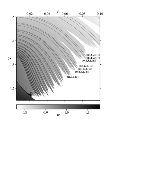
Figure 10: Bird-wing diagram $w(\varepsilon,\nu)$ in the parameter space showing values of the winding number $w$ of the CIC by nuances of the grey color. White zone: regime with broken CTB and cross-jet transport. The curves with irrational winding numbers end up on the tips of the ‘‘feathers of the wing’’ (some of them are marked by the corresponding noble numbers), whereas the curves with rational winding numbers (shown in Fig. 6) end up in the dips of ‘‘the wing’’.

IV Breakdown of central transport barrier

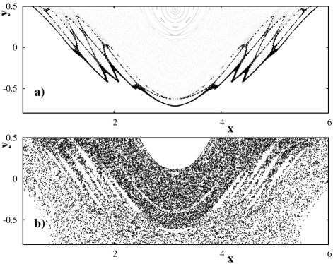
Figure 11: Destruction of central transport barrier upon moving in the parameter space along a resonant bifurcation curve with the rational winding number $w=8/9$. (a) Narrow stochastic layer on the Poincaré section is confined between invariant curves which provide a transport barrier. The perturbation parameters ($\varepsilon=0.04889$, $\nu=1.31625$) are chosen on the curve with $w=8/9$ nearby its right edge (see Fig. 6). (b) Onset of cross-jet transport at the values of parameters ($\varepsilon=0.054$, $\nu=1.285$) chosen in the white zone of that dip.

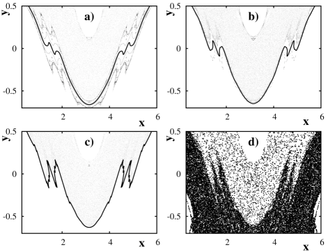
Figure 12: Destruction of central transport barrier upon moving in the parameter space along a curve with the noble value of the CIC’s winding number $w=[0;1,5,1,(1)]$. When approaching a tip of the corresponding ‘‘feather of the wing’’ in Fig. 10, one observes on the Poincaré section a decrease in the width of transport barrier with a CIC (bold curves) inside. (a) $\varepsilon=0.07017$, $\nu=1.367875$. (b) $\varepsilon=0.07416$, $\nu=1.350375$. (c) $\varepsilon=0.0796067$, $\nu=1.325875$. (d) Onset of cross-jet transport at the values of parameters ($\varepsilon=0.08$, $\nu=1.3142$) chosen beyond a tip of that ‘‘feather’’ in the white zone in Fig. 10.

We have studied in the preceding section properties of the CIC which has been shown to be a diagnostic means to characterize CTB and its destruction. CTB separates water masses to the south and the north from the central jet and prevents their mixing. It is not a homogeneous jet-like layer but consists of chains of ballistic islands, narrow stochastic layers, and meandering invariant curves of different orders and periods (including a CIC) to be confined by invariant curves from the south and the north. Those curves break down one after another when increasing the perturbation amplitude $\varepsilon$, producing stochastic layers at their place on both sides of the central jet, until the stochastic layers merge with one another and with stochastic layers around the southern and northern circulation cells producing a global stochastic layer and onset of cross-jet transport.

Upon moving along any resonant bifurcation curve with a rational value of the winding number $w$ in the bird-wing diagram in Fig. 6, we have those values of the perturbation amplitude $\varepsilon$ and frequency $\nu$ at which the corresponding CIC is broken due to reconnection of invariant manifolds. It does not mean that CTB is broken as well. That is the case only if we are at the dips of the ‘‘wing’’. The process of CTB destruction for this type of movement in the parameter space is illustrated in Fig. 11. We fix a point ($\varepsilon=0.04889$, $\nu=1.31625$) on the resonant bifurcation curve with $w=8/9$ nearby its right edge in Fig. 6 and plot the corresponding Poincaré section. A narrow stochastic layer, confined between invariant curves providing a transport barrier, appears on the Poincaré section in panel (a) at the place of a broken CIC. The barrier will be broken if one would choose the values of parameters in the white zone in Fig. 6. Merging of southern and northern stochastic layers and onset of cross-jet transport are shown in panel (b) at $\varepsilon=0.054$, $\nu=1.285$.

Upon moving along any curve with a noble value of the winding number $w$ in the bird-wing diagram in Fig. 10, we have those values of the perturbation amplitude $\varepsilon$ and frequency $\nu$ at which a CIC with the corresponding noble number exists. The process of CTB destruction for the motion in the parameter space along the noble curve with $w=[0;1,5,1,(1)]$ is illustrated in Fig. 12. When moving to the tip of the corresponding ‘‘feather of the wing’’ in Fig. 10, one observes progressive destruction of invariant curves and decrease of the width of the transport barrier (panels (a) and (b)) unless a single CIC remains as the last barrier to cross-jet transport (panel (c)). Onset of cross-jet transport (panel (d)) happens at the values of parameters chosen beyond a tip of that ‘‘feather’’ in the white zone in Fig.10.

Upon moving along any resonant bifurcation curve to the corresponding dip of the bird-wing diagram in Fig. 6, we find cross-jet transport at smaller values of the perturbation amplitude as compared to the case with irrational winding numbers because in order to provide cross-jet transport in the first case it is enough to destruct all the KAM curves. Whereas, CICs with irrational and especially noble values of the winding number may deform in a complicated way but still survive under increasing $\varepsilon$ up to comparatively large values.

V Conclusion

Being motivated by the problem of cross-jet transport in geophysical flows in the ocean and atmosphere, we have studied in detail topology of a central transport barrier (CTB) and its destruction in a simple kinematic model of a meandering current with chaotic advection of passive particles (Fig. 1) that belong to the class of non-degeneracy Hamiltonian systems. Direct computation of the amplitude–frequency diagram (Fig. 2) demonstrated onset of cross-jet transport at surprisingly small values of the perturbation amplitude $\varepsilon$ provided that the perturbation frequency $\nu$ was sufficiently large. As an indicator of the strength of the CTB and its topology, we used a central invariant curve (CIC) which was constructed by iterating indicator points by a numerical procedure borrowed from theory of nontwist maps. The CTB has been shown to exist provided a set of the iterations was bounded. Otherwise, cross-jet transport has been observed (Fig. 3). The results were presented as a diagram of the box-counting dimension of those sets of iterations in Fig. 4.

Geometry of the CIC has been shown to be highly sensitive to small variations in the parameters near a fractal-like boundary of the diagram (Fig. 5). Quantifying complexity of the CIC’s form by its length $L$, we computed the corresponding $L$ diagram looking like a bird wing with a fractal-like boundary (Fig. 6). Resonant bifurcation curves with rational winding numbers $m/n$ end up in the dips of the boundary. Along those curves in the parameter space, invariant manifolds of the corresponding $n:m$ resonances connect providing a destruction of the CIC. Scenarios of the reconnection are different for odd (Fig. 8) and even (Fig. 9) resonances. Animation of the process at http://dynalab.poi.dvo.ru/papers/cic.avi provides a visual demonstration of complexity of topology of the CTB and its destruction. Computing the winding number $w$ of the CIC, we have got an information about those values of the perturbation parameters at which the CTB is strong or weak. Using representation of the values of winding numbers by continued fractions, we were able to order spikes with rational values of $w$ in Fig. 7 into hierarchical series of the corresponding CIC resonances. The curve, which end up on the tips of ‘‘feathers of the wing’’ in the winding-number diagram in Fig. 10, have noble winding numbers which are so irrational that the corresponding CICs break down in the last turn when varying the perturbation parameters. The noble curves have been found to be arranged in series like the resonant bifurcation curves with rational values of $w$. Destruction of CTB is illustrated for two ways in the parameter space: upon moving along resonant bifurcation curves with rational values of $w$ (Fig. 11) and along curves with noble values of $w$ (Fig. 12).

In conclusion we address two points that may be important in possible aplications of the results abtained. Molecular diffusion in laboratory experiment and turbulent diffusion in geophysical flows are expected to wash out ideal fractal-like structures caused by chaotic advection after a characteristic time scale. The question is what is this scale. As to molecular diffusion in the ocean, the diffusion time-scale $L^{2}/D$ is very large since the diffusion coefficient is of the order of $D\simeq 10^{-5}$ cm²/sec and $L$ is of a kilometer scale. The scale of molecular diffusion in laboratory tanks is, of course, much smaller. However, some fractal-like structures have been observed in real laboratory experiments (see, for example, Ref. SKG96 and the book Book08 for a recent review of experiments). Modelling of a combined effect of chaotic advection and turbulent diffusion in the ocean is a hard problem deserving a special consideration. Any kind of diffusion is expected to intensify cross-jet transport.

The advantage of the kinematic approach is its ability to identify different factors that may enhance or suppress cross-jet transport. However, the results obtained with our simplified kinematic model should be taken with caution to describe cross-jet transport in real geophysical flows. In any kinematic model the velocity field is postulated based on known features of the current while in dynamic models it should obey dynamical equations following from the conservation of potential vorticity P87 ; P91 . It is very difficult to formulate an analytic and dynamically consistent model with chaotic advection (for a discussion and examples of such models see DM93 ; P.H.Haynes ; PK06 ; KSD08 ). One approach is to seek solutions of the fluid dynamics equations that are self-consistent to linear order Lipps . Some aspects of cross-jet transport in a linearized model with a zonal Bickley jet current and two Rossby waves have been studied in Refs. DM93 ; PL95 ; Rypina . Potential vorticity is not exactly conserved within the linear approximation but models that are self-consistent to linear order provide a compromise between the self-consistency demands and the fruitfulness of Hamiltonian models.

The question, how predictions of kinematic models in destruction of barriers to cross-jet transport carry over to more realistic dynamical models, remains open. We plan in the future to apply the methods developed in the present paper to a dynamically consistent model of a meandering current with Rossby waves.

References

- (1) V. I. Arnold, C.R. Hebd. Seances Acad. Sci. 261, 17 (1965).
- (2) H. Aref, J. Fluid Mech. 143, 1 (1984).
- (3) H. Aref, Phys. Fluids 14, 1315 (2002).
- (4) J. M. Ottino, Annu. Rev. Fluid Mech. 22, 207 (1990).
- (5) V. I. Arnold, V. V. Kozlov, and A. I. Neishtadt, Mathematical Aspects of Classical and Celestial Mechanics. Encyclopedia of Mathematical Sciences (Springer-Verlag, Berlin, 1988).
- (6) A. J. Lichtenberg and M. A. Lieberman, Regular and Stochastic Motion (Springer-Verlag, New York, 1983).
- (7) E. Ott, Chaos in Dynamical Systems (Cambridge University Press, Cambridge, 1993).
- (8) G. M. Zaslavsky, Hamiltonian Chaos and Fractional Dynamics (University Press, Oxford, 2005).
- (9) R. M. Samelson, J. Phys. Oceanogr. 22, 431 (1992).
- (10) J. Q. Duan and S. Wiggins, J. Phys. Oceanogr. 26, 1176 (1996).
- (11) P. D. Miller, C. K. R. T. Jones, A. M. Rogerson, and L. J. Pratt, Physica D 110, 105 (1997).
- (12) G. C. Yuan, L. J. Pratt, and C. K. R. T. Jones, Dyn. Atmos. Oceans. 35, 41 (2002).
- (13) S. V. Prants, M. V. Budyansky, M. Yu. Uleysky, and G. M. Zaslavsky, Chaos 16, 033117 (2006).
- (14) M. Yu. Uleysky, M. V. Budyansky, and S. V. Prants, Chaos 17, 024703 (2007).
- (15) K. V. Koshel and S. V. Prants, Physics–Uspekhi 49, 1151 (2006).
- (16) K. V. Koshel and S. V. Prants, Chaotic Advection in the Ocean (Institute for Computer Science, Moscow-Izhevsk, 2008) [in Russian].
- (17) A. S. Bower, J. Phys. Oceanogr. 21, 173 (1991).
- (18) S. D. Meyers, J. Phys. Oceanogr. 24, 1641 (1994).
- (19) M. Yu. Uleysky, M. V. Budyansky, and S. V. Prants, Journal of Physics A: Math. Theor. 41, 215102 (2008).
- (20) V. K. Melnikov, Trudi Moskovskogo Obschestva 12, 3 (1963) [Trans. Moscow. Math. Soc.12, 1(1963)].
- (21) B. V. Chirikov, Phys. Rep. 52, 265 (1979).
- (22) G. Boffetta, G. Lacorata, G. Redaelli, and A. Vulpiani, Physica D. 159, 58 (2001).
- (23) F. Raynal and S. Wiggins, Physica D 223, 7 (2006).
- (24) J. Sommeria, S. D. Meyers, and H. L. Swinney, Nature 337, 58 (1989).
- (25) R. P. Behringer, S. D. Meyers, and H. L. Swinney, Phys. Fluids A 3, 1243 (1991).
- (26) T. H. Solomon, W. J. Holloway, and H. L. Swinney, Phys. Fluids A 5, 1971 (1993).
- (27) D. Del-Castillo-Negrete and P. J. Morrison, Phys. Fluids A 5, 948 (1993).
- (28) I. I. Rypina, M. G. Brown, F. J. Beron-Vera, H. Kozak, M. J. Olascoaga, and I. A. Udovydchenkov, J. Atmos. Sci. 64, 3595 (2007).
- (29) P. H. Haynes, D. A. Poet, and E. F. Shuckburgh, J. Atmos. Sci. 64, 3640 (2007).
- (30) G. C. Yuan, L. J. Pratt, and C. K. R. T. Jones, J. Phys. Oceanogr. 34, 1991 (2004).
- (31) J. E. Howard and S. M. Hohs, Phys. Rev. A. 29, 418 (1984).
- (32) A. Wurm, A. Apte, K. Fuchss, and P. J. Morrison, Chaos 15, 023108 (2005).
- (33) S. Shinohara and Y. Aizawa, Progr. of Theor. Phys. 100, 219 (1998).
- (34) A. Wurm, A. Apte, and P. J. Morrison, Brazilian Journal of Physics 34, 1700 (2004).
- (35) S. Shinohara and Y. Aizawa, Progr. of Theor. Phys. 97, 379 (1997).
- (36) J. P. van der Weele, T. P. Valkering, H. W. Capel, and T. Post, Physica A 153, 283 (1998).
- (37) D. del-Castillo-Negrete, J. M. Greene, and P. J. Morrison, Physica D 91, 1 (1996).
- (38) D. del-Castillo-Negrete, J. M. Greene, and P. J. Morrison, Physica D 100, 311 (1997).
- (39) S. M. Soskin, O. M. Yevtushenko, and R. Mannella, Phys. Rev. Let. 90, 174101 (2003).
- (40) S. M. Soskin, R. Mannella, and O. M. Yevtushenko, Phys. Rev. E. 77, 036221 (2008).
- (41) C. Simó, Regular and Chaotic Dynamics 3, 180 (1998).
- (42) A.M. Ozorio de Almeida, Hamiltonian Systems: Chaos and Quantization (Cambridge University Press, Cambridge, 1988).
- (43) J. C. Sommerer, H.-C. Ku, H. E. Gilreath, Phys. Rev. Lett. 77, 5055 (1996).
- (44) J. Pedlosky, Geophysical fluid dynamics (Springer-Verlag, New-York, 1987).
- (45) R. T. Pierrehumbert, Geophys. Astrophys. Fluid Dyn. 58, 285 (1991).
- (46) K.V. Koshel, M.A. Sokolovskiy, and P.A. Davies, Fluid Dynamics Research, 40, 695 (2008).
- (47) F. B. Lipps, Monthly Weather Review 98, 122 (1970).
- (48) L. J. Pratt, M. S. Lozier, and N. Beliakova, J. Phys. Oceanogr. 25, 1451 (1995).