Random complex dynamics and
semigroups of holomorphic maps

Abstract

We investigate the random dynamics of rational maps on the Riemann sphere $\hat{\mathbb{C}}$ and the dynamics of semigroups of rational maps on $\hat{\mathbb{C}}.$ We show that regarding random complex dynamics of polynomials, in most cases, the chaos of the averaged system disappears, due to the cooperation of the generators. We investigate the iteration and spectral properties of transition operators. We show that under certain conditions, in the limit stage, “singular functions on the complex plane” appear. In particular, we consider the functions $T$ which represent the probability of tending to infinity with respect to the random dynamics of polynomials. Under certain conditions these functions $T$ are complex analogues of the devil’s staircase and Lebesgue’s singular functions. More precisely, we show that these functions $T$ are continuous on $\hat{\mathbb{C}}$ and vary only on the Julia sets of associated semigroups. Furthermore, by using ergodic theory and potential theory, we investigate the non-differentiability and regularity of these functions. We find many phenomena which can hold in the random complex dynamics and the dynamics of semigroups of rational maps, but cannot hold in the usual iteration dynamics of a single holomorphic map. We carry out a systematic study of these phenomena and their mechanisms.

1 Introduction

In this paper, we investigate the random dynamics of rational maps on the Riemann sphere $\hat{\mathbb{C}}$ and the dynamics of rational semigroups (i.e., semigroups of non-constant rational maps where the semigroup operation is functional composition) on $\hat{\mathbb{C}}.$ We see that the both fields are related to each other very deeply. In fact, we develop both theories simultaneously.

One motivation for research in complex dynamical systems is to describe some mathematical models on ethology. For example, the behavior of the population of a certain species can be described by the dynamical system associated with iteration of a polynomial $f(z)=az(1-z)$ such that $f$ preserves the unit interval and the postcritical set in the plane is bounded (cf. [7]). However, when there is a change in the natural environment, some species have several strategies to survive in nature. From this point of view, it is very natural and important not only to consider the dynamics of iteration, where the same survival strategy (i.e., function) is repeatedly applied, but also to consider random dynamics, where a new strategy might be applied at each time step. The first study of random complex dynamics was given by J. E. Fornaess and N. Sibony ([9]). For research on random complex dynamics of quadratic polynomials, see [2, 3, 4, 5, 6, 10]. For research on random dynamics of polynomials (of general degrees) with bounded planar postcritical set, see the author’s works [35, 34, 36, 37, 38, 39].

The first study of dynamics of rational semigroups was conducted by A. Hinkkanen and G. J. Martin ([13]), who were interested in the role of the dynamics of polynomial semigroups (i.e., semigroups of non-constant polynomial maps) while studying various one-complex-dimensional moduli spaces for discrete groups, and by F. Ren’s group ([11]), who studied such semigroups from the perspective of random dynamical systems. Since the Julia set $J(G)$ of a finitely generated rational semigroup $G=\langle h_{1},\ldots,h_{m}\rangle$ has “backward self-similarity,” i.e., $J(G)=\bigcup_{j=1}^{m}h_{j}^{-1}(J(G))$ (see Lemma 4.1 and [26, Lemma 1.1.4]), the study of the dynamics of rational semigroups can be regarded as the study of “backward iterated function systems,” and also as a generalization of the study of self-similar sets in fractal geometry.

For recent work on the dynamics of rational semigroups, see the author’s papers [26]–[39], [41], and [25, 42, 43, 44, 45].

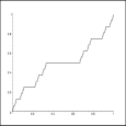
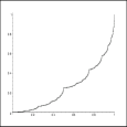
In order to consider the random dynamics of a family of polynomials on $\hat{\mathbb{C}}$, let $T_{\infty}(z)$ be the probability of tending to $\infty\in\hat{\mathbb{C}}$ starting with the initial value $z\in\hat{\mathbb{C}}.$ In this paper, we see that under certain conditions, the function $T_{\infty}:\hat{\mathbb{C}}\rightarrow[0,1]$ is continuous on $\hat{\mathbb{C}}$ and has some singular properties (for instance, varies only on a thin fractal set, the so-called Julia set of a polynomial semigroup), and this function is a complex analogue of the devil’s staircase (Cantor function) or Lebesgue’s singular functions (see Example 6.2, Figures 2, 3, and 4). Before going into detail, let us recall the definition of the devil’s staircase (Cantor function) and Lebesgue’s singular functions. Note that the following definitions look a little bit different from those in [46], but it turns out that they are equivalent to those in [46].

Definition 1.1 ([46]).

Let $\varphi:\mathbb{R}\rightarrow[0,1]$ be the unique bounded function which satisfies the following functional equation:

$$\frac{1}{2}\varphi(3x)+\frac{1}{2}\varphi(3x-2)\equiv\varphi(x),\ \varphi|_{(-\infty,0]}\equiv 0,\ \varphi|_{[1,+\infty)}\equiv 1.$$ (1)

The function $\varphi|_{[0,1]}:[0,1]\rightarrow[0,1]$ is called the devil’s staircase (or Cantor function).

Remark 1.2.

The above $\varphi:\mathbb{R}\rightarrow[0,1]$ is continuous on $\mathbb{R}$ and varies precisely on the Cantor middle third set. Moreover, it is monotone (see Figure 1).

Definition 1.3 ([46]).

Let $0<a<1$ be a constant. We denote by $\psi_{a}:\mathbb{R}\rightarrow[0,1]$ the unique bounded function which satisfies the following functional equation:

$$a\psi_{a}(2x)+(1-a)\psi_{a}(2x-1)\equiv\psi_{a}(x),\ \psi_{a}|_{(-\infty,0]}\equiv 0,\ \psi_{a}|_{[1,+\infty)}\equiv 1.$$ (2)

For each $a\in(0,1)$ with $a\neq 1/2$, the function $L_{a}:=\psi_{a}|_{[0,1]}:[0,1]\rightarrow[0,1]$ is called Lebesgue’s singular function with respect to the parameter $a.$

Remark 1.4.

The function $\psi_{a}:\mathbb{R}\rightarrow[0,1]$ is continuous on $\mathbb{R}$, monotone on $\mathbb{R}$, and strictly monotone on $[0,1]$. Moreover, if $a\neq 1/2$, then for almost every $x\in[0,1]$ with respect to the one-dimensional Lebesgue measure, the derivative of $\psi_{a}$ at $x$ is equal to zero (see Figure 1). For the details on the devil’s staircase and Lebesgue’s singular functions and their related topics, see [46, 12].

Figure 1: (From left to right) The graphs of the devil’s staircase and Lebesgue’s singular function.

These singular functions defined on $[0,1]$ can be redefined by using random dynamical systems on $\mathbb{R}$ as follows. Let $f_{1}(x):=3x,f_{2}(x):=3(x-1)+1\ (x\in\mathbb{R})$ and we consider the random dynamical system (random walk) on $\mathbb{R}$ such that at every step we choose $f_{1}$ with probability $1/2$ and $f_{2}$ with probability $1/2.$ We set $\hat{\mathbb{R}}:=\mathbb{R}\cup\{\pm\infty\}.$ We denote by $T_{+\infty}(x)$ the probability of tending to $+\infty\in\hat{\mathbb{R}}$ starting with the initial value $x\in\mathbb{R}.$ Then, we can see that the function $T_{+\infty}|_{[0,1]}:[0,1]\rightarrow[0,1]$ is equal to the devil’s staircase.

Similarly, let $g_{1}(x):=2x,g_{2}(x):=2(x-1)+1\ (x\in\mathbb{R})$ and let $0<a<1$ be a constant. We consider the random dynamical system on $\mathbb{R}$ such that at every step we choose the map $g_{1}$ with probability $a$ and the map $g_{2}$ with probability $1-a.$ Let $T_{+\infty,a}(x)$ be the probability of tending to $+\infty$ starting with the initial value $x\in\mathbb{R}.$ Then, we can see that the function $T_{+\infty,a}|_{[0,1]}:[0,1]\rightarrow[0,1]$ is equal to Lebesgue’s singular function $L_{a}$ with respect to the parameter $a.$

We remark that in most of the literature, the theory of random dynamical systems has not been used directly to investigate these singular functions on the interval, although some researchers have used it implicitly.

One of the main purposes of this paper is to consider the complex analogue of the above story. In order to do that, we have to investigate the independent and identically-distributed (abbreviated by i.i.d.) random dynamics of rational maps and the dynamics of semigroups of rational maps on $\hat{\mathbb{C}}$ simultaneously. We develop both the theory of random dynamics of rational maps and that of the dynamics of semigroups of rational maps. The author thinks this is the best strategy since when we want to investigate one of them, we need to investigate the other.

To introduce the main idea of this paper, we let $G$ be a rational semigroup and denote by $F(G)$ the Fatou set of $G$, which is defined to be the maximal open subset of $\hat{\mathbb{C}}$ where $G$ is equicontinuous with respect to the spherical distance on $\hat{\mathbb{C}}$. We call $J(G):=\hat{\mathbb{C}}\setminus F(G)$ the Julia set of $G.$ The Julia set is backward invariant under each element $h\in G$, but might not be forward invariant. This is a difficulty of the theory of rational semigroups. Nevertheless, we “utilize” this as follows. The key to investigating random complex dynamics is to consider the following kernel Julia set of $G$, which is defined by $J_{\ker}(G)=\bigcap_{g\in G}g^{-1}(J(G)).$ This is the largest forward invariant subset of $J(G)$ under the action of $G.$ Note that if $G$ is a group or if $G$ is a commutative semigroup, then $J_{\ker}(G)=J(G).$ However, for a general rational semigroup $G$ generated by a family of rational maps $h$ with $\deg(h)\geq 2$, it may happen that $\emptyset=J_{\ker}(G)\neq J(G)$ (see subsection 3.5, section 6).

Let Rat be the space of all non-constant rational maps on the Riemann sphere $\hat{\mathbb{C}}$, endowed with the distance $\kappa$ which is defined by $\kappa(f,g):=\sup_{z\in\hat{\mathbb{C}}}d(f(z),g(z))$, where $d$ denotes the spherical distance on $\hat{\mathbb{C}}.$ Let Rat₊ be the space of all rational maps $g$ with $\deg(g)\geq 2.$ Let ${\cal P}$ be the space of all polynomial maps $g$ with $\deg(g)\geq 2.$ Let $\tau$ be a Borel probability measure on Rat with compact support. We consider the i.i.d. random dynamics on $\hat{\mathbb{C}}$ such that at every step we choose a map $h\in\mbox{Rat}$ according to $\tau.$ Thus this determines a time-discrete Markov process with time-homogeneous transition probabilities on the phase space $\hat{\mathbb{C}}$ such that for each $x\in\hat{\mathbb{C}}$ and each Borel measurable subset $A$ of $\hat{\mathbb{C}}$, the transition probability $p(x,A)$ of the Markov process is defined as $p(x,A)=\tau(\{g\in\text{Rat}\mid g(x)\in A\}).$ Let $G_{\tau}$ be the rational semigroup generated by the support of $\tau.$ Let $C(\hat{\mathbb{C}})$ be the space of all complex-valued continuous functions on $\hat{\mathbb{C}}$ endowed with the supremum norm. Let $M_{\tau}$ be the operator on $C(\hat{\mathbb{C}})$ defined by $M_{\tau}(\varphi)(z)=\int\varphi(g(z))d\tau(g).$ This $M_{\tau}$ is called the transition operator of the Markov process induced by $\tau.$ For a topological space $X$, let ${\mathfrak{M}}_{1}(X)$ be the space of all Borel probability measures on $X$ endowed with the topology induced by the weak convergence (thus $\mu_{n}\rightarrow\mu$ in ${\mathfrak{M}}_{1}(X)$ if and only if $\int\varphi d\mu_{n}\rightarrow\int\varphi d\mu$ for each bounded continuous function $\varphi:X\rightarrow\mathbb{R}$). Note that if $X$ is a compact metric space, then ${\mathfrak{M}}_{1}(X)$ is compact and metrizable. For each $\tau\in{\mathfrak{M}}_{1}(X)$, we denote by supp$\,\tau$ the topological support of $\tau.$ Let ${\mathfrak{M}}_{1,c}(X)$ be the space of all Borel probability measures $\tau$ on $X$ such that supp$\,\tau$ is compact. Let $M_{\tau}^{\ast}:{\mathfrak{M}}_{1}(\hat{\mathbb{C}})\rightarrow{\mathfrak{M}}_{1}(\hat{\mathbb{C}})$ be the dual of $M_{\tau}$. This $M_{\tau}^{\ast}$ can be regarded as the “averaged map” on the extension ${\mathfrak{M}}_{1}(\hat{\mathbb{C}})$ of $\hat{\mathbb{C}}$ (see Remark 2.21). We define the “Julia set” $J_{meas}(\tau)$ of the dynamics of $M_{\tau}^{\ast}$ as the set of all elements $\mu\in{\mathfrak{M}}_{1}(\hat{\mathbb{C}})$ satisfying that for each neighborhood $B$ of $\mu$, $\{(M_{\tau}^{\ast})^{n}|_{B}:B\rightarrow{\mathfrak{M}}_{1}(\hat{\mathbb{C}})\}_{n\in\mathbb{N}}$ is not equicontinuous on $B$ (see Definition 2.17). For each sequence $\gamma=(\gamma_{1},\gamma_{2},\ldots)\in(\text{Rat})^{\mathbb{N}}$, we denote by $J_{\gamma}$ the set of non-equicontinuity of the sequence $\{\gamma_{n}\circ\cdots\circ\gamma_{1}\}_{n\in\mathbb{N}}$ with respect to the spherical distance on $\hat{\mathbb{C}}.$ This $J_{\gamma}$ is called the Julia set of $\gamma.$ Let $\tilde{\tau}:=\otimes_{j=1}^{\infty}\tau\in{\mathfrak{M}}_{1}((\text{Rat})^{\mathbb{N}}).$

We prove the following theorem.

Theorem 1.5 (Cooperation Principle I, see Theorem 3.14 and Proposition 4.7).

Let $\tau\in{\mathfrak{M}}_{1,c}({\text{{\em Rat}}}).$ Suppose that $J_{\ker}(G_{\tau})=\emptyset.$ Then $J_{meas}(\tau)=\emptyset.$ Moreover, for $\tilde{\tau}$-a.e. $\gamma\in(\text{{\em Rat}})^{\mathbb{N}}$, the $2$-dimensional Lebesgue measure of $J_{\gamma}$ is equal to zero.

This theorem means that if all the maps in the support of $\tau$ cooperate, the set of sensitive initial values of the averaged system disappears. Note that for any $h\in\mbox{Rat}_{+}$, $J_{meas}(\delta_{h})\neq\emptyset.$ Thus the above result deals with a phenomenon which can hold in the random complex dynamics but cannot hold in the usual iteration dynamics of a single rational map $h$ with $\deg(h)\geq 2.$

From the above result and some further detailed arguments, we prove the following theorem. To state the theorem, for a $\tau\in{\mathfrak{M}}_{1,c}(\text{Rat})$, we denote by $U_{\tau}$ the space of all finite linear combinations of unitary eigenvectors of $M_{\tau}:C(\hat{\mathbb{C}})\rightarrow C(\hat{\mathbb{C}})$, where an eigenvector is said to be unitary if the absolute value of the corresponding eigenvalue is equal to one. Moreover, we set ${\cal B}_{0,\tau}:=\{\varphi\in C(\hat{\mathbb{C}})\mid M_{\tau}^{n}(\varphi)\rightarrow 0\}.$ Under the above notations, we have the following.

Theorem 1.6 (Cooperation Principle II: Disappearance of Chaos, see Theorem 3.15).

Let $\tau\in{\mathfrak{M}}_{1,c}(\text{{\em Rat}}).$ Suppose that $J_{\ker}(G_{\tau})=\emptyset$ and $J(G_{\tau})\neq\emptyset$. Then we have all of the following statements.

• There exists a direct decomposition $C(\hat{\mathbb{C}})=U_{\tau}\oplus{\cal B}_{0,\tau}$. Moreover, $\dim_{\mathbb{C}}U_{\tau}<\infty$ and ${\cal B}_{0,\tau}$ is a closed subspace of $C(\hat{\mathbb{C}}).$ Moreover, there exists a non-empty $M_{\tau}^{\ast}$-invariant compact subset $A$ of ${\mathfrak{M}}_{1}(\hat{\mathbb{C}})$ with finite topological dimension such that for each $\mu\in{\mathfrak{M}}_{1}(\hat{\mathbb{C}})$, $d((M_{\tau}^{\ast})^{n}(\mu),A)\rightarrow 0$ in ${\mathfrak{M}}_{1}(\hat{\mathbb{C}})$ as $n\rightarrow\infty$. Furthermore, each element of $U_{\tau}$ is locally constant on $F(G_{\tau})$. Therefore each element of $U_{\tau}$ is a continuous function on $\hat{\mathbb{C}}$ which varies only on the Julia set $J(G_{\tau}).$

• For each $z\in\hat{\mathbb{C}}$, there exists a Borel subset ${\cal A}_{z}$ of $(\text{{\em Rat}})^{\mathbb{N}}$ with $\tilde{\tau}({\cal A}_{z})=1$ with the following property.

  • For each $\gamma=(\gamma_{1},\gamma_{2},\ldots)\in{\cal A}_{z}$, there exists a number $\delta=\delta(z,\gamma)>0$ such that $\mbox{diam}(\gamma_{n}\cdots\gamma_{1}(B(z,\delta)))\rightarrow 0$ as $n\rightarrow\infty$, where diam denotes the diameter with respect to the spherical distance on $\hat{\mathbb{C}}$, and $B(z,\delta)$ denotes the ball with center $z$ and radius $\delta.$

• There exists at least one and at most finitely many minimal sets for $(G_{\tau},\hat{\mathbb{C}})$, where we say that a non-empty compact subset $L$ of $\hat{\mathbb{C}}$ is a minimal set for $(G_{\tau},\hat{\mathbb{C}})$ if $L$ is minimal in $\{C\subset\hat{\mathbb{C}}\mid\emptyset\neq C\mbox{ is compact},\forall g\in G_{\tau},g(C)\subset C\}$ with respect to inclusion.

• Let $S_{\tau}$ be the union of minimal sets for $(G_{\tau},\hat{\mathbb{C}})$. Then for each $z\in\hat{\mathbb{C}}$ there exists a Borel subset ${\cal C}_{z}$ of $(\text{{\em Rat}})^{\mathbb{N}}$ with $\tilde{\tau}({\cal C}_{z})=1$ such that for each $\gamma=(\gamma_{1},\gamma_{2},\ldots)\in{\cal C}_{z}$, $d(\gamma_{n}\cdots\gamma_{1}(z),S_{\tau})\rightarrow 0$ as $n\rightarrow\infty.$

This theorem means that if all the maps in the support of $\tau$ cooperate, the chaos of the averaged system disappears. Theorem 1.6 describes new phenomena which can hold in random complex dynamics but cannot hold in the usual iteration dynamics of a single $h\in\mbox{Rat}_{+}.$ For example, for any $h\in\mbox{Rat}_{+}$, if we take a point $z\in J(h)$, where $J(h)$ denotes the Julia set of the semigroup generated by $h$, then for any ball $B$ with $B\cap J(h)\neq\emptyset$, $h^{n}(B)$ expands as $n\rightarrow\infty$, and we have infinitely many minimal sets (periodic cycles) of $h.$

In Theorem 3.15, we completely investigate the structure of $U_{\tau}$ and the set of unitary eigenvalues of $M_{\tau}$ (Theorem 3.15). Using the above result, we show that if $\dim_{\mathbb{C}}U_{\tau}>1$ and int$(J(G_{\tau}))=\emptyset$ where int$(\cdot)$ denotes the set of interior points, then $F(G_{\tau})$ has infinitely many connected components (Theorem 3.15-20). Thus the random complex dynamics can be applied to the theory of dynamics of rational semigroups. The key to proving Theorem 1.6 (Theorem 3.15) is to show that for almost every $\gamma=(\gamma_{1},\gamma_{2},\ldots)\in(\text{Rat})^{\mathbb{N}}$ with respect to $\tilde{\tau}:=\otimes_{j=1}^{\infty}\tau$ and for each compact set $Q$ contained in a connected component $U$ of $F(G_{\tau})$, $\mbox{diam}\gamma_{n}\circ\cdots\circ\gamma_{1}(Q)\rightarrow 0$ as $n\rightarrow\infty.$ This is shown by using careful arguments on the hyperbolic metric of each connected component of $F(G_{\tau}).$ Combining this with the decomposition theorem on “almost periodic operators” on Banach spaces from [18], we prove Theorem 1.6 (Theorem 3.15).

Considering these results, we have the following natural question: “When is the kernel Julia set empty?” Since the kernel Julia set of $G$ is forward invariant under $G$, Montel’s theorem implies that if $\tau$ is a Borel probability measure on ${\cal P}$ with compact support, and if the support of $\tau$ contains an admissible subset of ${\cal P}$ (see Definition 3.54), then $J_{\ker}(G_{\tau})=\emptyset$ (Lemma 3.56). In particular, if the support of $\tau$ contains an interior point with respect to the topology of ${\cal P}$, then $J_{\ker}(G_{\tau})=\emptyset$ (Lemma 3.52). From this result, it follows that for any Borel probability measure $\tau$ on ${\cal P}$ with compact support, there exists a Borel probability measure $\rho$ with finite support, such that $\rho$ is arbitrarily close to $\tau$, such that the support of $\rho$ is arbitrarily close to the support of $\tau$ , and such that $J_{\ker}(G_{\rho})=\emptyset$ (Proposition 3.57). The above results mean that in a certain sense, $J_{\ker}(G_{\tau})=\emptyset$ for most Borel probability measures $\tau$ on ${\cal P}.$ Summarizing these results we can state the following.

Theorem 1.7 (Cooperation Principle III, see Lemmas 3.52, 3.56, Proposition 3.57).

Let ${\mathfrak{M}}_{1,c}({\cal P})$ be endowed with the topology ${\cal O}$ such that $\tau_{n}\rightarrow\tau$ in $({\mathfrak{M}}_{1,c}({\cal P}),{\cal O})$ if and only if (a) $\int\varphi d\tau_{n}\rightarrow\int\varphi d\tau$ for each bounded continuous function $\varphi$ on ${\cal P}$, and (b) supp$\,\tau_{n}\rightarrow$supp$\,\tau$ with respect to the Hausdorff metric. We set $A:=\{\tau\in{\mathfrak{M}}_{1,c}({\cal P})\mid J_{\ker}(G_{\tau})=\emptyset\}$ and $B:=\{\tau\in{\mathfrak{M}}_{1,c}({\cal P})\mid J_{\ker}(G_{\tau})=\emptyset,\sharp\mbox{{\em supp}}\,\tau<\infty\}$. Then we have all of the following.

• $A$ and $B$ are dense in $({\mathfrak{M}}_{1,c}({\cal P}),{\cal O})$.

• If the interior of the support of $\tau$ is not empty with respect to the topology of ${\cal P}$, then $\tau\in A.$

• For each $\tau\in A$, the chaos of the averaged system of the Markov process induced by $\tau$ disappears (more precisely, all the statements in Theorems 1.5, 1.6 hold).

In the subsequent paper [40], we investigate more detail on the above result (some results of [40] are announced in [41]).

We remark that in 1983, by numerical experiments, K. Matsumoto and I. Tsuda ([20]) observed that if we add some uniform noise to the dynamical system associated with iteration of a chaotic map on the unit interval $[0,1]$, then under certain conditions, the quantities which represent chaos (e.g., entropy, Lyapunov exponent, etc.) decrease. More precisely, they observed that the entropy decreases and the Lyapunov exponent turns negative. They called this phenomenon “noise-induced order”, and many physicists have investigated it by numerical experiments, although there has been only a few mathematical supports for it.

Moreover, in this paper, we introduce “mean stable” rational semigroups in subsection 3.6. If $G$ is mean stable, then $J_{\ker}(G)=\emptyset$ and a small perturbation $H$ of $G$ is still mean stable. We show that if $\Gamma$ is a compact subset of Rat₊ and if the semigroup $G$ generated by $\Gamma$ is semi-hyperbolic (see Definition 2.12) and $J_{\ker}(G)=\emptyset$, then there exists a neighborhood ${\cal V}$ of $\Gamma$ in the space of non-empty compact subset of Rat such that for each $\Gamma^{\prime}\in{\cal V}$, the semigroup $G^{\prime}$ generated by $\Gamma^{\prime}$ is mean stable, and $J_{\ker}(G^{\prime})=\emptyset.$

By using the above results, we investigate the random dynamics of polynomials. Let $\tau$ be a Borel probability measure on ${\cal P}$ with compact support. Suppose that $J_{\ker}(G_{\tau})=\emptyset$ and the smallest filled-in Julia set $\hat{K}(G_{\tau})$ (see Definition 3.19) of $G_{\tau}$ is not empty. Then we show that the function $T_{\infty,\tau}$ of probability of tending to $\infty\in\hat{\mathbb{C}}$ belongs to $U_{\tau}$ and is not constant (Theorem 3.22). Thus $T_{\infty,\tau}$ is non-constant and continuous on $\hat{\mathbb{C}}$ and varies only on $J(G_{\tau}).$ Moreover, the function $T_{\infty,\tau}$ is characterized as the unique Borel measurable bounded function $\varphi:\hat{\mathbb{C}}\rightarrow\mathbb{R}$ which satisfies $M_{\tau}(\varphi)=\varphi,$ $\varphi|_{F_{\infty}(G_{\tau})}\equiv 1$, and $\varphi|_{\hat{K}(G_{\tau})}\equiv 0$, where $F_{\infty}(G_{\tau})$ denotes the connected component of the Fatou set $F(G_{\tau})$ of $G_{\tau}$ containing $\infty$ (Proposition 3.26). From these results, we can show that $T_{\infty,\tau}$ has a kind of “monotonicity,” and applying it, we get information regarding the structure of the Julia set $J(G_{\tau})$ of $G_{\tau}$ (Theorem 3.31). We call the function $T_{\infty,\tau}$ a devil’s coliseum, especially when int$(J(G_{\tau}))=\emptyset$ (see Example 6.2, Figures 2, 3, and 4). Note that for any $h\in{\cal P}$, $T_{\infty,\delta_{h}}$ is not continuous at any point of $J(h)\neq\emptyset.$ Thus the above results deal with a phenomenon which can hold in the random complex dynamics, but cannot hold in the usual iteration dynamics of a single polynomial.

It is a natural question to ask about the regularity of non-constant $\varphi\in U_{\tau}$ (e.g., $\varphi=T_{\infty,\tau}$) on the Julia set $J(G_{\tau}).$ For a rational semigroup $G$, we set $P(G):=\overline{\bigcup_{h\in G}\{\mbox{all critical values of }h:\hat{\mathbb{C}}\rightarrow\hat{\mathbb{C}}\}}$, where the closure is taken in $\hat{\mathbb{C}}$, and we say that $G$ is hyperbolic if $P(G)\subset F(G).$ If $G$ is generated by $\{h_{1},\ldots,h_{m}\}$ as a semigroup, we write $G=\langle h_{1},\ldots,h_{m}\rangle.$ We prove the following theorem.

Theorem 1.8 (see Theorem 3.82 and Theorem 3.84).

Let $m\geq 2$ and let $(h_{1},\ldots,h_{m})\in{\cal P}^{m}$. Let $G=\langle h_{1},\ldots,h_{m}\rangle$. Let $0<p_{1},p_{2},\ldots,p_{m}<1$ with $\sum_{i=1}^{m}p_{i}=1.$ Let $\tau=\sum_{i=1}^{m}p_{i}\delta_{h_{i}}.$ Suppose that $h_{i}^{-1}(J(G))\cap h_{j}^{-1}(J(G))=\emptyset$ for each $(i,j)$ with $i\neq j$ and suppose also that $G$ is hyperbolic. Then we have all of the following statements.

• $J_{\ker}(G_{\tau})=\emptyset$, int$(J(G_{\tau}))=\emptyset$, and $\dim_{H}(J(G))<2$, where $\dim_{H}$ denotes the Hausdorff dimension with respect to the spherical distance on $\hat{\mathbb{C}}.$

• Suppose further that at least one of the following conditions (a)(b)(c) holds.

  • $\sum_{j=1}^{m}p_{j}\log(p_{j}\deg(h_{j}))>0.$

  • $P(G)\setminus\{\infty\}$ is bounded in $\mathbb{C}$.

  • $m=2.$

  Then there exists a non-atomic “invariant measure” $\lambda$ on $J(G)$ with supp$\,\lambda=J(G)$ and an uncountable dense subset $A$ of $J(G)$ with $\lambda(A)=1$ and $\dim_{H}(A)>0$, such that for every $z\in A$ and for each non-constant $\varphi\in U_{\tau}$, the pointwise Hölder exponent of $\varphi$ at $z$, which is defined to be

  $$\inf\{\alpha\in\mathbb{R}\mid\limsup_{y\rightarrow z}\frac{|\varphi(y)-\varphi(z)|}{|y-z|^{\alpha}}=\infty\},$$

  is strictly less than $1$ and $\varphi$ is not differentiable at $z$ (Theorem 3.82).

• In (2) above, the pointwise Hölder exponent of $\varphi$ at $z$ can be represented in terms of $p_{j},\log(\deg(h_{j}))$ and the integral of the sum of the values of the Green’s function of the basin of $\infty$ for the sequence $\gamma=(\gamma_{1},\gamma_{2},\ldots)\in\{h_{1},\ldots,h_{m}\}^{\mathbb{N}}$ at the finite critical points of $\gamma_{1}$ (Theorem 3.82).

• Under the assumption of (2), for almost every point $z\in J(G)$ with respect to the $\delta$-dimensional Hausdorff measure $H^{\delta}$ where $\delta=\dim_{H}(J(G))$, the pointwise Hölder exponent of a non-constant $\varphi\in U_{\tau}$ at $z$ can be represented in terms of the $p_{j}$ and the derivatives of $h_{j}$ (Theorem 3.84).

Combining Theorems 1.5, 1.6, 1.8, it follows that under the assumptions of Theorem 1.8, the chaos of the averaged system disappears in the $C^{0}$ “sense”, but it remains in the $C^{1}$ “sense”. From Theorem 1.8, we also obtain that if $p_{1}$ is small enough, then for almost every $z\in J(G)$ with respect to $H^{\delta}$ and for each $\varphi\in U_{\tau}$, $\varphi$ is differentiable at $z$ and the derivative of $\varphi$ at $z$ is equal to zero, even though a non-constant $\varphi\in U_{\tau}$ is not differentiable at any point of an uncountable dense subset of $J(G)$ (Remark 3.86). To prove these results, we use Birkhoff’s ergodic theorem, potential theory, the Koebe distortion theorem and thermodynamic formalisms in ergodic theory. We can construct many examples of $(h_{1},\ldots,h_{m})\in{\cal P}^{m}$ such that $h_{i}^{-1}(J(G))\cap h_{j}^{-1}(J(G))=\emptyset$ for each $(i,j)$ with $i\neq j,$ where $G=\langle h_{1},\ldots,h_{m}\rangle$, $G$ is hyperbolic, $\hat{K}(G)\neq\emptyset$, and $U_{\tau}$ possesses non-constant elements (e.g., $T_{\infty,\tau}$) for any $\tau=\sum_{i=1}^{m}p_{i}\delta_{h_{i}}$ (see Proposition 6.1, Example 6.2, Proposition 6.3, Proposition 6.4, and Remark 6.6).

We also investigate the topology of the Julia sets $J_{\gamma}$ of sequences $\gamma\in(\mbox{supp}\,\tau)^{\mathbb{N}}$, where $\tau$ is a Borel probability measure on ${\cal P}$ with compact support. We show that if $P(G_{\tau})\setminus\{\infty\}$ is not bounded in $\mathbb{C}$, then for almost every sequence $\gamma$ with respect to $\tilde{\tau}:=\otimes_{j=1}^{\infty}\tau$, the Julia set $J_{\gamma}$ of $\gamma$ has uncountably many connected components (Theorem 3.38). This generalizes [2, Theorem 1.5] and [4, Theorem 2.3]. Moreover, we show that $\hat{K}(G_{\tau})=\emptyset$ if and only if $T_{\infty,\tau}\equiv 1$, and that if $\hat{K}(G_{\tau})=\emptyset$, then for almost every $\gamma$ with respect to $\tilde{\tau}$, the $2$-dimensional Lebesgue measure of filled-in Julia set $K_{\gamma}$ (see Definition 3.40) of $\gamma$ is equal to zero and $K_{\gamma}=J_{\gamma}$ has uncountably many connected components (Theorem 3.41 and Example 3.59). These results generalize [4, Theorem 2.2] and one of the statements of [2, Theorem 2.4].

Another matter of considerable interest is what happens when $J_{\ker}(G_{\tau})\neq\emptyset.$ We show that if $\tau$ is a Borel probability measure on Rat₊ with compact support and $G_{\tau}$ is “semi-hyperbolic” (see Definition 2.12), then $J_{\ker}(G_{\tau})\neq\emptyset$ if and only if $J_{meas}(\tau)\neq\emptyset$ (Theorem 3.71). We define several types of “smaller Julia sets” of $M_{\tau}^{\ast}$. We denote by $J_{pt}^{0}(\tau)$ the “pointwise Julia set” of $M_{\tau}^{\ast}$ restricted to $\hat{\mathbb{C}}$ (see Definition 3.44). We show that if $G_{\tau}$ is semi-hyperbolic, then $\dim_{H}(J_{pt}^{0}(\tau))<2$ (Theorem 3.71). Moreover, if $J_{\ker}(G_{\tau})\neq\emptyset$, $G_{\tau}$ is semi-hyperbolic, and $\sharp\mbox{supp}\,\tau<\infty$, then $\overline{J_{pt}^{0}(\tau)}=J(G_{\tau})$ (Theorem 3.71). Thus the dual of the transition operator of the Markov process induced by $\tau$ can detect the Julia set of $G_{\tau}.$ To prove these results, we utilize some observations concerning semi-hyperbolic rational semigroups that may be found in [29, 32]. In particular, the continuity of $\gamma\mapsto J_{\gamma}$ is required. (This is non-trivial, and does not hold for an arbitrary rational semigroup.)

Moreover, even when $J_{\ker}(G_{\tau})\neq\emptyset$, it is shown that if $J_{\ker}(G_{\tau})$ is included in the unbounded component of the complement of the intersection of the set of non-semi-hyperbolic points of $G_{\tau}$ and $J(G_{\tau})$, then for almost every $\gamma\in{\cal P}^{\mathbb{N}}$ with respect to $\tilde{\tau}$, the $2$-dimensional Lebesgue measure of the Julia set $J_{\gamma}$ of $\gamma$ is equal to zero (Theorem 3.48). To prove this result, we again utilize observations concerning the kernel Julia set of $G_{\tau}$, and non-constant limit functions must be handled carefully (Lemmas 4.6, 5.32 and 5.33).

As pointed out in the previous paragraphs, we find many new phenomena which can hold in random complex dynamics and the dynamics of rational semigroups, but cannot hold in the usual iteration dynamics of a single rational map. These new phenomena and their mechanisms are systematically investigated.

In the proofs of all results, we employ the skew product map associated with the support of $\tau$ (Definition 3.46), and some detailed observations concerning the skew product are required. It is a new idea to use the kernel Julia set of the associated semigroup to investigate random complex dynamics. Moreover, it is both natural and new to combine the theory of random complex dynamics and the theory of rational semigroups. Without considering the Julia sets of rational semigroups, we are unable to discern the singular properties of the non-constant finite linear combinations $\varphi$ (e.g., $\varphi=T_{\infty,\tau}$, a devil’s coliseum) of the unitary eigenvectors of $M_{\tau}$.

In section 2, we give some fundamental notations and definitions. In section 3, we present the main results of this paper. In section 4, we introduce the basic tools used to prove the main results. In section 5, we provide the proofs of the main results. In section 6, we give many examples to which the main results are applicable.

In the subsequent paper [40], we investigate the stability and bifurcation of $M_{\tau}$ (some results of [40] are announced in [41]).

Acknowledgment: The author thanks Rich Stankewitz for valuable comments. This work was supported by JSPS Grant-in-Aid for Scientific Research(C) 21540216.

2 Preliminaries

In this section, we give some basic definitions and notations on the dynamics of semigroups of holomorphic maps and the i.i.d. random dynamics of holomorphic maps.

Notation: Let $(X,d)$ be a metric space, $A$ a subset of $X$, and $r>0$. We set $B(A,r):=\{z\in X\mid d(z,A)<r\}.$ Moreover, for a subset $C$ of $\mathbb{C}$, we set $D(C,r):=\{z\in\mathbb{C}\mid\inf_{a\in C}|z-a|<r\}.$ Moreover, for any topological space $Y$ and for any subset $A$ of $Y$, we denote by int$(A)$ the set of all interior points of $A.$

Definition 2.1.

Let $Y$ be a metric space. We set $\text{CM}(Y):=\{f:Y\rightarrow Y\mid f\mbox{ is continuous}\}$ endowed with the compact-open topology. Moreover, we set $\text{OCM}(Y):=\{f\in\text{CM}(Y)\mid f\mbox{ is an open map}\}$ endowed with the relative topology from $\text{CM}(Y).$ Furthermore, we set $C(Y):=\{\varphi:Y\rightarrow\mathbb{C}\mid\varphi\mbox{ is continuous }\}.$ When $Y$ is compact, we endow $C(Y)$ with the supremum norm $\|\cdot\|_{\infty}.$ Moreover, for a subset ${\cal F}$ of $C(Y)$, we set ${\cal F}_{nc}:=\{\varphi\in{\cal F}\mid\varphi\mbox{ is not constant}\}.$

Definition 2.2.

Let $Y$ be a complex manifold. We set $\text{HM}(Y):=\{f:Y\rightarrow Y\mid f\mbox{ is holomorphic}\}$ endowed with the compact open topology. Moreover, we set $\text{NHM}(Y):=\{f\in\text{HM}(Y)\mid f\mbox{ is not constant}\}$ endowed with the compact open topology.

Remark 2.3.

$\text{CM}(Y)$, $\text{OCM}(Y)$, $\text{HM}(Y)$, and $\text{NHM}(Y)$ are semigroups with the semigroup operation being functional composition.

Definition 2.4.

A rational semigroup is a semigroup generated by a family of non-constant rational maps on the Riemann sphere $\hat{\mathbb{C}}$ with the semigroup operation being functional composition([13, 11]). A polynomial semigroup is a semigroup generated by a family of non-constant polynomial maps. We set Rat : $=\{h:\hat{\mathbb{C}}\rightarrow\hat{\mathbb{C}}\mid h\mbox{ is a non-constant rational map}\}$ endowed with the distance $\kappa$ which is defined by $\kappa(f,g):=\sup_{z\in\hat{\mathbb{C}}}d(f(z),g(z))$, where $d$ denotes the spherical distance on $\hat{\mathbb{C}}.$ Moreover, we set $\text{Rat}_{+}:=\{h\in\mbox{Rat}\mid\deg(h)\geq 2\}$ endowed with the relative topology from Rat. Furthermore, we set ${\cal P}:=\{g:\hat{\mathbb{C}}\rightarrow\hat{\mathbb{C}}\mid g\mbox{ is a polynomial},\deg(g)\geq 2\}$ endowed with the relative topology from Rat.

Definition 2.5.

Let $Y$ be a compact metric space and let $G$ be a subsemigroup of $\text{CM}(Y).$ The Fatou set of $G$ is defined to be $F(G):=\\ \{z\in Y\mid\exists\mbox{ neighborhood }U\mbox{ of }z$ s.t. $\{g|_{U}:U\rightarrow Y\}_{g\in G}$ is equicontinuous on $U\}.$ (For the definition of equicontinuity, see [1].) The Julia set of $G$ is defined to be $J(G):=Y\setminus F(G).$ If $G$ is generated by $\{g_{i}\}_{i}$, then we write $G=\langle g_{1},g_{2},\ldots\rangle.$ If $G$ is generated by a subset $\Gamma$ of $\text{CM}(Y)$, then we write $G=\langle\Gamma\rangle.$ For finitely many elements $g_{1},\ldots,g_{m}\in\text{CM}(Y)$, we set $F(g_{1},\ldots,g_{m}):=F(\langle g_{1},\ldots,g_{m}\rangle)$ and $J(g_{1},\ldots,g_{m}):=J(\langle g_{1},\ldots,g_{m}\rangle)$. For a subset $A$ of $Y$, we set $G(A):=\bigcup_{g\in G}g(A)$ and $G^{-1}(A):=\bigcup_{g\in G}g^{-1}(A).$ We set $G^{\ast}:=G\cup\{\mbox{Id}\}$, where Id denotes the identity map.

By using the method in [13, 11], it is easy to see that the following lemma holds.

Lemma 2.6.

Let $Y$ be a compact metric space and let $G$ be a subsemigroup of $\text{{\em OCM}}(Y).$ Then for each $h\in G$, $h(F(G))\subset F(G)$ and $h^{-1}(J(G))\subset J(G).$ Note that the equality does not hold in general.

The following is the key to investigating random complex dynamics.

Definition 2.7.

Let $Y$ be a compact metric space and let $G$ be a subsemigroup of $\text{CM}(Y).$ We set $J_{\ker}(G):=\bigcap_{g\in G}g^{-1}(J(G)).$ This is called the kernel Julia set of $G.$

Remark 2.8.

Let $Y$ be a compact metric space and let $G$ be a subsemigroup of $\text{CM}(Y).$ (1) $J_{\ker}(G)$ is a compact subset of $J(G).$ (2) For each $h\in G$, $h(J_{\ker}(G))\subset J_{\ker}(G).$ (3) If $G$ is a rational semigroup and if $F(G)\neq\emptyset$, then int$(J_{\ker}(G))=\emptyset.$ (4) If $G$ is generated by a single map or if $G$ is a group, then $J_{\ker}(G)=J(G).$ However, for a general rational semigroup $G$, it may happen that $\emptyset=J_{\ker}(G)\neq J(G)$ (see subsection 3.5 and section 6).

The following postcritical set is important when we investigate the dynamics of rational semigroups.

Definition 2.9.

For a rational semigroup $G$, let $P(G):=\overline{\bigcup_{g\in G}\{\mbox{all critical values of }g:\hat{\mathbb{C}}\rightarrow\hat{\mathbb{C}}\}}$ where the closure is taken in $\hat{\mathbb{C}}.$ This is called the postcritical set of $G.$

Remark 2.10.

If $\Gamma\subset\mbox{Rat}$ and $G=\langle\Gamma\rangle$, then $P(G)=\overline{G^{\ast}(\bigcup_{h\in\Gamma}\{\mbox{all critical values of }h\})}.$ From this one may know the figure of $P(G)$, in the finitely generated case, using a computer.

Definition 2.11.

Let $G$ be a rational semigroup. Let $N$ be a positive integer. We denote by $SH_{N}(G)$ the set of points $z\in\hat{\mathbb{C}}$ satisfying that there exists a positive number $\delta$ such that for each $g\in G$, $\deg(g:V\rightarrow B(z,\delta))\leq N$, for each connected component $V$ of $g^{-1}(B(z,\delta)).$ Moreover, we set $UH(G):=\hat{\mathbb{C}}\setminus\bigcup_{N\in\mathbb{N}}SH_{N}(G).$

Definition 2.12.

Let $G$ be a rational semigroup. We say that $G$ is hyperbolic if $P(G)\subset F(G).$ We say that $G$ is semi-hyperbolic if $UH(G)\subset F(G).$

Remark 2.13.

We have $UH(G)\subset P(G).$ If $G$ is hyperbolic, then $G$ is semi-hyperbolic.

It is sometimes important to investigate the dynamics of sequences of maps.

Definition 2.14.

Let $Y$ be a compact metric space. For each $\gamma=(\gamma_{1},\gamma_{2},\ldots)\in(\text{CM}(Y))^{\mathbb{N}}$ and each $m,n\in\mathbb{N}$ with $m\geq n$, we set $\gamma_{m,n}=\gamma_{m}\circ\cdots\circ\gamma_{n}$ and we set

$$F_{\gamma}:=\{z\in Y\mid\exists\mbox{ neighborhood }U\mbox{ of }z\mbox{ s.t. }\{\gamma_{n,1}\}_{n\in\mathbb{N}}\mbox{ is equicontinuous on }U\}$$

and $J_{\gamma}:=Y\setminus F_{\gamma}.$ The set $F_{\gamma}$ is called the Fatou set of the sequence $\gamma$ and the set $J_{\gamma}$ is called the Julia set of the sequence $\gamma.$

Remark 2.15.

Let $Y=\hat{\mathbb{C}}$ and let $\gamma\in(\text{Rat}_{+})^{\mathbb{N}}$. Then by [1, Theorem 2.8.2], $J_{\gamma}\neq\emptyset.$ Moreover, if $\Gamma$ is a non-empty compact subset of $\text{Rat}_{+}$ and $\gamma\in\Gamma^{\mathbb{N}}$, then by [29], $J_{\gamma}$ is a perfect set and $J_{\gamma}$ has uncountably many points.

We now give some notations on random dynamics.

Definition 2.16.

For a topological space $Y$, we denote by ${\mathfrak{M}}_{1}(Y)$ the space of all Borel probability measures on $Y$ endowed with the topology such that $\mu_{n}\rightarrow\mu$ in ${\mathfrak{M}}_{1}(Y)$ if and only if for each bounded continuous function $\varphi:Y\rightarrow\mathbb{C}$, $\int\varphi\ d\mu_{n}\rightarrow\int\varphi\ d\mu.$ Note that if $Y$ is a compact metric space, then ${\mathfrak{M}}_{1}(Y)$ is a compact metric space with the metric $d_{0}(\mu_{1},\mu_{2}):=\sum_{j=1}^{\infty}\frac{1}{2^{j}}\frac{|\int\phi_{j}d\mu_{1}-\int\phi_{j}d\mu_{2}|}{1+|\int\phi_{j}d\mu_{1}-\int\phi_{j}d\mu_{2}|}$, where $\{\phi_{j}\}_{j\in\mathbb{N}}$ is a dense subset of $C(Y).$ Moreover, for each $\tau\in{\mathfrak{M}}_{1}(Y)$, we set $\text{supp}\,\tau:=\{z\in Y\mid\forall\mbox{ neighborhood }U\mbox{ of }z,\ \tau(U)>0\}.$ Note that $\text{supp}\,\tau$ is a closed subset of $Y.$ Furthermore, we set ${\mathfrak{M}}_{1,c}(Y):=\{\tau\in{\mathfrak{M}}_{1}(Y)\mid\text{supp}\,\tau\mbox{ is compact}\}.$

For a complex Banach space ${\cal B}$, we denote by ${\cal B}^{\ast}$ the space of all continuous complex linear functionals $\rho:{\cal B}\rightarrow\mathbb{C}$, endowed with the weak^∗ topology.

For any $\tau\in{\mathfrak{M}}_{1}(\text{CM}(Y))$, we will consider the i.i.d. random dynamics on $Y$ such that at every step we choose a map $g\in\text{CM}(Y)$ according to $\tau$ (thus this determines a time-discrete Markov process with time-homogeneous transition probabilities on the phase space $Y$ such that for each $x\in Y$ and each Borel measurable subset $A$ of $Y$, the transition probability $p(x,A)$ of the Markov process is defined as $p(x,A)=\tau(\{g\in\text{CM}(Y)\mid g(x)\in A\})$).

Definition 2.17.

Let $Y$ be a compact metric space. Let $\tau\in{\mathfrak{M}}_{1}(\text{CM}(Y)).$

1. We set $\Gamma_{\tau}:=\mbox{supp}\,\tau$ (thus $\Gamma_{\tau}$ is a closed subset of $\text{CM}(Y)$). Moreover, we set $X_{\tau}:=(\Gamma_{\tau})^{\mathbb{N}}$ $(=\{\gamma=(\gamma_{1},\gamma_{2},\ldots)\mid\gamma_{j}\in\Gamma_{\tau}\ (\forall j)\})$ endowed with the product topology. Furthermore, we set $\tilde{\tau}:=\otimes{}_{j=1}^{\infty}\tau.$ This is the unique Borel probability measure on $X_{\tau}$ such that for each cylinder set $A=A_{1}\times\cdots\times A_{n}\times\Gamma_{\tau}\times\Gamma_{\tau}\times\cdots$ in $X_{\tau}$, $\tilde{\tau}(A)=\prod_{j=1}^{n}\tau(A_{j}).$ We denote by $G_{\tau}$ the subsemigroup of $\text{CM}(Y)$ generated by the subset $\Gamma_{\tau}$ of $\text{CM}(Y).$

2. Let $M_{\tau}$ be the operator on $C(Y)$ defined by $M_{\tau}(\varphi)(z):=\int_{\Gamma_{\tau}}\varphi(g(z))\ d\tau(g).$ $M_{\tau}$ is called the transition operator of the Markov process induced by $\tau.$ Moreover, let $M_{\tau}^{\ast}:C(Y)^{\ast}\rightarrow C(Y)^{\ast}$ be the dual of $M_{\tau}$, which is defined as $M_{\tau}^{\ast}(\mu)(\varphi)=\mu(M_{\tau}(\varphi))$ for each $\mu\in C(Y)^{\ast}$ and each $\varphi\in C(Y).$ Remark: we have $M_{\tau}^{\ast}({\mathfrak{M}}_{1}(Y))\subset{\mathfrak{M}}_{1}(Y)$ and for each $\mu\in{\mathfrak{M}}_{1}(Y)$ and each open subset $V$ of $Y$, we have $M_{\tau}^{\ast}(\mu)(V)=\int_{\Gamma_{\tau}}\mu(g^{-1}(V))\ d\tau(g).$

3. We denote by $F_{meas}(\tau)$ the set of $\mu\in{\mathfrak{M}}_{1}(Y)$ satisfying that there exists a neighborhood $B$ of $\mu$ in ${\mathfrak{M}}_{1}(Y)$ such that the sequence $\{(M_{\tau}^{\ast})^{n}|_{B}:B\rightarrow{\mathfrak{M}}_{1}(Y)\}_{n\in\mathbb{N}}$ is equicontinuous on $B.$ We set $J_{meas}(\tau):={\mathfrak{M}}_{1}(Y)\setminus F_{meas}(\tau).$

4. We denote by $F_{meas}^{0}(\tau)$ the set of $\mu\in{\mathfrak{M}}_{1}(Y)$ satisfying that the sequence$\{(M_{\tau}^{\ast})^{n}:{\mathfrak{M}}_{1}(Y)\rightarrow{\mathfrak{M}}_{1}(Y)\}_{n\in\mathbb{N}}$ is equicontinuous at the one point $\mu.$ We set $J_{meas}^{0}(\tau):={\mathfrak{M}}_{1}(Y)\setminus F_{meas}^{0}(\tau).$

Remark 2.18.

We have $F_{meas}(\tau)\subset F_{meas}^{0}(\tau)$ and $J_{meas}^{0}(\tau)\subset J_{meas}(\tau).$

Remark 2.19.

Let $\Gamma$ be a closed subset of Rat. Then there exists a $\tau\in{\mathfrak{M}}_{1}(\mbox{Rat})$ such that $\Gamma_{\tau}=\Gamma.$ By using this fact, we sometimes apply the results on random complex dynamics to the study of the dynamics of rational semigroups.

Definition 2.20.

Let $Y$ be a compact metric space. Let $\Phi:Y\rightarrow{\mathfrak{M}}_{1}(Y)$ be the topological embedding defined by: $\Phi(z):=\delta_{z}$, where $\delta_{z}$ denotes the Dirac measure at $z.$ Using this topological embedding $\Phi:Y\rightarrow{\mathfrak{M}}_{1}(Y)$, we regard $Y$ as a compact subset of ${\mathfrak{M}}_{1}(Y).$

Remark 2.21.

If $h\in\text{CM}(Y)$ and $\tau=\delta_{h}$, then we have $M_{\tau}^{\ast}\circ\Phi=\Phi\circ h$ on $Y.$ Moreover, for a general $\tau\in{\mathfrak{M}}_{1}(\text{CM}(Y))$, $M_{\tau}^{\ast}(\mu)=\int h_{\ast}(\mu)d\tau(h)$ for each $\mu\in{\mathfrak{M}}_{1}(Y).$ Therefore, for a general $\tau\in{\mathfrak{M}}_{1}(\text{CM}(Y))$, the map $M_{\tau}^{\ast}:{\mathfrak{M}}_{1}(Y)\rightarrow{\mathfrak{M}}_{1}(Y)$ can be regarded as the “averaged map” on the extension ${\mathfrak{M}}_{1}(Y)$ of $Y.$

Remark 2.22.

If $\tau=\delta_{h}\in{\mathfrak{M}}_{1}(\text{Rat}_{+})$ with $h\in\text{Rat}_{+}$, then $J_{meas}(\tau)\neq\emptyset$. In fact, using the embedding $\Phi:\hat{\mathbb{C}}\rightarrow{\mathfrak{M}}_{1}(\hat{\mathbb{C}})$, we have $\emptyset\neq\Phi(J(h))\subset J_{meas}(\tau).$

The following is an important and interesting object in random dynamics.

Definition 2.23.

Let $Y$ be a compact metric space and let $A$ be a subset of $Y.$ Let $\tau\in{\mathfrak{M}}_{1}(\text{CM}(Y)).$ For each $z\in Y$, we set $T_{A,\tau}(z):=\tilde{\tau}(\{\gamma=(\gamma_{1},\gamma_{2},\ldots)\in X_{\tau}\mid d(\gamma_{n,1}(z),A)\rightarrow 0\mbox{ as }n\rightarrow\infty\}).$ This is the probability of tending to $A$ starting with the initial value $z\in Y.$ For any $a\in Y$, we set $T_{a,\tau}:=T_{\{a\},\tau}.$

3 Results

In this section, we present the main results of this paper.

3.1 General results and properties of $M_{\tau}$

In this subsection, we present some general results and some results on properties of the iteration of $M_{\tau}:C(\hat{\mathbb{C}})\rightarrow C(\hat{\mathbb{C}})$ and $M_{\tau}^{\ast}:C(\hat{\mathbb{C}})^{\ast}\rightarrow C(\hat{\mathbb{C}})^{\ast}.$ The proofs are given in subsection 5.1. We need some notations.

Definition 3.1.

Let $Y$ be a $n$-dimensional smooth manifold. We denote by Leb_n the two-dimensional Lebesgue measure on $Y.$

Definition 3.2.

Let ${\cal B}$ be a complex vector space and let $M:{\cal B}\rightarrow{\cal B}$ be a linear operator. Let $\varphi\in{\cal B}$ and $a\in\mathbb{C}$ be such that $\varphi\neq 0,|a|=1$, and $M(\varphi)=a\varphi.$ Then we say that $\varphi$ is a unitary eigenvector of $M$ with respect to $a$, and we say that $a$ is a unitary eigenvalue.

Definition 3.3.

Let $Y$ be a compact metric space and let $\tau\in{\mathfrak{M}}_{1}(\text{CM}(Y)).$ Let $K$ be a non-empty subset of $Y$ such that $G(K)\subset K$. We denote by ${\cal U}_{f,\tau}(K)$ the set of all unitary eigenvectors of $M_{\tau}:C(K)\rightarrow C(K)$. Moreover, we denote by ${\cal U}_{v,\tau}(K)$ the set of all unitary eigenvalues of $M_{\tau}:C(K)\rightarrow C(K).$ Similarly, we denote by ${\cal U}_{f,\tau,\ast}(K)$ the set of all unitary eigenvectors of $M_{\tau}^{\ast}:C(K)^{\ast}\rightarrow C(K)^{\ast}$, and we denote by ${\cal U}_{v,\tau,\ast}(K)$ the set of all unitary eigenvalues of $M_{\tau}^{\ast}:C(K)^{\ast}\rightarrow C(K)^{\ast}.$

Definition 3.4.

Let $V$ be a complex vector space and let $A$ be a subset of $V.$ We set $\mbox{LS}(A):=\{\sum_{j=1}^{m}a_{j}v_{j}\mid a_{1},\ldots,a_{m}\in\mathbb{C},v_{1},\ldots,v_{m}\in A,m\in\mathbb{N}\}.$

Definition 3.5.

Let $Y$ be a topological space and let $V$ be a subset of $Y.$ We denote by $C_{V}(Y)$ the space of all $\varphi\in C(Y)$ such that for each connected component $U$ of $V$, there exists a constant $c_{U}\in\mathbb{C}$ with $\varphi|_{U}\equiv c_{U}.$

Remark 3.6.

$C_{V}(Y)$ is a linear subspace of $C(Y).$ Moreover, if $Y$ is compact, metrizable, and locally connected and $V$ is an open subset of $Y$, then $C_{V}(Y)$ is a closed subspace of $C(Y).$ Furthermore, if $Y$ is compact, metrizable, and locally connected, $\tau\in{\mathfrak{M}}_{1}(\text{CM}(Y))$, and $G_{\tau}$ is a subsemigroup of $\text{OCM}(Y)$, then $M_{\tau}(C_{F(G_{\tau})}(Y))\subset C_{F(G_{\tau})}(Y).$

Definition 3.7.

For a topological space $Y$, we denote by Cpt$(Y)$ the space of all non-empty compact subsets of $Y$. If $Y$ is a metric space, we endow Cpt$(Y)$ with the Hausdorff metric.

Definition 3.8.

Let $Y$ be a metric space and let $G$ be a subsemigroup of $\text{CM}(Y).$ Let $K\in\text{Cpt}(Y).$ We say that $K$ is a minimal set for $(G,Y)$ if $K$ is minimal among the space $\{L\in\text{Cpt}(Y)\mid G(L)\subset L\}$ with respect to inclusion. Moreover, we set $\text{Min}(G,Y):=\{K\in\text{Cpt}(Y)\mid K\mbox{ is a minimal set for }(G,Y)\}.$

Remark 3.9.

Let $Y$ be a metric space and let $G$ be a subsemigroup of $\text{CM}(Y).$ By Zorn’s lemma, it is easy to see that if $K_{1}\in\text{Cpt}(Y)$ and $G(K_{1})\subset K_{1}$, then there exists a $K\in\text{Min}(G,Y)$ with $K\subset K_{1}.$ Moreover, it is easy to see that for each $K\in\text{Min}(G,Y)$ and each $z\in K$, $\overline{G(z)}=K.$ In particular, if $K_{1},K_{2}\in\text{Min}(G,Y)$ with $K_{1}\neq K_{2}$, then $K_{1}\cap K_{2}=\emptyset.$ Moreover, by the formula $\overline{G(z)}=K$, we obtain that for each $K\in\text{Min}(G,Y)$, either (1) $\sharp K<\infty$ or (2) $K$ is perfect and $\sharp K>\aleph_{0}.$ Furthermore, it is easy to see that if $\Gamma\in\text{Cpt}(\text{CM}(Y)),G=\langle\Gamma\rangle$, and $K\in\text{Min}(G,Y)$, then $K=\bigcup_{h\in\Gamma}h(K).$

Definition 3.10.

Let $Y$ be a compact metric space. Let $\rho\in C(Y)^{\ast}.$ We denote by $a(\rho)$ the set of points $z\in Y$ which satisfies that there exists a neighborhood $U$ of $z$ in $Y$ such that for each $\varphi\in C(Y)$ with $\mbox{supp}\,\varphi\subset U$, $\rho(\varphi)=0.$ We set $\mbox{supp}\,\rho:=Y\setminus a(\rho).$

Definition 3.11.

Let $\{\varphi_{n}:U\rightarrow\hat{\mathbb{C}}\}_{n=1}^{\infty}$ be a sequence of holomorphic maps on an open set $U$ of $\hat{\mathbb{C}}.$ Let $\varphi:U\rightarrow\hat{\mathbb{C}}$ be a holomorphic map. We say that $\varphi$ is a limit function of $\{\varphi_{n}\}_{n=1}^{\infty}$ if there exists a strictly increasing sequence $\{n_{j}\}_{j=1}^{\infty}$ in $\mathbb{N}$ such that $\varphi_{n_{j}}\rightarrow\varphi$ as $j\rightarrow\infty$ locally uniformly on $U.$

Definition 3.12.

For a topological space $Z$, we denote by Con$(Z)$ the set of all connected components of $Z.$

Definition 3.13.

Let $G$ be a rational semigroup. We set $J_{res}(G):=\{z\in J(G)\mid\forall U\in\mbox{Con}(F(G)),z\not\in\partial U\}.$ This is called the residual Julia set of $G.$

We now present the main results.

Theorem 3.14 (Cooperation Principle I).

Let $\tau\in{\mathfrak{M}}_{1,c}(\text{{\em NHM}}(\mathbb{C}\mathbb{P}^{n}))$, where $\mathbb{C}\mathbb{P}^{n}$ denotes the $n$-dimensional complex projective space. Suppose that $J_{\ker}(G_{\tau})=\emptyset.$ Then, $F_{meas}(\tau)={\mathfrak{M}}_{1}(\mathbb{C}\mathbb{P}^{n})$, and for $\tilde{\tau}$-a.e. $\gamma\in(\mbox{{\em NHM}}(\mathbb{C}\mathbb{P}^{n}))^{\mathbb{N}}$, $\mbox{{\em Leb}}_{2n}(J_{\gamma})=0.$

Theorem 3.15 (Cooperation Principle II: Disappearance of Chaos).

Let $\tau\in{\mathfrak{M}}_{1,c}(\text{{\em Rat}})$ and let $S_{\tau}:=\bigcup_{L\in\text{\em Min}(G_{\tau},\hat{\mathbb{C}})}L.$ Suppose that $J_{\ker}(G_{\tau})=\emptyset$ and $J(G_{\tau})\neq\emptyset$. Then, all of the following statements 1,$\ldots,$21 hold.

1. Let ${\cal B}_{0,\tau}:=\{\varphi\in C(\hat{\mathbb{C}})\mid M_{\tau}^{n}(\varphi)\rightarrow 0\mbox{ as }n\rightarrow\infty\}.$ Then, ${\cal B}_{0,\tau}$ is a closed subspace of $C(\hat{\mathbb{C}})$ and there exists a direct sum decomposition $C(\hat{\mathbb{C}})=\mbox{{\em LS}}({\cal U}_{f,\tau}(\hat{\mathbb{C}}))\oplus{\cal B}_{0,\tau}.$ Moreover, $\mbox{{\em LS}}({\cal U}_{f,\tau}(\hat{\mathbb{C}}))\subset C_{F(G_{\tau})}(\hat{\mathbb{C}})$ and $\dim_{\mathbb{C}}(\mbox{{\em LS}}({\cal U}_{f,\tau}(\hat{\mathbb{C}})))<\infty.$

2. Let $q:=\dim_{\mathbb{C}}(\text{{\em LS}}({\cal U}_{f,\tau}(\hat{\mathbb{C}}))).$ Let $\{\varphi_{j}\}_{j=1}^{q}$ be a basis of $\text{{\em LS}}({\cal U}_{f,\tau}(\hat{\mathbb{C}}))$ such that for each $j=1,\ldots,q$, there exists an $\alpha_{j}\in{\cal U}_{v,\tau}(\hat{\mathbb{C}})$ with $M_{\tau}(\varphi_{j})=\alpha_{j}\varphi_{j}.$ Then, there exists a unique family $\{\rho_{j}:C(\hat{\mathbb{C}})\rightarrow\mathbb{C}\}_{j=1}^{q}$ of complex linear functionals such that for each $\varphi\in C(\hat{\mathbb{C}})$, $\|M_{\tau}^{n}(\varphi-\sum_{j=1}^{q}\rho_{j}(\varphi)\varphi_{j})\|_{\infty}\rightarrow 0$ as $n\rightarrow\infty.$ Moreover, $\{\rho_{j}\}_{j=1}^{q}$ satisfies all of the following.

   • For each $j=1,\ldots,q$, $\rho_{j}:C(\hat{\mathbb{C}})\rightarrow\mathbb{C}$ is continuous.

   • For each $j=1,\ldots,q$, $M_{\tau}^{\ast}(\rho_{j})=\alpha_{j}\rho_{j}.$

   • For each $(i,j)$, $\rho_{i}(\varphi_{j})=\delta_{ij}.$ Moreover, $\{\rho_{j}\}_{j=1}^{q}$ is a basis of $\text{{\em LS}}({\cal U}_{f,\tau,\ast}(\hat{\mathbb{C}})).$

   • For each $j=1,\ldots,q$, supp$\,\rho_{j}\subset S_{\tau}.$

3. We have $\sharp J(G_{\tau})\geq 3.$ In particular, for each $U\in\mbox{{\em Con}}(F(G_{\tau}))$, we can take the hyperbolic metric on $U.$

4. There exists a Borel measurable subset ${\cal A}$ of $(\text{{\em Rat}})^{\mathbb{N}}$ with $\tilde{\tau}({\cal A})=1$ such that

   • for each $\gamma\in{\cal A}$ and for each $U\in\mbox{{\em Con}}(F(G_{\tau}))$, each limit function of $\{\gamma_{n,1}|_{U}\}_{n=1}^{\infty}$ is constant, and

   • for each $\gamma\in{\cal A}$ and for each $Q\in\mbox{{\em Cpt}}(F(G_{\tau}))$, $\sup_{a\in Q}\|\gamma_{n,1}^{\prime}(a)\|_{h}\rightarrow 0$ as $n\rightarrow\infty$, where $\|\gamma_{n,1}^{\prime}(a)\|_{h}$ denotes the norm of the derivative of $\gamma_{n,1}$ at a point $a$ measured from the hyperbolic metric on the element $U_{0}\in\mbox{{\em Con}}(F(G_{\tau}))$ with $a\in U_{0}$ to that on the element $U_{n}\in\mbox{{\em Con}}(F(G_{\tau}))$ with $\gamma_{n,1}(a)\in U_{n}.$

5. For each $z\in\hat{\mathbb{C}}$, there exists a Borel subset ${\cal A}_{z}$ of $(\text{{\em Rat}})^{\mathbb{N}}$ with $\tilde{\tau}({\cal A}_{z})=1$ with the following property.

   • For each $\gamma=(\gamma_{1},\gamma_{2},\ldots)\in{\cal A}_{z}$, there exists a number $\delta=\delta(z,\gamma)>0$ such that $\mbox{diam}(\gamma_{n}\cdots\gamma_{1}(B(z,\delta)))\rightarrow 0$ as $n\rightarrow\infty$, where diam denotes the diameter with respect to the spherical distance on $\hat{\mathbb{C}}$, and $B(z,\delta)$ denotes the ball with center $z$ and radius $\delta.$

6. $\sharp\text{\em Min}(G_{\tau},\hat{\mathbb{C}})<\infty.$

7. Let $W:=\bigcup_{A\in\text{{\em Con}}(F(G_{\tau})),A\cap S_{\tau}\neq\emptyset}A$. Then $S_{\tau}$ is compact. Moreover, for each $z\in\hat{\mathbb{C}}$ there exists a Borel measurable subset ${\cal C}_{z}$ of $(\text{{\em Rat}})^{\mathbb{N}}$ with $\tilde{\tau}({\cal C}_{z})=1$ such that for each $\gamma\in{\cal C}_{z}$, there exists an $n\in\mathbb{N}$ with $\gamma_{n,1}(z)\in W$ and $d(\gamma_{m,1}(z),S_{\tau})\rightarrow 0$ as $m\rightarrow\infty.$

8. Let $L\in\text{\em Min}(G_{\tau},\hat{\mathbb{C}})$ and $r_{L}:=\dim_{\mathbb{C}}(\text{{\em LS}}({\cal U}_{f,\tau}(L))).$ Then, ${\cal U}_{v,\tau}(L)$ is a finite subgroup of $S^{1}$ with $\sharp{\cal U}_{v,\tau}(L)=r_{L}.$ Moreover, there exists an $a_{L}\in S^{1}$ and a family $\{\psi_{L,j}\}_{j=1}^{r_{L}}$ in ${\cal U}_{f,\tau}(L)$ such that

   • $a_{L}^{r_{L}}=1$, ${\cal U}_{v,\tau}(L)=\{a_{L}^{j}\}_{j=1}^{r_{L}}$,

   • $M_{\tau}(\psi_{L,j})=a_{L}^{j}\psi_{L,j}$ for each $j=1,\ldots,r_{L}$,

   • $\psi_{L,j}=(\psi_{L,1})^{j}$ for each $j=1,\ldots,r_{L}$, and

   • $\{\psi_{L,j}\}_{j=1}^{r_{L}}$ is a basis of $\mbox{{\em LS}}({\cal U}_{f,\tau}(L)).$

9. Let $\Psi_{S_{\tau}}:\mbox{{\em LS}}({\cal U}_{f,\tau}(\hat{\mathbb{C}}))\rightarrow C(S_{\tau})$ be the map defined by $\varphi\mapsto\varphi|_{S_{\tau}}.$ Then, $\Psi_{S_{\tau}}(\mbox{{\em LS}}({\cal U}_{f,\tau}(\hat{\mathbb{C}})))=\text{{\em LS}}({\cal U}_{f,\tau}(S_{\tau}))$ and $\Psi_{S_{\tau}}:\text{{\em LS}}({\cal U}_{f,\tau}(\hat{\mathbb{C}}))\rightarrow\text{{\em LS}}({\cal U}_{f,\tau}(S_{\tau}))$ is a linear isomorphism. Furthermore, $\Psi_{S_{\tau}}\circ M_{\tau}=M_{\tau}\circ\Psi_{S_{\tau}}$ on $\text{{\em LS}}({\cal U}_{f,\tau}(\hat{\mathbb{C}})).$

10. ${\cal U}_{v,\tau}(\hat{\mathbb{C}})={\cal U}_{v,\tau}(S_{\tau})=\bigcup_{L\in\text{\em Min}(G_{\tau},\hat{\mathbb{C}})}{\cal U}_{v,\tau}(L)=\bigcup_{L\in\text{\em Min}(G_{\tau},\hat{\mathbb{C}})}\{a_{L}^{j}\}_{j=1}^{r_{L}}$ and $\dim_{\mathbb{C}}(\text{{\em LS}}({\cal U}_{f,\tau}(\hat{\mathbb{C}})))=\sum_{L\in\text{\em Min}(G_{\tau},\hat{\mathbb{C}})}r_{L}.$

11. ${\cal U}_{v,\tau,\ast}(\hat{\mathbb{C}})={\cal U}_{v,\tau}(\hat{\mathbb{C}}),\ {\cal U}_{v,\tau,\ast}(S_{\tau})={\cal U}_{v,\tau}(S_{\tau})$, and ${\cal U}_{v,\tau,\ast}(L)={\cal U}_{v,\tau}(L)$ for each $L\in\text{\em Min}(G_{\tau},\hat{\mathbb{C}}).$

12. Let $L\in\text{\em Min}(G_{\tau},\hat{\mathbb{C}}).$ Let $\Lambda_{r_{L}}:=\{g_{1}\circ\cdots\circ g_{r_{L}}\mid\forall j,g_{j}\in\Gamma_{\tau}\}.$ Moreover, let $G_{\tau}^{r_{L}}:=\langle\Lambda_{r_{L}}\rangle.$ Then, $r_{L}=\sharp\text{\em Min}(G_{\tau}^{r_{L}},L).$

13. There exists a basis $\{\varphi_{L,i}\mid L\in\text{\em Min}(G_{\tau},\hat{\mathbb{C}}),i=1,\ldots,r_{L}\}$ of $\text{{\em LS}}({\cal U}_{f,\tau}(\hat{\mathbb{C}}))$ and a basis $\{\rho_{L,i}\mid L\in\text{\em Min}(G_{\tau},\hat{\mathbb{C}}),i=1,\ldots,r_{L}\}$ of $\text{{\em LS}}({\cal U}_{f,\tau,\ast}(\hat{\mathbb{C}}))$ such that for each $L\in\text{\em Min}(G_{\tau},\hat{\mathbb{C}})$ and for each $i=1,\ldots,r_{L}$, we have all of the following.

    • $M_{\tau}(\varphi_{L,i})=a_{L}^{i}\varphi_{L,i}.$

    • $|\varphi_{L,i}||_{L}\equiv 1.$

    • $\varphi_{L,i}|_{L^{\prime}}\equiv 0$ for any $L^{\prime}\in\text{\em Min}(G_{\tau},\hat{\mathbb{C}})$ with $L^{\prime}\neq L.$

    • $\varphi_{L,i}|_{L}=(\varphi_{L,1}|_{L})^{i}.$

    • $\mbox{{\em supp}}\,\rho_{L,i}=L.$

    • $\rho_{L,i}(\varphi_{L,j})=\delta_{ij}$ for each $j=1,\ldots,r_{L}.$

14. For each $\nu\in{\mathfrak{M}}_{1}(\hat{\mathbb{C}})$, $d_{0}((M_{\tau}^{\ast})^{n}(\nu),\text{{\em LS}}({\cal U}_{f,\tau,\ast}(\hat{\mathbb{C}}))\cap{\mathfrak{M}}_{1}(\hat{\mathbb{C}}))\rightarrow 0$ as $n\rightarrow\infty.$ Moreover, $\dim_{T}(\text{{\em LS}}({\cal U}_{f,\tau,\ast}(\hat{\mathbb{C}}))\cap{\mathfrak{M}}_{1}(\hat{\mathbb{C}}))\leq 2\dim_{\mathbb{C}}\text{{\em LS}}({\cal U}_{f,\tau}(\hat{\mathbb{C}}))<\infty$, where $\dim_{T}$ denotes the topological dimension.

15. For each $L\in\text{\em Min}(G_{\tau},\hat{\mathbb{C}})$, $T_{L,\tau}:\hat{\mathbb{C}}\rightarrow[0,1]$ is continuous and $M_{\tau}(T_{L,\tau})=T_{L,\tau}$. Moreover, $\sum_{L\in\text{\em Min}(G_{\tau},\hat{\mathbb{C}})}T_{L,\tau}(z)=1$ for each $z\in\hat{\mathbb{C}}.$

16. If $\sharp\text{\em Min}(G_{\tau},\hat{\mathbb{C}})\geq 2$, then (a) for each $L\in\text{\em Min}(G_{\tau},\hat{\mathbb{C}})$, $T_{L,\tau}(J(G_{\tau}))=[0,1]$, and (b) $\dim_{\mathbb{C}}(\text{{\em LS}}({\cal U}_{f,\tau}(\hat{\mathbb{C}})))>1.$

17. $S_{\tau}=\{\overline{z\in F(G)\cap S_{\tau}\mid\exists g\in G_{\tau}\mbox{ {\em s.t.} }g(z)=z,|m(g,z)|<1}\}$, where the closure is taken in $\hat{\mathbb{C}}$, and $m(g,z)$ denotes the multiplier ([1]) of $g$ at the fixed point $z.$

18. If $\Gamma_{\tau}\cap\text{{\em Rat}}_{+}\neq\emptyset$, then $S_{\tau}=\{\overline{z\in F(G)\cap S_{\tau}\mid\exists g\in G_{\tau}\cap\text{{\em Rat}}_{+}\mbox{ {\em s.t.} }g(z)=z,|m(g,z)|<1}\}\subset UH(G_{\tau})\subset P(G_{\tau}).$

19. If $\dim_{\mathbb{C}}(\text{{\em LS}}({\cal U}_{f,\tau}(\hat{\mathbb{C}})))>1$, then for any $\varphi\in\text{{\em LS}}({\cal U}_{f,\tau}(\hat{\mathbb{C}}))_{nc}$ there exists an uncountable subset $A$ of $\mathbb{C}$ such that for each $t\in A$, $\emptyset\neq\varphi^{-1}(\{t\})\cap J(G_{\tau})\subset J_{res}(G_{\tau}).$

20. If $\dim_{\mathbb{C}}(\text{{\em LS}}({\cal U}_{f,\tau}(\hat{\mathbb{C}})))>1$ and int$(J(G_{\tau}))=\emptyset$, then $\sharp\mbox{{\em Con}}(F(G_{\tau}))=\infty.$

21. Suppose that $G_{\tau}\cap\mbox{{\em Aut}}(\hat{\mathbb{C}})\neq\emptyset$, where Aut$(\hat{\mathbb{C}})$ denotes the set of all holomorphic automorphisms on $\hat{\mathbb{C}}.$ If there exists a loxodromic or parabolic element of $G_{\tau}\cap\mbox{{\em Aut}}(\hat{\mathbb{C}})$, then $\sharp\mbox{\em Min}(G_{\tau},\hat{\mathbb{C}})=1$ and $\dim_{\mathbb{C}}(\mbox{\em LS}({\cal U}_{f,\tau}(\hat{\mathbb{C}})))=1.$

Remark 3.16.

Let $G$ be a rational semigroup with $G\cap\text{Rat}_{+}\neq\emptyset.$ Then by [1, Theorem 4.2.4], $\sharp(J(G))\geq 3.$

Remark 3.17.

Let $\tau\in{\mathfrak{M}}_{1,c}(\mbox{Rat})$ be such that $J_{\ker}(G_{\tau})=\emptyset$ and $J(G_{\tau})\neq\emptyset.$ The union $S_{\tau}$ of minimal sets for $(G_{\tau},\hat{\mathbb{C}})$ may meet $J(G_{\tau}).$ See Example 6.7.

Remark 3.18.

Let $\tau\in{\mathfrak{M}}_{1,c}(\mbox{Rat})$ be such that $J_{\ker}(G_{\tau})=\emptyset$ and $J(G_{\tau})\neq\emptyset.$ Then $\dim_{\mathbb{C}}(\text{LS}({\cal U}_{f,\tau}(\hat{\mathbb{C}})))>1$ if and only if $(\text{LS}({\cal U}_{f,\tau}(\hat{\mathbb{C}})))_{nc}\neq\emptyset.$

Definition 3.19.

Let $G$ be a polynomial semigroup. We set
$\hat{K}(G):=\{z\in\mathbb{C}\mid\{g(z)\mid g\in G\}\mbox{ is bounded in }\mathbb{C}\}.$ $\hat{K}(G)$ is called the smallest filled-in Julia set of $G.$ For any $h\in{\cal P}$, we set $K(h):=\hat{K}(\langle h\rangle).$ This is called the filled-in Julia set of $h.$

Remark 3.20.

Let $\tau\in{\mathfrak{M}}_{1,c}({\cal P})$ be such that $J_{\ker}(G_{\tau})=\emptyset$ and $\hat{K}(G_{\tau})\neq\emptyset.$ Then $\sharp\text{Min}(G_{\tau},\hat{\mathbb{C}})\geq 2.$ Thus by Theorem 3.15-16, $\dim_{\mathbb{C}}(\text{LS}({\cal U}_{f,\tau}(\hat{\mathbb{C}})))>1.$

Remark 3.21.

There exist many examples of $\tau\in{\mathfrak{M}}_{1,c}({\cal P})$ such that $J_{\ker}(G_{\tau})=\emptyset,\hat{K}(G_{\tau})\neq\emptyset$ and int$(J(G_{\tau}))=\emptyset$ (see Proposition 6.1, Proposition 6.3, Proposition 6.4, Theorem 3.82, and [27, Theorem 2.3]).

3.2 Properties on $T_{\infty,\tau}$

In this subsection, we present some results on properties of $T_{\infty,\tau}$ for a $\tau\in{\mathfrak{M}}_{1,c}({\cal P}).$ Moreover, we present some results on the structure of $J(G_{\tau})$ for a $\tau\in{\mathfrak{M}}_{1,c}({\cal P})$ with $J_{\ker}(G_{\tau})=\emptyset.$ The proofs are given in subsection 5.2.

By Theorem 3.14 or Theorem 3.15, we obtain the following result.

Theorem 3.22.

Let $\tau\in{\mathfrak{M}}_{1,c}({\cal P})$. Suppose that $J_{\ker}(G_{\tau})=\emptyset.$ Then, the function $T_{\infty,\tau}:\hat{\mathbb{C}}\rightarrow[0,1]$ is continuous on the whole $\hat{\mathbb{C}}$, and $M_{\tau}(T_{\infty,\tau})=T_{\infty,\tau}.$

Remark 3.23.

Let $h\in{\cal P}$ and let $\tau:=\delta_{h}.$ Then, $T_{\infty,\tau}(\hat{\mathbb{C}})=\{0,1\}$ and $T_{\infty,\tau}$ is not continuous at every point in $J(h)\neq\emptyset.$

On the one hand, we have the following, due to Vitali’s theorem.

Lemma 3.24.

Let $\tau\in{\mathfrak{M}}_{1,c}({\cal P})$. Then, for each connected component $U$ of $F(G_{\tau})$, there exists a constant $C_{U}\in[0,1]$ such that $T_{\infty,\tau}|_{U}\equiv C_{U}.$

Definition 3.25.

Let $G$ be a polynomial semigroup. If $\infty\in F(G)$, then we denote by $F_{\infty}(G)$ the connected component of $F(G)$ containing $\infty.$ (Note that if $G$ is generated by a compact subset of ${\cal P}$, then $\infty\in F(G).$)

We give a characterization of $T_{\infty,\tau}.$

Proposition 3.26.

Let $\tau\in{\mathfrak{M}}_{1,c}({\cal P}).$ Suppose that $J_{\ker}(G_{\tau})=\emptyset$ and $\hat{K}(G_{\tau})\neq\emptyset.$ Then, there exists a unique bounded Borel measurable function $\varphi:\hat{\mathbb{C}}\rightarrow\mathbb{R}$ such that $\varphi=M_{\tau}(\varphi)$, $\varphi|_{F_{\infty}(G_{\tau})}\equiv 1$ and $\varphi|_{\hat{K}(G_{\tau})}\equiv 0.$ Moreover, $\varphi=T_{\infty,\tau}.$

Remark 3.27.

Combining Theorem 3.22 and Lemma 3.24, it follows that under the assumptions of Theorem 3.22, if $T_{\infty,\tau}\not\equiv 1$, then the function $T_{\infty,\tau}$ is continuous on $\hat{\mathbb{C}}$ and varies only on the Julia set $J(G_{\tau})$ of $G_{\tau}.$ In this case, the function $T_{\infty,\tau}$ is called the devil’s coliseum (see Figures 3, 4). This is a complex analogue of the devil’s staircase or Lebesgue’s singular functions. We will see the monotonicity of this function $T_{\infty,\tau}$ in Theorem 3.31.

In order to present the result on the monotonicity of the function $T_{\infty,\tau}:\hat{\mathbb{C}}\rightarrow[0,1]$, the level set of $T_{\infty,\tau}|_{J(G_{\tau})}$ and the structure of the Julia set $J(G_{\tau})$, we need the following notations.

Definition 3.28.

Let $K_{1},K_{2}\in\mbox{Cpt}(\hat{\mathbb{C}}).$

1. “$K_{1}<_{s}K_{2}$” indicates that $K_{1}$ is included in the union of all bounded components of $\mathbb{C}\setminus K_{2}.$

2. “$K_{1}\leq_{s}K_{2}$” indicates that $K_{1}<_{s}K_{2}$ or $K_{1}=K_{2}.$

Remark 3.29.

This “$\leq_{s}$” is a partial order in $\mbox{Cpt}(\hat{\mathbb{C}}).$ This “$\leq_{s}$” is called the surrounding order.

We present a necessary and sufficient condition for $T_{\infty,\tau}$ to be the constant function $1.$

Lemma 3.30.

Let $\tau\in{\mathfrak{M}}_{1,c}({\cal P})$. Then, the following (1), (2), and (3) are equivalent. (1) $T_{\infty,\tau}\equiv 1.$ (2) $T_{\infty,\tau}|_{J(G_{\tau})}\equiv 1.$ (3) $\hat{K}(G_{\tau})=\emptyset.$

By Theorem 3.22 and Lemma 3.24, we obtain the following result.

Theorem 3.31 (Monotonicity of $T_{\infty,\tau}$ and the structure of $J(G_{\tau})$).

Let $\tau\in{\mathfrak{M}}_{1,c}({\cal P})$. Suppose that $J_{\ker}(G_{\tau})=\emptyset$ and $\hat{K}(G_{\tau})\neq\emptyset.$ Then, we have all of the following.

1. int$(\hat{K}(G_{\tau}))\neq\emptyset.$

2. $T_{\infty,\tau}(J(G_{\tau}))=[0,1].$

3. For each $t_{1},t_{2}\in[0,1]$ with $0\leq t_{1}<t_{2}\leq 1$, we have $T_{\infty,\tau}^{-1}(\{t_{1}\})<_{s}T_{\infty,\tau}^{-1}(\{t_{2}\})\cap J(G_{\tau}).$

4. For each $t\in(0,1)$, we have $\hat{K}(G_{\tau})<_{s}T_{\infty,\tau}^{-1}(\{t\})\cap J(G_{\tau})<_{s}\overline{F_{\infty}(G_{\tau})}.$

5. There exists an uncountable dense subset $A$ of $[0,1]$ with $\sharp([0,1]\setminus A)\leq\aleph_{0}$ such that for each $t\in A$, we have $\emptyset\neq T_{\infty,\tau}^{-1}(\{t\})\cap J(G_{\tau})\subset J_{res}(G_{\tau}).$

Remark 3.32.

If $G$ is generated by a single map $h\in{\cal P}$, then $\partial\hat{K}(G)=\partial F_{\infty}(G)=J(G)$ and so $\hat{K}(G)$ and $\overline{F_{\infty}(G)}$ cannot be separated. However, under the assumptions of Theorem 3.31, the theorem implies that $\hat{K}(G_{\tau})$ and $\overline{F_{\infty}(G_{\tau})}$ are separated by the uncountably many level sets $\{T_{\infty,\tau}|_{J(G_{\tau})}^{-1}(\{t\})\}_{t\in(0,1)}$, and that these level sets are totally ordered with respect to the surrounding order, respecting the usual order in $(0,1).$ Note that there are many $\tau\in{\mathfrak{M}}_{1,c}({\cal P})$ such that $J_{\ker}(G_{\tau})=\emptyset$ and $\hat{K}(G_{\tau})\neq\emptyset$. See section 6.

Remark 3.33.

For each $\Gamma\in\mbox{Cpt}(\mbox{Rat})$, there exists a $\tau\in{\mathfrak{M}}_{1}(\mbox{Rat})$ such that $\Gamma_{\tau}=\Gamma.$ Thus, Theorem 3.31 tells us the information of the Julia set of a polynomial semigroup $G$ generated by a compact subset $\Gamma$ of ${\cal P}$ such that $J_{\ker}(G)=\emptyset$ and $\hat{K}(G)\neq\emptyset.$

Applying Theorem 3.22 and Lemma 3.24, we obtain the following result.

Theorem 3.34.

Let $\Gamma$ be a non-empty compact subset of ${\cal P}$ and let $G=\langle\Gamma\rangle.$ Suppose that $\hat{K}(G)\neq\emptyset$ and $J_{\ker}(G)=\emptyset$. Then, at least one of the following statements (a) and (b) holds.

(a) int$(J(G))\neq\emptyset.$  (b) $\sharp\{U\in\mbox{{\em Con}}(F(G))\mid U\neq F_{\infty}(G)\mbox{ and }U\not\subset\mbox{{\em int}}(\hat{K}(G))\}=\infty.$

Remark 3.35.

There exist finitely generated polynomial semigroups $G$ in ${\cal P}$ such that int$(J(G))\neq\emptyset$ and $J(G)\neq\hat{\mathbb{C}}$ (see [14], Example 6.11).

3.3 Planar postcritical set and the condition that $\hat{K}(G_{\tau})=\emptyset$

In this subsection, we present some results which are deduced from the condition that the planar postcritical set is unbounded. Moreover, we present some results which are deduced from the condition that $\hat{K}(G_{\tau})=\emptyset.$ The proofs are given in subsection 5.3.

Definition 3.36.

For a polynomial semigroup $G$, we set $P^{\ast}(G):=P(G)\setminus\{\infty\}.$ This is called the planar postcritical set of the polynomial semigroup $G.$

Definition 3.37.

Let $Y$ be a complete metric space. We say that a subset $A$ of $Y$ is residual if $A$ contains a countable intersection of open dense subsets of $Y.$ Note that by Baire’s category theorem, a residual subset $A$ of $Y$ is dense in $Y.$

The following theorem generalizes [2, Theorem 1.5] and [4, Theorem 2.3].

Theorem 3.38.

Let $\Gamma\in\mbox{{\em Cpt}}({\cal P})$ and let $G=\langle\Gamma\rangle.$ Suppose that $P^{\ast}(G)$ is not bounded in $\mathbb{C}.$ Then, there exists a residual subset ${\cal U}$ of $\Gamma^{\mathbb{N}}$ such that for each $\tau\in{\mathfrak{M}}_{1}({\cal P})$ with $\Gamma_{\tau}=\Gamma$, we have $\tilde{\tau}({\cal U})=1$, and such that for each $\gamma\in{\cal U}$, the Julia set $J_{\gamma}$ of $\gamma$ has uncountably many connected components.

Question 3.39.

What happens if $\hat{K}(G_{\tau})=\emptyset$ (i.e., if $T_{\infty,\tau}\equiv 1$) ?

Definition 3.40.

Let $\gamma=(\gamma_{1},\gamma_{2},\ldots)\in{\cal P}^{\mathbb{N}}.$ We set $K_{\gamma}:=\{z\in\mathbb{C}\mid\{\gamma_{n,1}(z)\}_{n\in\mathbb{N}}\mbox{ is bounded in }\mathbb{C}\}.$ Moreover, we set $A_{\infty,\gamma}:=\{z\in\hat{\mathbb{C}}\mid\gamma_{n,1}(z)\rightarrow\infty\}.$

Theorem 3.41.

Let $\tau\in{\mathfrak{M}}_{1,c}({\cal P})$. Suppose that $\hat{K}(G_{\tau})=\emptyset$. Then, we have all of the following statements 1,$\ldots$,4.

1. $J_{\ker}(G_{\tau})=\emptyset.$

2. $F_{meas}(\tau)={\mathfrak{M}}_{1}(\hat{\mathbb{C}})$ and $(M_{\tau}^{\ast})^{n}(\nu)\rightarrow\delta_{\infty}$ as $n\rightarrow\infty$ uniformly on $\nu\in{\mathfrak{M}}_{1}(\hat{\mathbb{C}}).$

3. $T_{\infty,\tau}\equiv 1$ on $\hat{\mathbb{C}}.$

4. For $\tilde{\tau}$-a.e. $\gamma\in{\cal P}^{\mathbb{N}}$, (a) Leb${}_{2}(K_{\gamma})=0$, (b) $K_{\gamma}=J_{\gamma}$, and (c) $K_{\gamma}=J_{\gamma}$ has uncountably many connected components.

Remark 3.42.

Let $\tau\in{\mathfrak{M}}_{1,c}({\cal P})$. Suppose that $J_{\ker}(G_{\tau})=\emptyset.$ From Theorem 3.22 and Theorem 3.41, it follows that $\hat{K}(G_{\tau})\neq\emptyset$ if and only if $(\text{LS}({\cal U}_{f,\tau}(\hat{\mathbb{C}})))_{nc}\neq\emptyset.$

Example 3.43.

Let $\tau\in{\mathfrak{M}}_{1,c}({\cal P})$ and suppose that there exist two elements $h_{1},h_{2}\in\Gamma_{\tau}$ such that $K(h_{1})\cap K(h_{2})=\emptyset.$ Then $\hat{K}(G_{\tau})=\emptyset.$ For more examples of $\tau$ with $\hat{K}(G_{\tau})=\emptyset$, see Example 3.59.

3.4 Conditions to be Leb${}_{2}(J_{\gamma})=0$ for $\tilde{\tau}$-a.e. $\gamma$ (even if $J_{\ker}(G_{\tau})\neq\emptyset$)

In this subsection, we present some sufficient conditions to be Leb${}_{2}(J_{\gamma})=0$ for $\tilde{\tau}$-a.e. $\gamma$. More precisely, we show that even if $J_{\ker}(G_{\tau})\neq\emptyset$, under certain conditions, for $\tilde{\tau}$-a.e. $\gamma$, for Leb₂-a.e. $z\in\hat{\mathbb{C}}$, there exists a number $n_{0}\in\mathbb{N}$ such that for each $n$ with $n\geq n_{0}$, $\gamma_{n,1}(z)\in F(G_{\tau}).$ The proofs are given in subsection 5.4. We also define other kinds of Julia sets of $M_{\tau}^{\ast}.$

Definition 3.44.

Let $Y$ be a compact metric space. Let $\tau\in{\mathfrak{M}}_{1}(\text{CM}(Y)).$ Regarding $Y$ as a compact subset of ${\mathfrak{M}}_{1}(Y)$ as in Definition 2.20, we use the following notation.

1. We denote by $F_{pt}(\tau)$ the set of $z\in Y$ satisfying that there exists a neighborhood $B$ of $z$ in $Y$ such that the sequence$\{(M_{\tau}^{\ast})^{n}|_{B}:B\rightarrow{\mathfrak{M}}_{1}(Y)\}_{n\in\mathbb{N}}$ is equicontinuous on $B.$ We set $J_{pt}(\tau):=Y\setminus F_{pt}(\tau).$

2. Similarly, we denote by $F_{pt}^{0}(\tau)$ the set of $z\in Y$ such that the sequence $\{(M_{\tau}^{\ast})^{n}|_{Y}:Y\rightarrow{\mathfrak{M}}_{1}(Y)\}_{n\in\mathbb{N}}$ is equicontinuous at the one point $z\in Y.$ We set $J_{pt}^{0}(\tau):=Y\setminus F_{pt}^{0}(\tau).$

Remark 3.45.

We have $F_{pt}(\tau)\subset F_{pt}^{0}(\tau)$ and $J_{pt}^{0}(\tau)\subset J_{pt}(\tau)\cap J_{meas}^{0}(\tau)$.

We also need the following notations on the skew products. In fact, we heavily use the idea and the notations of the dynamics of skew products, to prove many results of this paper.

Definition 3.46.

Let $Y$ be a compact metric space and let $\Gamma$ be a non-empty compact subset of $\text{CM}(Y).$ We define a map $f:\Gamma^{\mathbb{N}}\times Y\rightarrow\Gamma^{\mathbb{N}}\times Y$ as follows: For a point $(\gamma,y)\in\Gamma^{\mathbb{N}}\times Y$ where $\gamma=(\gamma_{1},\gamma_{2},\ldots)$, we set $f(\gamma,y):=(\sigma(\gamma),\gamma_{1}(y))$, where $\sigma:\Gamma^{\mathbb{N}}\rightarrow\Gamma^{\mathbb{N}}$ is the shift map, that is, $\sigma(\gamma_{1},\gamma_{2},\ldots)=(\gamma_{2},\gamma_{3},\ldots).$ The map $f:\Gamma^{\mathbb{N}}\times Y\rightarrow\Gamma^{\mathbb{N}}\times Y$ is called the skew product associated with the generator system $\Gamma.$ Moreover, we use the following notation.

1. Let $\pi:\Gamma^{\mathbb{N}}\times\hat{\mathbb{C}}\rightarrow\Gamma^{\mathbb{N}}$ and $\pi_{Y}:\Gamma^{\mathbb{N}}\times Y\rightarrow Y$ be the canonical projections. For each $\gamma\in\Gamma^{\mathbb{N}}$ and $n\in\mathbb{N}$, we set $f_{\gamma}^{n}:=f^{n}|_{\pi^{-1}\{\gamma\}}:\pi^{-1}\{\gamma\}\rightarrow\pi^{-1}\{\sigma^{n}(\gamma)\}.$ Moreover, we set $f_{\gamma,n}:=\gamma_{n}\circ\cdots\circ\gamma_{1}.$

2. For each $\gamma\in\Gamma^{\mathbb{N}}$, we set $J^{\gamma}:=\{\gamma\}\times J_{\gamma}\ (\subset\Gamma^{\mathbb{N}}\times Y)$. Moreover, we set $\tilde{J}(f):=\overline{\bigcup_{\gamma\in\Gamma^{\mathbb{N}}}J^{\gamma}}$, where the closure is taken in the product space $\Gamma^{\mathbb{N}}\times Y.$ Furthermore, we set $\tilde{F}(f):=(\Gamma^{\mathbb{N}}\times Y)\setminus\tilde{J}(f).$

3. For each $\gamma\in\Gamma^{\mathbb{N}}$, we set $\hat{J}^{\gamma,\Gamma}:=\pi^{-1}\{\gamma\}\cap\tilde{J}(f)$, $\hat{F}^{\gamma,\Gamma}:=\pi^{-1}(\{\gamma\})\setminus\hat{J}^{\gamma,\Gamma}$, $\hat{J}_{\gamma,\Gamma}:=\pi_{Y}(\hat{J}^{\gamma,\Gamma})$, and $\hat{F}_{\gamma,\Gamma}:=Y\setminus\hat{J}_{\gamma,\Gamma}.$ Note that $J_{\gamma}\subset\hat{J}_{\gamma,\Gamma}.$

4. When $\Gamma\subset\mbox{Rat}$, for each $z=(\gamma,y)\in\Gamma^{\mathbb{N}}\times\hat{\mathbb{C}}$, we set $f^{\prime}(z):=(\gamma_{1})^{\prime}(y).$

Remark 3.47.

Under the above notation, let $G=\langle\Gamma\rangle.$ Then $\pi_{Y}(\tilde{J}(f))\subset J(G)$ and $\pi\circ f=\sigma\circ\pi$ on $\Gamma^{\mathbb{N}}\times Y.$ Moreover, for each $\gamma\in\Gamma^{\mathbb{N}}$, $\gamma_{1}(J_{\gamma})\subset J_{\sigma(\gamma)}$, $\gamma_{1}(\hat{J}_{\gamma,\Gamma})\subset\hat{J}_{\sigma(\gamma),\Gamma}$, and $f(\tilde{J}(f))\subset\tilde{J}(f)$ (see Lemma 4.4). Furthermore, if $\Gamma\in\text{Cpt}(\text{Rat})$, then for each $\gamma\in\Gamma^{\mathbb{N}}$, $\gamma_{1}(J_{\gamma})=J_{\sigma(\gamma)}$, $\gamma_{1}^{-1}(J_{\sigma(\gamma)})=J_{\gamma}$, $\gamma_{1}(\hat{J}_{\gamma,\Gamma})=\hat{J}_{\sigma(\gamma),\Gamma}$, $\gamma_{1}^{-1}(\hat{J}_{\sigma(\gamma),\Gamma})=\hat{J}_{\gamma,\Gamma}$, $f(\tilde{J}(f))=\tilde{J}(f)=f^{-1}(\tilde{J}(f))$, and $f(\tilde{F}(f))=\tilde{F}(f)=f^{-1}(\tilde{F}(f))$ (see [29, Lemma 2.4]).

We now present the results. Even if $J_{\ker}(G_{\tau})\neq\emptyset$, we have the following.

Theorem 3.48.

Let $\tau\in{\mathfrak{M}}_{1,c}({\cal P})$. Suppose that $J_{\ker}(G_{\tau})$ is included in the unbounded component of $\mathbb{C}\setminus(UH(G_{\tau})\nolinebreak\cap\nolinebreak J(G_{\tau}))$. Then, we have the following.

1. For $\tilde{\tau}$-a.e. $\gamma\in X_{\tau}$, Leb${}_{2}(J_{\gamma})=\mbox{{\em Leb}}_{2}(\hat{J}_{\gamma,\Gamma_{\tau}})=0.$

2. For Leb₂-a.e. $y\in\hat{\mathbb{C}}$, there exists a Borel subset ${\cal A}_{y}$ of $X_{\tau}$ with $\tilde{\tau}({\cal A}_{y})=1$ such that for each $\gamma\in{\cal A}_{y}$, there exists an $n=n(y,\gamma)\in\mathbb{N}$ with $\gamma_{n,1}(y)\in F(G_{\tau}).$

3. Leb${}_{2}(J_{pt}^{0}(\tau))=0.$

4. For Leb₂-a.e. point $y\in\hat{\mathbb{C}}$, $T_{\infty,\tau}$ is continuous at $y.$

Remark 3.49.

Let $\tau\in{\mathfrak{M}}_{1,c}({\cal P}).$ If $J_{\ker}(G_{\tau})$ is included in the unbounded component of $\mathbb{C}\setminus(P(G_{\tau})\cap J(G_{\tau}))$, then $J_{\ker}(G_{\tau})$ is included in the unbounded component of $\mathbb{C}\setminus(UH(G_{\tau})\cap J(G_{\tau}))$ (see Remark 2.13).

Remark 3.50.

Let $\tau\in{\mathfrak{M}}_{1,c}({\cal P}).$ Suppose that for each $h\in\Gamma_{\tau}$, $h$ is a real polynomial and each critical value of $h$ in $\mathbb{C}$ belongs to $\mathbb{R}.$ Suppose also that for each $z\in P(G_{\tau})\cap J(G_{\tau})$, there exists an element $g_{z}\in G_{\tau}$ such that $g_{z}(z)\in F(G_{\tau}).$ Then $J_{\ker}(G_{\tau})$ is included in the unbounded component of $\mathbb{C}\setminus(UH(G_{\tau})\cap J(G_{\tau})).$

3.5 Conditions to be $J_{\ker}(G)=\emptyset$

In this subsection, we present some sufficient conditions to be $J_{\ker}(G)=\emptyset.$ The proofs are given in subsection 5.5.

The following is a natural question.

Question 3.51.

When do we have that $J_{\ker}(G)=\emptyset$?

We give several answers to this question.

Lemma 3.52.

Let $\Gamma$ be a subset of Rat such that the interior of $\Gamma$ with respect to the topology of Rat is not empty. Let $G=\langle\Gamma\rangle.$ Suppose that $F(G)\neq\emptyset.$ Then, $J_{\ker}(G)=\emptyset.$

Definition 3.53.

Let $\Lambda$ be a finite dimensional complex manifold and let $\{g_{\lambda}\}_{\lambda\in\Lambda}$ be a family of rational maps on $\hat{\mathbb{C}}.$ We say that $\{g_{\lambda}\}_{\lambda\in\Lambda}$ is a holomorphic family of rational maps if the map $(z,\lambda)\in\hat{\mathbb{C}}\times\Lambda\mapsto g_{\lambda}(z)\in\hat{\mathbb{C}}$ is holomorphic on $\hat{\mathbb{C}}\times\Lambda.$ We say that $\{g_{\lambda}\}_{\lambda\in\Lambda}$ is a holomorphic family of polynomials if $\{g_{\lambda}\}_{\lambda\in\Lambda}$ is a holomorphic family of rational maps and each $g_{\lambda}$ is a polynomial.

Definition 3.54.

Let ${\cal Y}$ be a subset of ${\cal P}.$

1. We say that ${\cal Y}$ is admissible if for each $z_{0}\in\mathbb{C}$ there exists a holomorphic family of polynomials $\{g_{\lambda}\}_{\lambda\in\Lambda}$ such that $\{g_{\lambda}\mid\lambda\in\Lambda\}\subset{\cal Y}$ and the map $\lambda\mapsto g_{\lambda}(z_{0})$ is nonconstant in $\Lambda.$

2. We say that ${\cal Y}$ is strongly admissible if for each $(z_{0},h_{0})\in\mathbb{C}\times{\cal Y}$ there exists a holomorphic family $\{g_{\lambda}\}_{\lambda\in\Lambda}$ of polynomials and a point $\lambda_{0}\in\Lambda$ such that $\{g_{\lambda}\mid\lambda\in\Lambda\}\subset{\cal Y},$ $g_{\lambda_{0}}=h_{0},$ and the map $\lambda\mapsto g_{\lambda}(z_{0})\in\mathbb{C}$ is nonconstant in any neighborhood of $\lambda_{0}$ in $\Lambda.$

Example 3.55.

1. Let ${\cal Y}$ be a strongly admissible subset of ${\cal P}.$ Let ${\cal Y}$ be endowed with the relative topology from ${\cal P}.$ If $\Gamma$ is a non-empty open subset of ${\cal Y}$, then $\Gamma$ is strongly admissible. If $\Gamma^{\prime}$ is a subset of ${\cal Y}$ such that the interior of $\Gamma^{\prime}$ in ${\cal Y}$ is not empty, then $\Gamma^{\prime}$ is admissible.

2. ${\cal P}$ is strongly admissible. If $\Gamma$ is a subset of ${\cal P}$ such that the interior of $\Gamma$ in ${\cal P}$ is not empty, then $\Gamma$ is admissible.

3. For a fixed $h_{0}\in{\cal P},{\cal Y}:=\{h_{0}+c\mid c\in\mathbb{C}\}$ is a strongly admissible closed subset of ${\cal P}.$ If $\Gamma$ is a subset of ${\cal Y}$ such that the interior of $\Gamma$ in ${\cal Y}$ is not empty, then $\Gamma$ is admissible.

Lemma 3.56.

Let $\Gamma$ be a relative compact admissible subset of ${\cal P}.$ Let $G=\langle\Gamma\rangle.$ Then, $J_{\ker}(G)=\emptyset.$

Proposition 3.57.

Let ${\cal Y}$ be a closed subset of an open subset of ${\cal P}.$ Suppose that ${\cal Y}$ is strongly admissible. Let $\tau\in{\mathfrak{M}}_{1,c}({\cal Y})$. Let $V_{1}$ be any neighborhood of $\tau$ in ${\mathfrak{M}}_{1}({\cal Y})$ and $V_{2}$ be any neighborhood of $\Gamma_{\tau}$ in Cpt$(\hat{\mathbb{C}}).$ Then, there exists an element $\rho\in{\mathfrak{M}}_{1}({\cal Y})$ such that $\rho\in V_{1}$, $\Gamma_{\rho}\in V_{2}$, $\sharp\Gamma_{\rho}<\infty$, and $J_{\ker}(G_{\rho})=\emptyset.$

Remark 3.58 (Cooperation Principle III).

By Lemma 3.56, Proposition 3.57, Theorems 3.14, 3.15, we can state that for most $\tau\in{\mathfrak{M}}_{1,c}({\cal P})$, the chaos of the averaged system of the Markov process induced by $\tau$ disappears. In the subsequent paper [40], we investigate the further detail regarding this result. Some results of [40] are announced in [41].

Example 3.59.

Let $\tau\in{\mathfrak{M}}_{1,c}({\cal P})$ be such that $\Gamma_{\tau}$ is admissible. Suppose that there exists an element $h\in\Gamma_{\tau}$ with int$(K(h))=\emptyset.$ Then $\hat{K}(G_{\tau})=\emptyset$ and the statements in Theorem 3.41 hold. For, if $\hat{K}(G_{\tau})\neq\emptyset$, then since $\Gamma_{\tau}$ is admissible and since $G_{\tau}(\hat{K}(G_{\tau}))\subset\hat{K}(G_{\tau})$, we have int$(\hat{K}(G_{\tau}))\neq\emptyset.$ However, since int$(K(h))=\emptyset$, this is a contradiction. Thus $\hat{K}(G_{\tau})=\emptyset.$

From the above argument, we obtain many examples of $\tau\in{\mathfrak{M}}_{1,c}({\cal P})$ such that $\hat{K}(G_{\tau})=\emptyset.$ For example, if $h(z)=z^{2}+c$ belongs to the boundary of the Mandelbrot set and $\Gamma_{\tau}$ contains a neighborhood of $h$ in the $c$-plane, then from the above argument, $\hat{K}(G_{\tau})=\emptyset$ and the statements in Theorem 3.41 hold. Thus the above argument generalizes [4, Theorem 2.2] and a statement in [2, Theorem 2.4].

3.6 Mean stability

In this subsection, we introduce mean stable rational semigroups, and we present some results on mean stability. The proofs are given in subsection 5.6.

Definition 3.60.

Let $Y$ be a compact metric space and let $\Gamma\in\text{Cpt}(\text{CM}(Y)).$ Let $G=\langle\Gamma\rangle.$ We say that $G$ is mean stable if there exist non-empty open subsets $U,V$ of $F(G)$ and a number $n\in\mathbb{N}$ such that all of the following hold.

• $\overline{V}\subset U$ and $\overline{U}\subset F(G).$

• For each $\gamma\in\Gamma^{\mathbb{N}}$, $\gamma_{n,1}(\overline{U})\subset V.$

• For each point $z\in Y$, there exists an element $g\in G$ such that $g(z)\in U.$

Note that this definition does not depend on the choice of a compact set $\Gamma$ which generates $G.$ Moreover, for a $\Gamma\in\text{Cpt}(\text{CM}(Y))$, we say that $\Gamma$ is mean stable if $\langle\Gamma\rangle$ is mean stable. Furthermore, for a $\tau\in{\mathfrak{M}}_{1,c}(\text{CM}(Y))$, we say that $\tau$ is mean stable if $G_{\tau}$ is mean stable.

Remark 3.61.

It is easy to see that if $G$ is mean stable, then $J_{\ker}(G)=\emptyset.$

By Montel’s theorem, it is easy to see that the following lemma holds.

Lemma 3.62.

Let $\Gamma\in\text{\em Cpt}(\text{{\em Rat}})$ be mean stable. Suppose $\sharp(\hat{\mathbb{C}}\setminus V)\geq 3$, where $V$ is the open set coming from Definition 3.60. Then there exists a neighborhood ${\cal U}$ of $\Gamma$ in $\text{\em Cpt}(\text{{\em Rat}})$ with respect to the Hausdorff metric such that each $\Gamma^{\prime}\in{\cal U}$ is mean stable.

Proposition 3.63.

Let $\Gamma\in\mbox{{\em Cpt}}({\text{{\em Rat}}_{+}})$. Suppose that $J_{\ker}(\langle\Gamma\rangle)=\emptyset$ and $\langle\Gamma\rangle$ is semi-hyperbolic. Then there exists an open neighborhood $U$ of $\Gamma$ in $\mbox{{\em Cpt}}(\mbox{{\em Rat}})$ such that for each $\Gamma^{\prime}\in U$, $\Gamma^{\prime}$ is mean stable and $J_{\ker}(\langle\Gamma^{\prime}\rangle)=\emptyset.$

Remark 3.64.

Let $\Gamma\in\mbox{Cpt}({\text{Rat}_{+}})$. Suppose that $J_{\ker}(\langle\Gamma\rangle)=\emptyset$ and $\langle\Gamma\rangle$ is semi-hyperbolic. Then for a small perturbation $\Gamma^{\prime}$ of $\Gamma$, $\Gamma^{\prime}$ is mean stable, which is the consequence of Proposition 3.63, but $\langle\Gamma^{\prime}\rangle$ may not be semi-hyperbolic. See Proposition 6.1-(c).

Proposition 3.65.

Let $\tau\in{\mathfrak{M}}_{1,c}$ be mean stable. Suppose that $J(G_{\tau})\neq\emptyset.$ Let $V$ be the set coming from Definition 3.60. Let $S_{\tau}:=\bigcup_{L\in\text{\em Min}(G_{\tau},\hat{\mathbb{C}})}L.$ Then we have all of the following.

1. $S_{\tau}\subset\overline{G_{\tau}^{\ast}(\overline{V})}\subset F(G_{\tau}).$

2. Let $W:=\bigcup_{A\in\mbox{{\em Con}}(F(G_{\tau})),A\cap S_{\tau}\neq\emptyset}A.$ Let ${\cal U}_{W}:=\{\varphi\in C_{W}(W)\mid\exists a\in S^{1},M_{\tau}(\varphi)=a\varphi,\varphi\neq 0\}$ Moreover, let $\Psi_{W}:\text{{\em LS}}({\cal U}_{f,\tau}(\hat{\mathbb{C}}))\rightarrow C_{W}(W)$ be the map defined by $\varphi\mapsto\varphi|_{W}.$ Then $\Psi_{W}(\text{{\em LS}}({\cal U}_{f,\tau}(\hat{\mathbb{C}})))=\mbox{{\em LS}}({\cal U}_{W})$ and $\Psi_{W}:\text{{\em LS}}({\cal U}_{f,\tau}(\hat{\mathbb{C}}))\rightarrow\mbox{{\em LS}}({\cal U}_{W})$ is a linear isomorphism.

3. Let $Z:=\bigcup_{A\in\mbox{{\em Con}}(F(G_{\tau})),A\cap\overline{G^{\ast}(\overline{V})}\neq\emptyset}A.$ Let ${\cal U}_{Z}:=\{\varphi\in C_{Z}(Z)\mid\exists a\in S^{1},M_{\tau}(\varphi)=a\varphi,\varphi\neq 0\}$ Moreover, let $\Psi_{Z}:\text{{\em LS}}({\cal U}_{f,\tau}(\hat{\mathbb{C}}))\rightarrow C_{Z}(Z)$ be the map defined by $\varphi\mapsto\varphi|_{Z}.$ Then $\Psi_{Z}(\text{{\em LS}}({\cal U}_{f,\tau}(\hat{\mathbb{C}})))=\mbox{{\em LS}}({\cal U}_{Z})$ and $\Psi_{Z}:\text{{\em LS}}({\cal U}_{f,\tau}(\hat{\mathbb{C}}))\rightarrow\mbox{{\em LS}}({\cal U}_{Z})$ is a linear isomorphism.

Remark 3.66.

Under the assumptions and notation of Proposition 3.65, we have $\dim_{\mathbb{C}}C_{W}(W)<\infty$ and $\dim_{\mathbb{C}}C_{Z}(Z)<\infty.$ Thus, in order to seek ${\cal U}_{f,\tau}(\hat{\mathbb{C}})$ and ${\cal U}_{v,\tau}(\hat{\mathbb{C}})$, it suffices to consider the eigenvectors and eigenvalues of the matrix representation of $M_{\tau}$ on the finite dimensional linear space $C_{W}(W)$ or $C_{Z}(Z).$

Remark 3.67.

Let $\Gamma\in\text{Cpt}(\text{Rat}_{+})$ and let $G=\langle\Gamma\rangle.$

1. Suppose that $G$ is semi-hyperbolic and $J_{\ker}(G)=\emptyset.$ Then by Proposition 3.63, $G$ is mean stable. Moreover, by Lemma 5.42, the set $V$ in Definition 3.60 can be taken to be a small neighborhood of $A(G)$ in $F(G)$, where $A(G):=\overline{G(\{z\in\hat{\mathbb{C}}\mid\exists g\in G\mbox{ s.t. }g(z)=z,|m(g,z)|<1\})}.$ In this case, $\{A\in\mbox{Con }(F(G))\mid A\cap\overline{G^{\ast}(\overline{V})}\neq\emptyset\}=\{A\in\mbox{Con}(F(G))\mid A\cap A(G)\neq\emptyset.\}.$

2. Similarly, suppose that $G$ is hyperbolic and $J_{\ker}(G)=\emptyset.$ Then by Proposition 3.63, $G$ is mean stable. Moreover, by Lemma 5.42, the set $V$ in Definition 3.60 can be taken to be a small neighborhood of $P(G)$ in $F(G)$. In this case, $\{A\in\mbox{Con }(F(G))\mid A\cap\overline{G^{\ast}(\overline{V})}\neq\emptyset\}=\{A\in\mbox{Con}(F(G))\mid A\cap P(G)\neq\emptyset.\}.$

3.7 Necessary and Sufficient conditions to be $J_{\ker}(G_{\tau})\neq\emptyset$

In this subsection, we present some results on necessary and sufficient conditions to be $J_{\ker}(G_{\tau})\neq\emptyset.$ The proofs are given in subsection 3.7.

The following is a natural question.

Question 3.68.

What happens if $J_{\ker}(G_{\tau})\neq\emptyset$?

Definition 3.69.

Let $Y$ be a compact metric space with $\dim_{H}(Y)<\infty$ and let $\tau\in\mathfrak{M}_{1,c}(\text{CM}(Y))$. Since the function $\gamma\mapsto\dim_{H}(\hat{J}_{\gamma,\Gamma_{\tau}})$ is Borel measurable and since $(\sigma,\tilde{\tau})$ is ergodic, there exists a number $a\in[0,\infty)$ such that for $\tilde{\tau}$-a.e. $\gamma\in\Gamma_{\tau}$, $\dim_{H}(\hat{J}_{\gamma,\Gamma_{\tau}})=a.$ We set $\text{MHD}(\tau):=a.$

Remark 3.70.

Let $\Gamma\in\text{Cpt}(\mbox{Rat}_{+})$ and let $G=\langle\Gamma\rangle$. Suppose that $G$ is semi-hyperbolic and $F(G)\neq\emptyset.$ Then, $\gamma\mapsto J_{\gamma}$ is continuous on $\Gamma^{\mathbb{N}}$ with respect to the Hausdorff metric (this is non-trivial) and for each $\gamma\in\Gamma^{\mathbb{N}}$, $J_{\gamma}=\hat{J}_{\gamma,\Gamma}$ (see Lemma 5.42 and [29, Theorem 2.14]). Moreover, there exists a constant $0\leq b<2$ such that for each $\gamma\in\Gamma^{\mathbb{N}}$, $\dim_{H}(J_{\gamma})\leq b$ (see Lemma 5.42 and [32, Theorem 1.16]). Note that if we do not assume semi-hyperbolicity, then $\gamma\mapsto J_{\gamma}$ is not continuous in general.

Theorem 3.71.

Let $\tau\in{\mathfrak{M}}_{1,c}(\text{{\em Rat}}_{+})$. Suppose that $G_{\tau}$ is semi-hyperbolic and $F(G_{\tau})\neq\emptyset.$ Then, we have all of the following.

1. $\dim_{H}(J_{pt}^{0}(\tau))\leq\text{{\em MHD}}(\tau)<2.$

2. $J_{\ker}(G_{\tau})\subset J_{pt}^{0}(\tau).$

3. $F_{meas}(\tau)={\mathfrak{M}}_{1}(\hat{\mathbb{C}})$ if and only if $J_{\ker}(G_{\tau})=\emptyset.$ If $J_{\ker}(G_{\tau})\neq\emptyset$, then $J_{meas}(\tau)={\mathfrak{M}}_{1}(\hat{\mathbb{C}}).$

4. If, in addition to the assumption, $\sharp\Gamma_{\tau}<\infty$, then we have the following.

   1. $G_{\tau}^{-1}(J_{\ker}(G_{\tau}))\subset J_{pt}^{0}(\tau).$

   2. Either $F_{meas}(\tau)={\mathfrak{M}}_{1}(\hat{\mathbb{C}})$ or $J_{pt}(\tau)=J(G_{\tau}).$

Remark 3.72.

Let $G$ be a hyperbolic rational semigroup with $G\cap\text{Rat}_{+}\neq\emptyset.$ Then, $G$ is semi-hyperbolic and $F(G)\neq\emptyset.$

3.8 Singular properties and regularity of non-constant finite linear combinations of unitary eigenvectors of $M_{\tau}$

In this subsection, we present some results on singular properties and regularity of non-constant finite linear combinations $\varphi$ of unitary eigenvectors of $M_{\tau}:C(\hat{\mathbb{C}})\rightarrow C(\hat{\mathbb{C}})$. It turns out that under certain conditions, such $\varphi$ is non-differentiable at each point of an uncountable dense subset of $J(G_{\tau})$ (see Theorem 3.82). Moreover, we investigate the pointwise Hölder exponent of such $\varphi$ (see Theorem 3.82 and Theorem 3.84). The proofs are given in subsection 5.8.

Lemma 3.73.

Let $m\in\mathbb{N}$ with $m\geq 2.$ Let $Y$ be a compact metric space and let $h_{1},h_{2},\ldots,h_{m}\in\text{{\em OCM}}(Y).$ Let $G=\langle h_{1},\ldots,h_{m}\rangle.$ Suppose that for each $(i,j)$ with $i\neq j$, $h_{i}^{-1}(J(G))\cap h_{j}^{-1}(J(G))=\emptyset.$ Then, $J_{\ker}(G)=\emptyset.$

Definition 3.74.

For each $m\in\mathbb{N}$, we set ${\cal W}_{m}:=\{(p_{1},\ldots,p_{m})\in(0,1)^{m}\mid\sum_{j=1}^{m}p_{j}=1\}.$

Lemma 3.75.

Let $m\in\mathbb{N}$ with $m\geq 2.$ Let $h=(h_{1},\ldots,h_{m})\in(\text{{\em Rat}})^{m}$ and let $G=\langle h_{1},\ldots,h_{m}\rangle.$ Let $p=(p_{1},\ldots,p_{m})\in{\cal W}_{m}$ and let $\tau=\sum_{j=1}^{m}p_{j}\delta_{h_{j}}.$ Suppose that $J(G)\neq\emptyset$ and that $h_{i}^{-1}(J(G))\cap h_{j}^{-1}(J(G))=\emptyset$ for each $(i,j)$ with $i\neq j.$ Then int$(J(G))=\emptyset$ and for each $\varphi\in(\mbox{{\em LS}}({\cal U}_{f,\tau}(\hat{\mathbb{C}})))_{nc}$,

$$J(G)=\{z\in\hat{\mathbb{C}}\mid\mbox{ for any neighborhood }U\mbox{ of }z,\varphi|_{U}\mbox{ is non-constant}\}.$$

Definition 3.76.

Let $U$ be a domain in $\hat{\mathbb{C}}$ and let $g:U\rightarrow\hat{\mathbb{C}}$ be a meromorphic function. For each $z\in U$, we denote by $\|g^{\prime}(z)\|_{s}$ the norm of the derivative of $g$ at $z$ with respect to the spherical metric.

Definition 3.77.

Let $m\in\mathbb{N}.$ Let $h=(h_{1},\ldots,h_{m})\in(\text{Rat})^{m}$ be an element such that $h_{1},\ldots,h_{m}$ are mutually distinct. We set $\Gamma:=\{h_{1},\ldots,h_{m}\}.$ Let $f:\Gamma^{\mathbb{N}}\times\hat{\mathbb{C}}\rightarrow\Gamma^{\mathbb{N}}\times\hat{\mathbb{C}}$ be the skew product associated with $\Gamma.$ Let $\mu\in{\mathfrak{M}}_{1}(\Gamma^{\mathbb{N}}\times\hat{\mathbb{C}})$ be an $f$-invariant Borel probability measure. For each $p=(p_{1},\ldots,p_{m})\in{\cal W}_{m}$, we define a function $\tilde{p}:\Gamma^{\mathbb{N}}\times\hat{\mathbb{C}}\rightarrow\mathbb{R}$ by $\tilde{p}(\gamma,y):=p_{j}$ if $\gamma_{1}=h_{j}$ (where $\gamma=(\gamma_{1},\gamma_{2},\ldots)$), and we set

$$u(h,p,\mu):=\frac{-(\int_{\Gamma^{\mathbb{N}}\times\hat{\mathbb{C}}}\log\tilde{p}\ d\mu)}{\int_{\Gamma^{\mathbb{N}}\times\hat{\mathbb{C}}}\log\|f^{\prime}\|_{s}\ d\mu}$$

(when the integral of the denominator converges).

Definition 3.78.

Let $h=(h_{1},\ldots,h_{m})\in{\cal P}^{m}$ be an element such that $h_{1},\ldots,h_{m}$ are mutually distinct. We set $\Gamma:=\{h_{1},\ldots,h_{m}\}.$ For any $(\gamma,y)\in\Gamma^{\mathbb{N}}\times\mathbb{C}$, let $G_{\gamma}(y):=\lim_{n\rightarrow\infty}\frac{1}{\deg(\gamma_{n,1})}\log^{+}|\gamma_{n,1}(y)|$, where $\log^{+}a:=\max\{\log a,0\}$ for each $a>0.$ By the arguments in [24], for each $\gamma\in\Gamma^{\mathbb{N}}$, $G_{\gamma}(y)$ exists, $G_{\gamma}$ is subharmonic on $\mathbb{C}$, and $G_{\gamma}|_{A_{\infty,\gamma}}$ is equal to the Green’s function on $A_{\infty,\gamma}$ with pole at $\infty$. Moreover, $(\gamma,y)\mapsto G_{\gamma}(y)$ is continuous on $\Gamma^{\mathbb{N}}\times\mathbb{C}.$ Let $\mu_{\gamma}:=dd^{c}G_{\gamma}$, where $d^{c}:=\frac{i}{2\pi}(\overline{\partial}-\partial).$ Note that by the argument in [16, 17], $\mu_{\gamma}$ is a Borel probability measure on $J_{\gamma}$ such that $\mbox{supp}\,\mu_{\gamma}=J_{\gamma}.$ Furthermore, for each $\gamma\in\Gamma^{\mathbb{N}}$, let $\Omega(\gamma)=\sum_{c}G_{\gamma}(c)$, where $c$ runs over all critical points of $\gamma_{1}$ in $\mathbb{C}$, counting multiplicities.

Remark 3.79.

Let $h=(h_{1},\ldots,h_{m})\in(\text{Rat}_{+})^{m}$ be an element such that $h_{1},\ldots,h_{m}$ are mutually distinct. Let $\Gamma=\{h_{1},\ldots,h_{m}\}$ and let $f:\Gamma^{\mathbb{N}}\times\hat{\mathbb{C}}\rightarrow\Gamma^{\mathbb{N}}\times\hat{\mathbb{C}}$ be the skew product map associated with $\Gamma.$ Moreover, let $p=(p_{1},\ldots,p_{m})\in{\cal W}_{m}$ and let $\tau=\sum_{j=1}^{m}p_{j}\delta_{h_{j}}\in{\mathfrak{M}}_{1}(\Gamma).$ Then, there exists a unique $f$-invariant ergodic Borel probability measure $\mu$ on $\Gamma^{\mathbb{N}}\times\hat{\mathbb{C}}$ such that $\pi_{\ast}(\mu)=\tilde{\tau}$ and $h_{\mu}(f|\sigma)=\max_{\rho\in{\mathfrak{E}}_{1}(\Gamma^{\mathbb{N}}\times\hat{\mathbb{C}}):f_{\ast}(\rho)=\rho,\pi_{\ast}(\rho)=\tilde{\tau}}h_{\rho}(f|\sigma)=\sum_{j=1}^{m}p_{j}\log(\deg(h_{j}))$, where $h_{\rho}(f|\sigma)$ denotes the relative metric entropy of $(f,\rho)$ with respect to $(\sigma,\tilde{\tau})$, and ${\mathfrak{E}}_{1}(\cdot)$ denotes the space of ergodic measures (see [28]). This $\mu$ is called the maximal relative entropy measure for $f$ with respect to $(\sigma,\tilde{\tau}).$

Definition 3.80.

Let $V$ be a non-empty open subset of $\hat{\mathbb{C}}.$ Let $\varphi:V\rightarrow\mathbb{C}$ be a function and let $y\in V$ be a point. Suppose that $\varphi$ is bounded around $y.$ Then we set

$$\mbox{H\"{o}l}(\varphi,y):=\inf\{\beta\in\mathbb{R}\mid\limsup_{z\rightarrow y}\frac{|\varphi(z)-\varphi(y)|}{d(z,y)^{\beta}}=\infty\},$$

where $d$ denotes the spherical distance. This is called the pointwise Hölder exponent of $\varphi$ at $y.$

Remark 3.81.

If $\mbox{H\"{o}l}(\varphi,y)<1$, then $\varphi$ is non-differentiable at $y.$ If $\mbox{H\"{o}l}(\varphi,y)>1$, then $\varphi$ is differentiable at $y$ and the derivative at $y$ is equal to $0.$

We now present a result on non-differentiability of non-constant finite linear combinations of unitary eigenvectors of $M_{\tau}$ at almost every point in $J(G_{\tau})$ with respect to the projection of the maximal relative entropy measure.

Theorem 3.82 (Non-differentiability of $\varphi\in(\text{LS}({\cal U}_{f,\tau}(\hat{\mathbb{C}})))_{nc}$ at points in $J(G_{\tau})$).

Let $m\in\mathbb{N}$ with $m\geq 2.$ Let $h=(h_{1},\ldots,h_{m})\in(\text{{\em Rat}}_{+})^{m}$ and we set $\Gamma:=\{h_{1},h_{2},\ldots,h_{m}\}.$ Let $G=\langle h_{1},\ldots,h_{m}\rangle.$ Let $p=(p_{1},\ldots,p_{m})\in{\cal W}_{m}.$ Let $f:\Gamma^{\mathbb{N}}\times\hat{\mathbb{C}}\rightarrow\Gamma^{\mathbb{N}}\times\hat{\mathbb{C}}$ be the skew product associated with $\Gamma.$ Let $\tau:=\sum_{j=1}^{m}p_{j}\delta_{h_{j}}\in{\mathfrak{M}}_{1}(\Gamma)\subset{\mathfrak{M}}_{1}({\cal P}).$ Let $\mu\in{\mathfrak{M}}_{1}(\Gamma^{\mathbb{N}}\times\hat{\mathbb{C}})$ be the maximal relative entropy measure for $f:\Gamma^{\mathbb{N}}\times\hat{\mathbb{C}}\rightarrow\Gamma^{\mathbb{N}}\times\hat{\mathbb{C}}$ with respect to $(\sigma,\tilde{\tau}).$ Moreover, let $\lambda:=(\pi_{\hat{\mathbb{C}}})_{\ast}(\mu)\in{\mathfrak{M}}_{1}(\hat{\mathbb{C}}).$ Suppose that $G$ is hyperbolic, and $h_{i}^{-1}(J(G))\cap h_{j}^{-1}(J(G))=\emptyset$ for each $(i,j)$ with $i\neq j$. Then, we have all of the following.

1. $G_{\tau}=G$ is mean stable and $J_{\ker}(G)=\emptyset.$

2. $0<\dim_{H}(J(G))<2.$

3. supp $\lambda=J(G).$

4. For each $z\in J(G)$, $\lambda(\{z\})=0.$

5. There exists a Borel subset $A$ of $J(G)$ with $\lambda(A)=1$ such that for each $z_{0}\in A$ and each $\varphi\in(\mbox{{\em LS}}({\cal U}_{f,\tau}(\hat{\mathbb{C}})))_{nc}$, $\mbox{{\em H\"{o}l}}(\varphi,z_{0})=u(h,p,\mu).$

6. If $h=(h_{1},\ldots,h_{m})\in{\cal P}^{m}$, then

   $$u(h,p,\mu)=\frac{-(\sum_{j=1}^{m}p_{j}\log p_{j})}{\sum_{j=1}^{m}p_{j}\log\deg(h_{j})+\int_{\Gamma^{\mathbb{N}}}\Omega(\gamma)\ d\tilde{\tau}(\gamma)}$$

   and

   $$2> \dim_{H}(\{z\in J(G)\mid\mbox{ for each }\varphi\in(\mbox{{\em LS}}({\cal U}_{f,\tau}(\hat{\mathbb{C}})))_{nc},\ \text{{\em H\"{o}l}}(\varphi,z)=u(h,p,\mu)\})$$

   $$\geq \frac{\sum_{j=1}^{m}p_{j}\log\deg(h_{j})-\sum_{j=1}^{m}p_{j}\log p_{j}}{\sum_{j=1}^{m}p_{j}\log\deg(h_{j})+\int_{\Gamma^{\mathbb{N}}}\Omega(\gamma)\ d\tilde{\tau}(\gamma)}>0.$$

7. Suppose $h=(h_{1},\ldots,h_{m})\in{\cal P}^{m}.$ Moreover, suppose that at least one of the following (a), (b), and (c) holds: (a) $\sum_{j=1}^{m}p_{j}\log(p_{j}\deg(h_{j}))>0.$ (b) $P^{\ast}(G)$ is bounded in $\mathbb{C}.$ (c) $m=2.$ Then, $u(h,p,\mu)<1$ and for each non-empty open subset $U$ of $J(G)$ there exists an uncountable dense subset $A_{U}$ of $U$ such that for each $z\in A_{U}$ and each $\varphi\in(\mbox{{\em LS}}({\cal U}_{f,\tau}(\hat{\mathbb{C}})))_{nc}$, $\varphi$ is non-differentiable at $z.$

Remark 3.83.

By Theorems 3.15 and 3.82, it follows that under the assumptions of Theorem 3.82, the chaos of the averaged system disappears in the $C^{0}$ “sense”, but it remains in the $C^{1}$ “sense”.

We now present a result on the representation of pointwise Hölder exponent of $\varphi\in(\text{LS}({\cal U}_{f,\tau}(\hat{\mathbb{C}})))_{nc}$ at almost every point in $J(G_{\tau})$ with respect to the $\delta$-dimensional Hausdorff measure, where $\delta=\dim_{H}(J(G_{\tau})).$

Theorem 3.84.

Let $m\in\mathbb{N}$ with $m\geq 2.$ Let $h=(h_{1},\ldots,h_{m})\in(\text{{\em Rat}}_{+})^{m}$ and we set $\Gamma:=\{h_{1},h_{2},\ldots,h_{m}\}.$ Let $G=\langle h_{1},\ldots,h_{m}\rangle.$ Let $p=(p_{1},\ldots,p_{m})\in{\cal W}_{m}.$ Let $f:\Gamma^{\mathbb{N}}\times\hat{\mathbb{C}}\rightarrow\Gamma^{\mathbb{N}}\times\hat{\mathbb{C}}$ be the skew product associated with $\Gamma.$ Let $\tau:=\sum_{j=1}^{m}p_{j}\delta_{h_{j}}\in{\mathfrak{M}}_{1}(\Gamma)\subset{\mathfrak{M}}_{1}(\text{{\em Rat}}_{+}).$ Suppose that $G$ is hyperbolic and $h_{i}^{-1}(J(G))\cap h_{j}^{-1}(J(G))=\emptyset$ for each $(i,j)$ with $i\neq j$. Let $\delta:=\dim_{H}J(G)$ and let $H^{\delta}$ be the $\delta$-dimensional Hausdorff measure. Let $\tilde{L}:C(\tilde{J}(f))\rightarrow C(\tilde{J}(f))$ be the operator defined by $\tilde{L}(\varphi)(z)=\sum_{f(w)=z}\varphi(w)\|f^{\prime}(w)\|_{s}^{-\delta}.$ Moreover, let $L:C(J(G))\rightarrow C(J(G))$ be the operator defined by $L(\varphi)(z)=\sum_{j=1}^{m}\sum_{h_{j}(w)=z}\varphi(w)\|h_{j}^{\prime}(w)\|_{s}^{-\delta}.$ Then, we have all of the following.

1. $G_{\tau}=G$ is mean stable and $J_{\ker}(G)=\emptyset.$

2. There exists a unique element $\tilde{\nu}\in{\mathfrak{M}}_{1}(\tilde{J}(f))$ such that $\tilde{L}^{\ast}(\tilde{\nu})=\tilde{\nu}.$ Moreover, the limits $\tilde{\alpha}=\lim_{n\rightarrow\infty}\tilde{L}^{n}(1)\in C(\tilde{J}(f))$ and $\alpha=\lim_{n\rightarrow\infty}L^{n}(1)\in C(J(G))$ exist, where $1$ denotes the constant function taking its value $1$.

3. Let $\nu:=(\pi_{\hat{\mathbb{C}}})_{\ast}(\tilde{\nu})\in{\mathfrak{M}}_{1}(J(G)).$ Then $0<\delta<2$, $0<H^{\delta}(J(G))<\infty$, and $\nu=\frac{H^{\delta}}{H^{\delta}(J(G))}.$

4. Let $\tilde{\rho}:=\tilde{\alpha}\tilde{\nu}\in{\mathfrak{M}}_{1}(\tilde{J}(f)).$ Then $\tilde{\rho}$ is $f$-invariant and ergodic. Moreover, $\min_{z\in J(G)}\alpha(z)>0.$

5. There exists a Borel subset of $A$ of $J(G)$ with $H^{\delta}(A)=H^{\delta}(J(G))$ such that for each $z_{0}\in A$ and each $\varphi\in(\mbox{{\em LS}}({\cal U}_{f,\tau}(\hat{\mathbb{C}})))_{nc},$

   $$\mbox{{\em H\"{o}l}}(\varphi,z_{0})=u(h,p,\tilde{\rho})=\frac{-\sum_{j=1}^{m}(\log p_{j})\int_{h_{j}^{-1}(J(G))}\alpha(y)\ dH^{\delta}(y)}{\sum_{j=1}^{m}\int_{h_{j}^{-1}(J(G))}\alpha(y)\log\|h_{j}^{\prime}(y)\|_{s}\ dH^{\delta}(y)}.$$

Remark 3.85.

Let $m\in\mathbb{N}$ with $m\geq 2.$ Let $h=(h_{1},\ldots,h_{m})\in{\cal P}^{m}$ and let $G=\langle h_{1},\ldots,h_{m}\rangle.$ Let $p=(p_{1},\ldots,p_{m})\in{\cal W}_{m}$ and let $\tau=\sum_{j=1}^{m}p_{j}\delta_{h_{j}}.$ Suppose that $\hat{K}(G)\neq\emptyset$, $G$ is hyperbolic, and $h_{i}^{-1}(J(G))\cap h_{j}^{-1}(J(G))=\emptyset$ for each $(i,j)$ with $i\neq j.$ Then, by Lemma 3.73 and Theorem 3.22, $T_{\infty,\tau}\in(\mbox{LS}({\cal U}_{f,\tau}(\hat{\mathbb{C}})))_{nc}.$

Remark 3.86.

Let $m\in\mathbb{N}$ with $m\geq 2.$ Let $h=(h_{1},\ldots,h_{m})\in{\cal P}^{m}$ and we set $\Gamma:=\{h_{1},\ldots,h_{m}\}.$ Let $G=\langle h_{1},\ldots,h_{m}\rangle.$ Let $p=(p_{1},\ldots,p_{m})\in{\cal W}_{m}.$ Let $f:\Gamma^{\mathbb{N}}\times\hat{\mathbb{C}}\rightarrow\Gamma^{\mathbb{N}}\times\hat{\mathbb{C}}$ be the skew product associated with $\Gamma.$ Let $\tau:=\sum_{j=1}^{m}p_{j}\delta_{h_{j}}\in{\mathfrak{M}}_{1}(\Gamma)\subset{\mathfrak{M}}_{1}({\cal P}).$ Suppose that $\hat{K}(G)\neq\emptyset$, $G$ is hyperbolic, and $h_{i}^{-1}(J(G))\cap h_{j}^{-1}(J(G))=\emptyset$ for each $(i,j)$ with $i\neq j.$ Moreover, suppose we have at least one of the following (a),(b),(c): (a) $\sum_{j=1}^{m}p_{j}\log(p_{j}\deg(h_{j}))>0$. (b) $P^{\ast}(G)$ is bounded in $\mathbb{C}.$ (c) $m=2.$ Then, combining Theorem 3.82, Theorem 3.84, and Remark 3.85, it follows that there exists a number $q>0$ such that if $p_{1}<q$, then we have all of the following.

1. Let $\mu$ be the maximal relative entropy measure for $f$ with respect to $(\sigma,\tilde{\tau}).$ Let $\lambda=(\pi_{\hat{\mathbb{C}}})_{\ast}\mu\in{\mathfrak{M}}_{1}(J(G)).$ Then for $\lambda$-a.e. $z_{0}\in J(G)$ and for any $\varphi\in\text{LS}({\cal U}_{f,\tau}(\hat{\mathbb{C}}))_{nc}$ (e.g., $\varphi=T_{\infty,\tau}$), $\limsup_{n\rightarrow\infty}\frac{|\varphi(y)-\varphi(z_{0})|}{|y-z_{0}|}=\infty$ and $\varphi$ is not differentiable at $z_{0}.$

2. Let $\delta=\dim_{H}(J(G))$ and let $H^{\delta}$ be the $\delta$-dimensional Hausdorff measure. Then $0<H^{\delta}(J(G))<\infty$ and for $H^{\delta}$-a.e. $z_{0}\in J(G)$ and for any $\varphi\in\text{LS}({\cal U}_{f,\tau}(\hat{\mathbb{C}}))$ (e.g., $\varphi=T_{\infty,\tau}$), $\limsup_{n\rightarrow\infty}\frac{|\varphi(y)-\varphi(z_{0})|}{|y-z_{0}|}=0$ and $\varphi$ is differentiable at $z_{0}.$

Combining Theorem 3.15 and Theorem 3.82, we obtain the following result.

Corollary 3.87.

Let $m\in\mathbb{N}$ with $m\geq 2.$ Let $h=(h_{1},\ldots,h_{m})\in{\cal P}^{m}$ and we set $\Gamma:=\{h_{1},\ldots,h_{m}\}.$ Let $G=\langle h_{1},\ldots,h_{m}\rangle.$ Let $p=(p_{1},\ldots,p_{m})\in{\cal W}_{m}.$ Let $f:\Gamma^{\mathbb{N}}\times\hat{\mathbb{C}}\rightarrow\Gamma^{\mathbb{N}}\times\hat{\mathbb{C}}$ be the skew product associated with $\Gamma.$ Let $\tau:=\sum_{j=1}^{m}p_{j}\delta_{h_{j}}\in{\mathfrak{M}}_{1}(\Gamma)\subset{\mathfrak{M}}_{1}({\cal P}).$ Suppose that $\hat{K}(G)\neq\emptyset$, $G$ is hyperbolic, and $h_{i}^{-1}(J(G))\cap h_{j}^{-1}(J(G))=\emptyset$ for each $(i,j)$ with $i\neq j.$ Moreover, suppose we have at least one of the following (a), (b), (c): (a) $\sum_{j=1}^{m}p_{j}\log(p_{j}\deg(h_{j}))>0.$ (b) $P^{\ast}(G)$ is bounded in $\mathbb{C}.$ (c) $m=2.$ Let $\varphi\in C(\hat{\mathbb{C}})$. Then, we have exactly one of the following (i) and (ii).

• There exists a constant function $\zeta\in C(\hat{\mathbb{C}})$ such that $M_{\tau}^{n}(\varphi)\rightarrow\zeta$ as $n\rightarrow\infty$ in $C(\hat{\mathbb{C}}).$

• There exists an element $\psi\in(\mbox{{\em LS}}({\cal U}_{f,\tau}(\hat{\mathbb{C}})))_{nc}$ and a number $l\in\mathbb{N}$ such that

  • $M_{\tau}^{l}(\psi)=\psi$,

  • $\{M_{\tau}^{j}(\psi)\}_{j=0}^{l-1}\subset(\mbox{{\em LS}}({\cal U}_{f,\tau}(\hat{\mathbb{C}})))_{nc}\subset C_{F(G)}(\hat{\mathbb{C}})$,

  • there exists an uncountable dense subset $A$ of $J(G)$ such that for each $z_{0}\in A$ and each $j$, $M_{\tau}^{j}(\psi)$ is not differentiable at $z_{0}$, and

  • $M_{\tau}^{nl+j}(\varphi)\rightarrow M_{\tau}^{j}(\psi)$ as $n\rightarrow\infty$ for each $j=0,\ldots,l-1.$

We present a result on Hölder continuity of $\varphi\in\text{LS}({\cal U}_{f,\tau}(\hat{\mathbb{C}})).$

Theorem 3.88.

Let $m\in\mathbb{N}$ with $m\geq 2.$ Let $h=(h_{1},\ldots,h_{m})\in\text{{\em Rat}}_{+}^{m}$ and we set $\Gamma:=\{h_{1},\ldots,h_{m}\}.$ Let $G=\langle h_{1},\ldots,h_{m}\rangle.$ Let $p=(p_{1},\ldots,p_{m})\in{\cal W}_{m}$ and let $\tau:=\sum_{j=1}^{m}p_{j}\delta_{h_{j}}\in{\mathfrak{M}}_{1}(\Gamma)\subset{\mathfrak{M}}_{1}(\text{{\em Rat}}_{+}).$ Suppose that $G$ is hyperbolic and $h_{i}^{-1}(J(G))\cap h_{j}^{-1}(J(G))=\emptyset$ for each $(i,j)$ with $i\neq j.$ Then, $G$ is mean stable and there exists an $\alpha>0$ such that for each $\varphi\in\mbox{{\em LS}}({\cal U}_{f,\tau}(\hat{\mathbb{C}}))$, $\varphi:\hat{\mathbb{C}}\rightarrow[0,1]$ is $\alpha$-Hölder continuous on $\hat{\mathbb{C}}.$

Remark 3.89.

In the proof of Theorem 3.82, we use the Birkhoff ergodic theorem and the Koebe distortion theorem, in order to show that for each $\varphi\in(\mbox{LS}({\cal U}_{f,\tau}))_{nc}$, $\mbox{H\"{o}l}(\varphi,z_{0})=u(h,p,\mu).$ Moreover, we apply potential theory in order to calculate $u(h,p,\mu)$ by using $p$, $\deg(h_{j})$, and $\Omega(\gamma).$

4 Tools

In this section, we give some basic tools to prove the main results.

Lemma 4.1 (Lemma 0.2 in [29]).

Let $Y$ be a compact metric space and let $\Gamma\in\text{\em Cpt}(\text{{\em OCM}}(Y))$. Let $G=\langle\Gamma\rangle.$ Then, $J(G)=\bigcup_{h\in\Gamma}h^{-1}(J(G)).$ In particular, if $G=\langle h_{1},\ldots,h_{m}\rangle\subset\text{{\em OCM}}(Y)$, then $J(G)=\bigcup_{j=1}^{m}h_{j}^{-1}(J(G)).$ This property is called the backward self-similarity.

Proof.

By Lemma 2.6, $J(G)\supset\bigcup_{h\in\Gamma}h^{-1}(J(G)).$ By using the method in the proof of [29, Lemma 0.2], we easily see that $J(G)\subset\bigcup_{h\in\Gamma}h^{-1}(J(G)).$ Thus, $J(G)=\bigcup_{h\in\Gamma}h^{-1}(J(G)).$ ∎

Notation: Let $Y$ be a topological space. Let $\mu\in{\mathfrak{M}}_{1}(Y)$ and let $\varphi:Y\rightarrow\mathbb{R}$ be a bounded continuous function. Then we set $\mu(\varphi):=\int_{Y}\varphi\ d\mu.$

Lemma 4.2.

Let $Y$ be a compact metric space and let $\tau\in{\mathfrak{M}}_{1}(\text{{\em CM}}(Y)).$ Then, we have the following.

1. $(M_{\tau}^{\ast})^{-1}(F_{meas}(\tau))\subset F_{meas}(\tau)$, and $(M_{\tau}^{\ast})^{-1}(F_{meas}^{0}(\tau))\subset F_{meas}^{0}(\tau).$

2. Let $y\in Y$ be a point. Then, $y\in F_{pt}(\tau)$ if and only if there exists a neighborhood $U$ of $y$ in $Y$ such that for any $\phi\in C(Y)$, the sequence $\{z\mapsto M_{\tau}^{n}(\phi)(z)\}_{n\in\mathbb{N}}$ of functions on $U$ is equicontinuous on $U.$ Similarly, $y\in F_{pt}^{0}(\tau)$ if and only if for any $\phi\in C(Y)$, the sequence $\{z\mapsto M_{\tau}^{n}(\phi)(z)\}_{\in\mathbb{N}}$ of functions on $Y$ is equicontinuous at the one point $y.$

3. $F_{meas}(\tau)\cap Y\subset F_{pt}(\tau).$

4. $F_{meas}^{0}(\tau)\cap Y=F_{pt}^{0}(\tau).$

5. $F(G_{\tau})\subset F_{pt}(\tau).$

6. $F_{pt}^{0}(\tau)=Y$ if and only if $F_{meas}(\tau)={\mathfrak{M}}_{1}(Y).$

Proof.

Since $M_{\tau}^{\ast}:{\mathfrak{M}}_{1}(Y)\rightarrow{\mathfrak{M}}_{1}(Y)$ is continuous, it is easy to see that statement 1 holds.

Let $\{\phi_{j}\}_{j\in\mathbb{N}}$ be a dense subset of $C(Y)$ and let $d_{0}$ be as in Definition 2.16. We now prove statement 2. Let $y\in F_{pt}(\tau).$ Then there exists a neighborhood $U$ of $y$ in $X$ with the following property that for each $z\in U$ and each $\epsilon>0$ there exists a $\delta=\delta(z,\epsilon)>0$ such that if $d(z,z^{\prime})<\delta,z^{\prime}\in U$ then for each $n\in\mathbb{N}$, $d_{0}((M_{\tau}^{\ast})^{n}(\delta_{z}),(M_{\tau}^{\ast})^{n}(\delta_{z^{\prime}}))<\epsilon.$ Let $z\in U$ and let $\epsilon>0.$ Let $\phi\in C(Y)$ be any element and let $\phi_{j}$ be such that $\|\phi-\phi_{j}\|_{\infty}<\epsilon.$ Let $\delta=\delta(z,\frac{\epsilon}{2^{j}}).$ Then for each $n\in\mathbb{N}$ and each $z^{\prime}\in U$ with $d(z,z^{\prime})<\delta$, $\frac{|(M_{\tau}^{\ast})^{n}(\delta_{z}))(\phi_{j})-((M_{\tau}^{\ast})^{n}(\delta_{z^{\prime}}))(\phi_{j})|}{1+|((M_{\tau}^{\ast})^{n}(\delta_{z}))(\phi_{j})-((M_{\tau}^{\ast})^{n}(\delta_{z^{\prime}}))(\phi_{j})|}<\epsilon.$ Hence for each $n\in\mathbb{N}$ and each $z^{\prime}\in U$ with $d(z,z^{\prime})<\delta$, $|((M_{\tau}^{\ast})^{n}(\delta_{z}))(\phi_{j})-((M_{\tau}^{\ast})^{n}(\delta_{z^{\prime}}))(\phi_{j})|<\frac{\epsilon}{1-\epsilon}.$ It follows that for each $n\in\mathbb{N}$ and each $z^{\prime}\in U$ with $d(z,z^{\prime})<\delta$,

$$|((M_{\tau}^{\ast})^{n}(\delta_{z}))(\phi)-((M_{\tau}^{\ast})^{n}(\delta_{z^{\prime}}))(\phi)| \leq|((M_{\tau}^{\ast})^{n}(\delta_{z}))(\phi)-((M_{\tau}^{\ast})^{n}(\delta_{z}))(\phi_{j})|$$

$$\ \ +|((M_{\tau}^{\ast})^{n}(\delta_{z}))(\phi_{j})-((M_{\tau}^{\ast})^{n}(\delta_{z^{\prime}}))(\phi_{j})|$$

$$\ \ +|((M_{\tau}^{\ast})^{n}(\delta_{z^{\prime}}))(\phi_{j})-((M_{\tau}^{\ast})^{n}(\delta_{z^{\prime}}))(\phi)|$$

$$\leq 2\epsilon+\frac{\epsilon}{1-\epsilon}.$$

Therefore, $\{z\mapsto M_{\tau}^{n}(\phi)(z)\}_{n\in\mathbb{N}}$ is equicontinuous on $U.$ To show the converse, let $y\in X$ and suppose that there exists a neighborhood $U$ of $y$ in $X$ such that for any $\phi\in C(Y)$, $\{z\mapsto M_{\tau}^{n}(\phi)(z)\}_{n\in\mathbb{N}}$ is equicontinuous on $U.$ Let $z\in U.$ For each $\epsilon>0$, there exists an $n_{0}\in\mathbb{N}$ such that $\sum_{n\geq n_{0}}\frac{1}{2^{n}}<\epsilon.$ Moreover, there exists a $\delta>0$ such that if $z^{\prime}\in U$ and $d(z,z^{\prime})<\delta$, then for each $n\in\mathbb{N}$ and each $j=1,\ldots,n_{0}$, $|M_{\tau}^{n}(\phi_{j})(z)-M_{\tau}^{n}(\phi_{j})(z^{\prime})|<\epsilon/n_{0}.$ It follows that if $z^{\prime}\in U$ and $d(z,z^{\prime})<\delta$, then for each $n\in\mathbb{N}$, $d_{0}((M_{\tau}^{\ast})^{n}(\delta_{z}),(M_{\tau}^{\ast})^{n}(\delta_{z^{\prime}}))\leq 2\epsilon.$ Therefore, $y\in F_{pt}(\tau).$ Thus, we have proved that $y\in F_{pt}(\tau)$ if and only if there exists a neighborhood $U$ of $y$ such that for any $\phi\in C(Y)$, $\{z\mapsto M_{\tau}^{n}(\phi)(z)\}_{n\in\mathbb{N}}$ is equicontinuous on $U.$ Similarly, we can prove that $y\in F_{pt}^{0}(\tau)$ if and only if for any $\phi\in C(Y)$, $\{z\mapsto M_{\tau}^{n}(\phi)(z)\}_{n\in\mathbb{N}}$ is equicontinuous at the one point $y.$ Hence, we have proved statement 2.

Statement 3 easily follows from the definition of $F_{meas}(\tau)$ and $F_{pt}(\tau).$

We now prove statement 4. From the definition of $F_{meas}^{0}(\tau)$ and $F_{pt}^{0}(\tau)$, it is easy to see that $F_{meas}^{0}(\tau)\cap Y\subset F_{pt}^{0}(\tau).$ To show the opposite inclusion, let $y\in F_{pt}^{0}(\tau).$ Let $\epsilon>0$ and let $\phi\in C(Y).$ Then there exists a $\delta_{1}>0$ such that for each $y^{\prime}\in Y$ with $d(y,y^{\prime})<\delta_{1}$ and each $n\in\mathbb{N}$, we have $|M_{\tau}^{n}(\phi)(y)-M_{\tau}^{n}(\phi)(y^{\prime})|<\epsilon.$ Moreover, there exists a $\delta_{2}>0$ such that for each $\mu\in{\mathfrak{M}}_{1}(Y)$ with $d_{0}(\delta_{y},\mu)<\delta_{2}$, we have $\mu(\{y^{\prime}\in Y\mid d(y^{\prime},y)\geq\delta_{1}\})<\epsilon.$ Hence, for each $\mu\in{\mathfrak{M}}_{1}(Y)$ with $d_{0}(\delta_{y},\mu)<\delta_{2}$ and for each $n\in\mathbb{N}$, we have

$$|((M_{\tau}^{\ast})^{n}(\delta_{y}))(\phi)-((M_{\tau}^{\ast})^{n}(\mu))(\phi)| =|\int_{B(y,\delta_{1})}M_{\tau}^{n}(\phi)(y)\ d\mu(y^{\prime})-\int_{B(y,\delta_{1})}M_{\tau}^{n}(\phi)(y^{\prime})\ d\mu(y^{\prime})|$$

$$\ \ +|\int_{Y\setminus B(y,\delta_{1})}M_{\tau}^{n}(\phi)(y)\ d\mu(y^{\prime})-\int_{Y\setminus B(y,\delta_{1})}M_{\tau}^{n}(\phi)(y^{\prime})\ d\mu(y^{\prime})|$$

$$\leq\int_{B(y,\delta_{1})}|M_{\tau}^{n}(\phi)(y)-M_{\tau}^{n}(\phi)(y^{\prime})|\ d\mu(y^{\prime})+2\epsilon\|\phi\|_{\infty}$$

$$\leq\epsilon+2\epsilon\|\phi\|_{\infty}.$$

Hence, $\delta_{y}\in F_{meas}^{0}(\tau).$ Therefore, $F_{pt}^{0}(\tau)\subset F_{meas}^{0}(\tau)\cap Y.$ Thus, we have proved statement 4.

We now prove statement 5. Let $y\in F(G_{\tau}).$ Then there exists a neighborhood $B$ of $y$ in $Y$ such that $G_{\tau}$ is equicontinuous on $B.$ Let $\phi\in C(Y)$ and let $\epsilon>0.$ Since $\phi:Y\rightarrow\mathbb{R}$ is uniformly continuous, there exists a $\delta_{1}>0$ such that for each $z,z^{\prime}\in Y$ with $d(z,z^{\prime})<\delta_{1}$, we have $|\phi(z)-\phi(z^{\prime})|<\epsilon.$ Let $z\in B.$ Since $G_{\tau}$ is equicontinuous on $B$, there exists a $\delta_{2}>0$ such that for each $z^{\prime}\in B$ with $d(z,z^{\prime})<\delta_{2}$ and for each $g\in G_{\tau}$, we have $d(g(z),g(z^{\prime}))<\delta_{1}.$ Hence, for each $z^{\prime}\in B$ with $d(z,z^{\prime})<\delta_{2}$ and for each $n\in\mathbb{N}$, we have

$$|M_{\tau}^{n}(\phi)(z)-M_{\tau}^{n}(\phi)(z^{\prime})| =|\int\phi(\gamma_{n,1}(z))\ d\tilde{\tau}(\gamma)-\int\phi(\gamma_{n,1}(z^{\prime}))\ d\tilde{\tau}(\gamma)|$$

$$\leq\int|\phi(\gamma_{n,1}(z))-\phi(\gamma_{n,1}(z^{\prime}))|\ d\tilde{\tau}(\gamma)<\epsilon.$$

From statement 2, it follows that $y\in F_{pt}(\tau).$ Therefore, $F(G_{\tau})\subset F_{pt}(\tau).$ Thus, we have proved statement 5.

We now prove statement 6. It is easy to see that if $F_{meas}(\tau)={\mathfrak{M}}_{1}(Y)$ then $F_{pt}^{0}(\tau)=Y.$ To show the converse, suppose $F_{pt}^{0}(\tau)=Y.$ Then $F_{pt}(\tau)=Y.$ Suppose that there exists an element $\mu\in J_{meas}^{0}(\tau).$ Then there exists an element $\phi\in C(Y)$, an $\epsilon>0$, a strictly increasing sequence $\{n_{j}\}_{j\in\mathbb{N}}$ of positive integers, and a sequence $\{\mu_{j}\}_{j\in\mathbb{N}}$ in ${\mathfrak{M}}_{1}(Y)$ with $\mu_{j}\rightarrow\mu$ such that for each $j\in\mathbb{N}$,

$$|((M_{\tau}^{\ast})^{n_{j}}(\mu))(\phi)-((M_{\tau}^{\ast})^{n_{j}}(\mu_{j}))(\phi)|\geq\epsilon.$$ (3)

Combining $F_{pt}(\tau)=Y$ and the Ascoli-Arzela theorem, we may assume that there exists an element $\psi\in C(Y)$ such that $M_{\tau}^{n_{j}}(\phi)\rightarrow\psi$ as $j\rightarrow\infty.$ Hence, for each large $j\in\mathbb{N}$, $\|M_{\tau}^{n_{j}}(\phi)-\psi\|_{\infty}<\frac{\epsilon}{3}.$ Moreover, since $\mu_{j}\rightarrow\mu$, we have that for each large $j\in\mathbb{N}$, $|\mu_{j}(\psi)-\mu(\psi)|<\frac{\epsilon}{3}.$ It follows that for a large $j\in\mathbb{N}$,

$$|((M_{\tau}^{\ast})^{n_{j}}(\mu))(\phi)-((M_{\tau}^{\ast})^{n_{j}})(\mu_{j})(\phi)| \leq|((M_{\tau}^{\ast})^{n_{j}}(\mu))(\phi)-\mu(\psi)|+|\mu(\psi)-\mu_{j}(\psi)|$$

$$\ \ \ +|\mu_{j}(\psi)-((M_{\tau}^{\ast})^{n_{j}})(\mu_{j})(\phi)|$$

$$<\epsilon.$$

However, this contradicts (3). Hence, $F_{meas}^{0}(\tau)={\mathfrak{M}}_{1}(Y).$ Therefore, $F_{meas}(\tau)={\mathfrak{M}}_{1}(Y).$ Thus, we have proved statement 6.

Hence, we have completed the proof of Lemma 4.2. ∎

Lemma 4.3.

Let $Y$ be a compact metric space and let $\tau\in{\mathfrak{M}}_{1,c}(\text{{\em CM}}(Y))$ with $\Gamma_{\tau}\subset\text{{\em OCM}}(Y).$ Let $y\in Y$ be a point. Suppose that $\tilde{\tau}\left(\{\gamma=(\gamma_{1},\gamma_{2},\gamma_{3},\ldots)\in X_{\tau}\mid y\in\bigcap_{j=1}^{\infty}\gamma_{1}^{-1}\cdots\gamma_{j}^{-1}(J(G_{\tau}))\}\right)=0.$ Then, we have that $y\in F_{pt}^{0}(\tau)=F_{meas}^{0}(\tau)\cap Y.$

Proof.

By the assumption of our lemma and Lemma 2.6, we obtain that for $\tilde{\tau}$-a.e. $\gamma\in X_{\tau}$, $\lim_{n\rightarrow\infty}1_{F(G_{\tau})}(\gamma_{n,1}(y))=1.$ Hence $\lim_{n\rightarrow\infty}\int_{X_{\tau}}1_{F(G_{\tau})}(\gamma_{n,1}(y))\ d\tilde{\tau}(\gamma)=1.$ Therefore, for a given $\epsilon>0$, there exists an $n_{0}\in\mathbb{N}$ such that for each $n\in\mathbb{N}$ with $n\geq n_{0}$, $\tilde{\tau}(\{\gamma\in X_{\tau}\mid\gamma_{n,1}(y)\in F(G_{\tau})\})\geq 1-\epsilon.$ Since $F(G_{\tau})$ is an open subset of a compact metric space, $F(G_{\tau})$ is a countable union of compact subsets of $F(G_{\tau}).$ Hence, there exists a compact subset $K$ of $F(G_{\tau})$ such that $\tilde{\tau}(\{\gamma\in X_{\tau}\mid\gamma_{n_{0},1}(y)\in K\})\geq 1-2\epsilon.$ Since $G_{\tau}$ is equicontinuous on the compact set $K$, for a given $\phi\in C(Y)$, there exists a $\delta_{1}>0$ such that for each $z\in K$, $z^{\prime}\in Y$ with $d(z,z^{\prime})<\delta_{1}$ and for each $l\in\mathbb{N}$, $|M_{\tau}^{l}(\phi)(z)-M_{\tau}^{l}(\phi)(z^{\prime})|<\epsilon.$ Moreover, since $\Gamma_{\tau}$ is compact, there exists a $\delta_{2}>0$ such that for each $y^{\prime}\in Y$ with $d(y,y^{\prime})<\delta_{2}$ and for each $\gamma\in X_{\tau}$, $d(\gamma_{n_{0},1}(y),\gamma_{n_{0},1}(y^{\prime}))<\delta_{1}.$ It follows that for each $y^{\prime}\in Y$ with $d(y,y^{\prime})<\delta_{2}$ and for each $l\in\mathbb{N}$,

$$|M_{\tau}^{n_{0}+l}(\phi)(y)-M_{\tau}^{n_{0}+l}(\phi)(y^{\prime})| =|M_{\tau}^{n_{0}}(M_{\tau}^{l}(\phi))(y)-M_{\tau}^{n_{0}}(M_{\tau}^{l}(\phi))(y^{\prime})|$$

$$=|\int_{X_{\tau}}\left(M_{\tau}^{l}(\phi)(\gamma_{n_{0},1}(y))-M_{\tau}^{l}(\phi)(\gamma_{n_{0},1}(y^{\prime}))\right)\ d\tilde{\tau}(\gamma)|$$

$$\leq\int_{\{\gamma\in X_{\tau}\mid\gamma_{n_{0},1}(y)\in K\}}|M_{\tau}^{l}(\gamma_{n_{0},1}(y))-M_{\tau}^{l}(\phi)(\gamma_{n_{0},1}(y^{\prime})|\ d\tilde{\tau}(\gamma)$$

$$\ \ \ +\int_{\{\gamma\in X_{\tau}\mid\gamma_{n_{0},1}(y)\not\in K\}}|M_{\tau}^{l}(\gamma_{n_{0},1}(y))-M_{\tau}^{l}(\phi)(\gamma_{n_{0},1}(y^{\prime})|\ d\tilde{\tau}(\gamma)$$

$$\leq\epsilon+2\epsilon\cdot 2\|\phi\|_{\infty}.$$

Therefore, by Lemma 4.2-2, we obtain that $y\in F_{pt}^{0}(\tau).$ Thus, we have completed the proof of Lemma 4.3. ∎

Lemma 4.4.

Let $Y$ be a compact metric space and let $\Gamma\in\text{\em Cpt}(\text{{\em CM}}(Y)).$ Let $f:\Gamma^{\mathbb{N}}\times Y\rightarrow\Gamma^{\mathbb{N}}\times Y$ be the skew product associated with $\Gamma.$ Then, $f(\tilde{J}(f))\subset\tilde{J}(f)$ and for each $\gamma\in\Gamma$, $\gamma_{1}(J_{\gamma})\subset J_{\sigma(\gamma)}$ and $\gamma_{1}(\hat{J}_{\gamma,\Gamma})\subset\hat{J}_{\gamma,\Gamma}.$

Proof.

Let $\gamma\in\Gamma^{\mathbb{N}}.$ Let $y\in Y$ and suppose $\gamma_{1}(y)\in F_{\sigma(\gamma)}.$ Then it is easy to see that $y\in F_{\gamma}.$ Hence, we have $\gamma_{1}(J_{\gamma})\subset J_{\sigma(\gamma)}.$ By the continuity of $f:\Gamma^{\mathbb{N}}\times Y\rightarrow\Gamma^{\mathbb{N}}\times Y$, we obtain $f(\tilde{J}(f))\subset\tilde{J}(f).$ Therefore, $\gamma_{1}(\hat{J}_{\gamma,\Gamma})\subset\hat{J}_{\gamma,\Gamma}.$ Thus, we have completed the proof of our lemma. ∎

Lemma 4.5.

Let $\Gamma\in\text{\em Cpt}(\text{{\em Rat}})$ and let $G=\langle\Gamma\rangle$. Let $f:\Gamma^{\mathbb{N}}\times\hat{\mathbb{C}}\rightarrow\Gamma^{\mathbb{N}}\times\hat{\mathbb{C}}$ be the skew product associated with $\Gamma.$ Then, $\pi_{\hat{\mathbb{C}}}(\tilde{J}(f))=J(G)$ and for each $\gamma=(\gamma_{1},\gamma_{2},\ldots)\in\Gamma^{\mathbb{N}}$, we have $\hat{J}_{\gamma,\Gamma}=\bigcap_{j=1}^{\infty}\gamma_{1}^{-1}\cdots\gamma_{j}^{-1}(J(G)).$

Proof.

We first prove $\pi_{\hat{\mathbb{C}}}(\tilde{J}(f))=J(G).$ Since $J_{\gamma}\subset J(G)$ for each $\gamma\in\Gamma^{\mathbb{N}}$, it is easy to see $\pi_{\hat{\mathbb{C}}}(\tilde{J}(f))\subset J(G).$ In order to show the opposite inclusion, we consider the following four cases: Case 1: $\sharp(J(G))\geq 3$; Case 2: $J(G)=\emptyset$; Case 3: $J(G)=\{a\}$; and Case 4: $J(G)=\{a_{1},a_{2}\},a_{1}\neq a_{2}.$

Suppose we have case 1: $\sharp(J(G))\geq 3.$ Then, by [28, Lemma 2.3 (g)], $J(G)=\overline{\bigcup_{g\in G}J(g)}.$ Hence, $\pi_{\hat{\mathbb{C}}}(\tilde{J}(f))=J(G).$

Suppose we have case 2: $J(G)=\emptyset.$ Then it is easy to see $\pi_{\hat{\mathbb{C}}}(\tilde{J}(f))=J(G)=\emptyset.$

Suppose we have case 3: $J(G)=\{a\},a\in\hat{\mathbb{C}}.$ Then $G\subset\mbox{Aut}(\hat{\mathbb{C}}).$ Since $g^{-1}(J(G))\subset J(G)$ for each $g\in G$, it follows that $g(a)=a$ for each $g\in G.$ If there exists an element $g\in G$ with $|m(g,a)|<1$, then the repelling fixed point $b$ of $g$ is different from $a$ and $b\in J(G).$ This is a contradiction. Hence, $|m(g,a)|\geq 1$ for each $g\in G.$ If there exists an element $g$ such that $g$ is either loxodromic or parabolic, then $a\in J(g)\subset J(G)$ and it implies $\pi_{\hat{\mathbb{C}}}(\tilde{J}(f))=J(G).$ Hence, in order to show $\pi_{\hat{\mathbb{C}}}(\tilde{J}(f))=J(G)$, we may assume that each $g\in G$ is either an elliptic element or the identity map. Under this assumption, we will show the following claim:
Claim 1: There exists an element $\gamma\in\Gamma^{\mathbb{N}}$ such that $J_{\gamma}=\{a\}.$

In order to prove claim 1, since we are assuming $J(G)=\{a\}\neq\emptyset$, there exists an $h_{1}\in\Gamma$ and an $h_{2}\in\Gamma$ such that $\sharp(\mbox{Fix}(h_{1}))=2$ and $\sharp(\mbox{Fix}(h_{1})\cap\mbox{Fix}(h_{2}))=1$, where $\mbox{Fix}(\cdot)$ denotes the set of all fixed points. By [19, page 12], $h_{1}h_{2}h_{1}^{-1}h_{2}^{-1}$ is parabolic. Hence, there exists a sequence $\{g_{m}\}_{m=1}^{\infty}$ in the semigroup $\langle h_{1},h_{2}\rangle$ and a parabolic element $h\in\mbox{Aut}(\hat{\mathbb{C}})$ such that $g_{m}\rightarrow h$ as $m\rightarrow\infty.$ We may assume that $\mbox{Fix}(h_{1})\cap\mbox{Fix}(h_{2})=\{a\}$ and $a=\infty.$ Then there exists a sequence $\{n_{m}\}_{m=1}^{\infty}$ in $\mathbb{N}\cup\{0\}$ such that $\sup\{d(\infty,z)\mid z\in g_{m}^{n_{m}}\cdots g_{1}^{n_{1}}(\mathbb{D})\}\rightarrow 0$ as $m\rightarrow\infty$, where $\mathbb{D}$ denotes the unit disc and $d$ denotes the spherical distance. Let $\gamma\in\{h_{1},h_{2}\}^{\mathbb{N}}$ be an element and $\{k_{m}\}_{m=1}^{\infty}$ a sequence in $\mathbb{N}$ such that $\gamma_{k_{m},1}=g_{m}^{n_{m}}\cdots g_{1}^{n_{1}}$ for each $m\in\mathbb{N}.$ Then $\sup\{d(\infty,z)\mid z\in\gamma_{k_{m},1}(\mathbb{D})\}\rightarrow 0$ as $m\rightarrow\infty.$ Hence, if $J_{\gamma}=\emptyset$, then $\gamma_{k_{m},1}\rightarrow\infty$ as $m\rightarrow\infty$ uniformly on $\hat{\mathbb{C}}$. It implies that for each $\epsilon>0$ there exists a $j\in\mathbb{N}$ such that $\gamma_{k_{j},1}(\hat{\mathbb{C}})\subset B(\infty,\epsilon).$ However, this is a contradiction. Therefore, we must have that $J_{\gamma}\neq\emptyset.$ Hence, we have proved claim 1.

By claim 1, $\pi_{\hat{\mathbb{C}}}(\tilde{J}(f))=J(G)=\{a\}.$

We now suppose we have case 4: $J(G)=\{a_{1},a_{2}\},a_{1}\neq a_{2}.$ Then $G\subset\mbox{Aut}(\hat{\mathbb{C}})$. Since $g^{-1}(J(G))\subset J(G)$ for each $g\in G$, it follows that $g(J(G))=J(G)$ for each $g\in G.$ Hence there exists no parabolic element in $G.$ Let $\Lambda:=\{g_{1}\circ g_{2}\mid g_{1},g_{2}\in\Gamma\}.$ Then $\Lambda$ is a compact subset of $\mbox{Aut}(\hat{\mathbb{C}}).$ It is easy to see that $J(\langle\Lambda\rangle)=J(G).$ Moreover, for each $g\in\Lambda$, $g(a_{i})=a_{i}$ for each $i=1,2.$ Since each $a_{i}$ belongs to $J(G)=J(\langle\Lambda\rangle)$, it follows that for each $i=1,2,$ there exists an element $g_{i}\in\Lambda$ such that $|m(g_{i},a_{i})|>1.$ Hence, $a_{i}\in J(g_{i}).$ Therefore, $\pi_{\hat{\mathbb{C}}}(\tilde{J}(f))=J(G)=\{a_{1},a_{2}\}.$

Thus, we have proved that $\pi_{\hat{\mathbb{C}}}(\tilde{J}(f))=J(G).$

We now prove that for each $\gamma=(\gamma_{1},\gamma_{2},\ldots)\in\Gamma^{\mathbb{N}}$, $\hat{J}_{\gamma,\Gamma}=\bigcap_{j=1}^{\infty}\gamma_{j,1}^{-1}(J(G)).$ Let $\gamma=(\gamma_{1},\gamma_{2},\ldots)\in\Gamma^{\mathbb{N}}.$ By [32, Lemma 2.1], we see that for each $j\in\mathbb{N}$, $\gamma_{j,1}(\hat{J}_{\gamma,\Gamma})=\hat{J}_{\sigma^{j}(\gamma),\Gamma}\subset J(G).$ Hence, $\hat{J}_{\gamma,\Gamma}\subset\bigcap_{j=1}^{\infty}\gamma_{j,1}^{-1}(J(G)).$ Suppose that there exists a point $(\gamma,y)\in\Gamma^{\mathbb{N}}\times\hat{\mathbb{C}}$ such that $y\in$ $\left(\bigcap_{j=1}^{\infty}\gamma_{j,1}^{-1}(J(G))\right)\setminus\hat{J}_{\gamma,\Gamma}.$ Then, we have $(\gamma,y)\in(\Gamma^{\mathbb{N}}\times\hat{\mathbb{C}})\setminus\tilde{J}(f).$ Hence, there exists a neighborhood $U$ of $\gamma$ in $\Gamma^{\mathbb{N}}$ and a neighborhood $V$ of $y$ in $\hat{\mathbb{C}}$ such that $U\times V\subset\tilde{F}(f).$ Then, there exists an $n\in\mathbb{N}$ such that $\{\rho\in X_{\tau}\mid\rho_{j}=\gamma_{j},j=1,\ldots,n\}\subset U.$ Combining it with [32, Lemma 2.1], we obtain $\tilde{F}(f)\supset f^{n}(U\times V)\supset\Gamma^{\mathbb{N}}\times\{\gamma_{n,1}(y)\}.$ Moreover, since we have $\gamma_{n,1}(y)\in J(G)=\pi_{\hat{\mathbb{C}}}(\tilde{J}(f))$, we get that there exists an element $\gamma^{\prime}\in\Gamma^{\mathbb{N}}$ such that $(\gamma^{\prime},\gamma_{n,1}(y))\in\tilde{J}(f).$ However, it contradicts $(\gamma^{\prime},\gamma_{n,1}(y))\in\Gamma^{\mathbb{N}}\times\{\gamma_{n,1}(y)\}\subset\tilde{F}(f).$ Hence, we obtain $\hat{J}_{\gamma}(f)=\bigcap_{j=1}^{\infty}\gamma_{j,1}^{-1}(J(G)).$

Thus, we have proved Lemma 4.5. ∎

Lemma 4.6.

Let $Y$ be a compact metric space and let $\tau\in{\mathfrak{M}}_{1,c}(\text{{\em CM}}(Y))$. Let $V$ be a non-empty open subset of $Y$ such that $G_{\tau}(V)\subset V.$ For each $\gamma=(\gamma_{1},\gamma_{2},\ldots)\in X_{\tau}$, we set $L_{\gamma}:=\bigcap_{j=1}^{\infty}\gamma_{j,1}^{-1}(Y\setminus V).$ Moreover, we set $L_{\ker}:=\bigcap_{g\in G_{\tau}}g^{-1}(Y\setminus V).$ Let $y\in Y$ be a point. Then, we have that

$$\tilde{\tau}(\{\gamma\in X_{\tau}\mid y\in L_{\gamma},\ \liminf_{n\rightarrow\infty}d(\gamma_{n,1}(y),L_{\ker})>0\})=0.$$

(When $L_{\ker}=\emptyset$, we set $d(z,L_{\ker}):=\infty$ for each $z\in Y.$)

Proof.

For each $c>0$, we set $E_{c}:=\{\gamma\in X_{\tau}\mid y\in L_{\gamma},\forall n,d(\gamma_{n,1}(y),L_{\ker})\geq c\}.$ In order to prove our lemma, it is enough to show that for each $c>0$, $\tilde{\tau}(E_{c})=0.$ It clearly holds when $y\in V.$ Hence, we assume $y\in Y\setminus V.$ Let $B_{c}:=\{z\in Y\setminus V\mid d(z,L_{\ker})\geq c\}.$ For each $z\in B_{c}$, there exists a positive integer $k(z)$, an element $(\alpha_{1,z},\ldots,\alpha_{k(z),z})\in\Gamma_{\tau}^{k(z)}$, a neighborhood $U_{z}$ of $(\alpha_{1,z},\ldots,\alpha_{k(z),z})$ in $\Gamma_{\tau}^{k(z)}$, and a $\delta_{z}>0$ such that for each $\tilde{\alpha}=(\tilde{\alpha}_{1},\ldots,\tilde{\alpha}_{k(z)})\in U_{z}$, $\tilde{\alpha}_{k(z)}\cdots\tilde{\alpha}_{1}(B(z,\delta_{z}))\subset V.$ Since $B_{c}$ is compact, there exists an $l\in\mathbb{N}$, a finite sequence $\{k(j)\}_{j=1}^{l}$ in $\mathbb{N}$, a finite subset $\{z_{j}\}_{j=1}^{l}$ of $B_{c}$, a finite subset $\{\alpha_{j}=(\alpha_{j,1},\ldots,\alpha_{j,k(j)})\in\Gamma_{\tau}^{k(j)}\}_{j=1}^{l}$, a neighborhood $U_{j}$ of $\alpha_{j}$ in $\Gamma_{\tau}^{k(j)}$ for each $j=1,\ldots,l$, and a finite sequence $\{\delta_{j}\}_{j=1}^{l}$, such that $\bigcup_{j=1}^{l}B(z_{j},\delta_{j})\supset B_{c}$ and such that for each $j=1,\ldots,l$ and each $\tilde{\alpha}=(\tilde{\alpha}_{1},\ldots,\tilde{\alpha}_{k(j)})\in U_{j}$, $\tilde{\alpha}_{k(j)}\cdots\tilde{\alpha}_{1}(B(z_{j},\delta_{j}))\subset V.$ Since $G_{\tau}(V)\subset V$, we may assume that there exists a $k\in\mathbb{N}$ such that for each $j=1,\ldots,l$, $k(j)=k.$ For each $n\in\mathbb{N}$, we set $E_{c}^{n}:=\{\gamma\in X_{\tau}\mid\gamma_{jk,1}(y)\in B_{c},j=1,\ldots,n\}.$ For each $\gamma=(\gamma_{1},\gamma_{2},\ldots)\in E_{c}^{n}$, there exists a neighborhood $A_{\gamma}$ of $(\gamma_{1},\ldots,\gamma_{nk})$ in $\Gamma_{\tau}^{nk}$ and a $j(\gamma)\in\mathbb{N}$ such that for each $\tilde{\alpha}\in A_{\gamma}$, $\tilde{\alpha}_{nk}\cdots\tilde{\alpha}_{1}(y)\in B(z_{j(\gamma)},\delta_{j(\gamma)}).$ Hence, there exists a finite sequence $\{W_{i}\}_{i=1}^{r}$ of subsets of $\Gamma_{\tau}^{nk}$ and a finite sequence $\{p(i)\}_{i=1}^{r}$ of positive integers such that setting $E_{c}^{n,i}:=\{\gamma\in E_{c}^{n}\mid(\gamma_{1},\ldots,\gamma_{nk})\in W_{i}\}$, we have that $E_{c}^{n,i}\subset\{\gamma\in X_{\tau}\mid\gamma_{nk,1}(y)\in B(z_{p(i)},\delta_{p(i)})\}$ and $E_{c}^{n}=\coprod_{i=1}^{r}E_{c}^{n,i}.$ Let $a:=\max_{j=1,\ldots,l}\{(\otimes_{s=1}^{k}\tau)(\Gamma_{\tau}^{k}\setminus U_{j})\}(<1).$ Since $E_{c}^{n+1}=\coprod_{i=1}^{r}(E_{c}^{n+1}\cap E_{c}^{n,i})$, it follows that for each $n\in\mathbb{N}$,

$$\tilde{\tau}(E_{c}^{n+1}) =\sum_{i=1}^{r}\tilde{\tau}(E_{c}^{n+1}\cap E_{c}^{n,i})\leq\sum_{i=1}^{r}\tilde{\tau}(\{\gamma\in X_{\tau}\mid(\gamma_{nk+1},\ldots,\gamma_{(n+1)k})\not\in U_{p(i)}\}\cap E_{c}^{n,i})$$

$$=\sum_{i=1}^{r}(\otimes_{s=1}^{k}\tau)(\Gamma_{\tau}^{k}\setminus U_{p(i)})\cdot\tilde{\tau}(E_{c}^{n,i})\leq a\sum_{i=1}^{r}\tilde{\tau}(E_{c}^{n,i})=a\tilde{\tau}(E_{c}^{n}).$$

Combining it with $E_{c}\subset\bigcap_{n=1}^{\infty}E_{c}^{n}$, we obtain that $\tilde{\tau}(E_{c})\leq\tilde{\tau}(\bigcap_{n=1}^{\infty}E_{c}^{n})=0.$ Thus, we have completed the proof of Lemma 4.6. ∎

Proposition 4.7 (Cooperation Principle I).

Let $Y$ be a compact metric space and let $\tau\in{\mathfrak{M}}_{1,c}(\text{{\em CM}}(Y))$ with $\Gamma_{\tau}\subset\text{{\em OCM}}(Y).$ Suppose that $J_{\ker}(G_{\tau})=\emptyset.$ Then, $F_{meas}(\tau)={\mathfrak{M}}_{1}(Y)$ and for each $y\in Y$, there exists a Borel subset ${\cal A}_{y}$ of $X_{\tau}$ with $\tilde{\tau}({\cal A}_{y})=1$ such that for each $\gamma\in{\cal A}_{y}$, there exists an $n\in\mathbb{N}$ with $\gamma_{n,1}(y)\in F(G_{\tau}).$

Proof.

Let $V:=F(G_{\tau}).$ By Lemma 2.6, for each $g\in G_{\tau}$, $g(V)\subset V.$ By Lemma 4.6, we obtain that for each $y\in Y$ and for $\tilde{\tau}$-a.e. $\gamma\in X_{\tau}$, there exists an $n\in\mathbb{N}$ such that $\gamma_{n,1}(y)\in F(G_{\tau}).$ From Lemma 4.3 and Lemma 4.2-6, it follows that $F_{meas}(\tau)={\mathfrak{M}}_{1}(Y).$ Thus, we have completed the proof of Proposition 4.7. ∎

Proposition 4.8.

Let $Y$ be a compact metric space. Let $\lambda$ be a Borel finite measure on $Y.$ Let $\tau\in{\mathfrak{M}}_{1,c}(\text{{\em CM}}(Y))$ with $\Gamma_{\tau}\subset\text{{\em OCM}}(Y).$ Suppose that $J_{\ker}(G_{\tau})=\emptyset.$ Then, for $\tilde{\tau}$-a.e. $\gamma\in X_{\tau}$, $\lambda(J_{\gamma})=\lambda(\hat{J}_{\gamma,\Gamma_{\tau}})=0.$

Proof.

By Proposition 4.7, for each $y\in Y$, for $\tilde{\tau}$-a.e. $\gamma\in X_{\tau}$, there exists an $n\in\mathbb{N}$ such that $\gamma_{n,1}(y)\in F(G_{\tau})\subset(Y\setminus\bigcup_{\gamma\in X_{\tau}}\hat{J}_{\gamma,\Gamma_{\tau}}).$ Combining it with Lemma 4.4, we obtain that for each $y\in Y$, $\tilde{\tau}(\{\gamma\in X_{\tau}\mid(\gamma,y)\in\tilde{J}(f)\})=0.$ From Fubini’s theorem, it follows that for $\tilde{\tau}$-a.e. $\gamma\in X_{\tau}$, $\lambda(\hat{J}_{\gamma,\Gamma_{\tau}})=0.$ Since $J_{\gamma}\subset\hat{J}_{\gamma,\Gamma_{\tau}}$ for each $\gamma\in X_{\tau}$, we obtain that for $\tilde{\tau}$-a.e. $\gamma\in X_{\tau}$, $\lambda(J_{\gamma})=0.$ Thus, we have completed the proof of Proposition 4.8. ∎

Lemma 4.9.

Let $Y$ be a compact metric space and let $\lambda$ be a Borel finite measure on $Y.$ Let $\tau\in{\mathfrak{M}}_{1,c}(\text{{\em CM}}(Y))$ with $\Gamma_{\tau}\subset\text{{\em OCM}}(Y).$ Suppose that for $\tilde{\tau}$-a.e. $\gamma\in X_{\tau}$, $\lambda(\bigcap_{j=1}^{\infty}\gamma_{1}^{-1}\cdots\gamma_{j}^{-1}(J(G_{\tau})))=0.$ Then, for $\lambda$-a.e. $y\in Y$, there exists a Borel subset ${\cal A}_{y}$ of $X_{\tau}$ with $\tilde{\tau}({\cal A}_{y})=1$ such that for each $\gamma\in{\cal A}_{y}$, there exists an $n\in\mathbb{N}$ with $\gamma_{n,1}(y)\in F(G_{\tau})$. Moreover, $\lambda(J_{pt}^{0}(\tau))=0.$

Proof.

Let $f:X_{\tau}\times Y\rightarrow X_{\tau}\times Y$ be the skew product associated with $\Gamma_{\tau}.$ Let $M:=\{(\gamma,y)\in X_{\tau}\times Y\mid\forall n\in\mathbb{N},\gamma_{n,1}(y)\in J(G_{\tau})\}.$ By the assumption of our lemma and Fubini’s theorem, we obtain that there exists a measurable subset $Z$ of $Y$ with $\lambda(Z)=\lambda(Y)$ such that for each $y\in Z$, $\tilde{\tau}(\{\gamma\in X_{\tau}\mid(\gamma,y)\in M\})=0.$ For this $Z$, we have that for each $y\in Z$, $\tilde{\tau}(\{\gamma\in X_{\tau}\mid y\in\bigcap_{j=1}^{\infty}\gamma_{1}^{-1}\cdots\gamma_{j}^{-1}(J(G_{\tau}))\})=0.$ By Lemma 4.3, we obtain $Z\subset F_{pt}^{0}(\tau).$ Thus, we have completed the proof of our lemma. ∎

5 Proofs of the main results

In this section, we prove the main results.

5.1 Proofs of results in subsection 3.1

In this subsection, we give the proofs of subsection 3.1.

Proof of Theorem 3.14: Since $\text{NHM}(\mathbb{C}\mathbb{P}^{n})\subset\text{OCM}(\mathbb{C}\mathbb{P}^{n})$, the statement of Theorem 3.14 follows from Proposition 4.7 and Proposition 4.8. ∎

In order to prove Theorem 3.15, we need several lemmas.

Lemma 5.1.

Under the assumptions of Theorem 3.15, $\sharp J(G_{\tau})\geq 3.$

Proof.

Suppose $\sharp J(G_{\tau})\leq 2.$ Then, $G_{\tau}\subset\mbox{Aut}(\hat{\mathbb{C}}).$ By Lemma 2.6, it follows that $G_{\tau}(J(G_{\tau}))=J(G_{\tau})$. This implies $J_{\ker}(G_{\tau})=J(G_{\tau})$, which contradicts our assumption. Thus, our lemma holds. ∎

Lemma 5.2.

Under the assumption of Theorem 3.15, there exists a Borel measurable subset ${\cal A}$ of $X_{\tau}$ with $\tilde{\tau}({\cal A})=1$ such that for each $\gamma\in{\cal A}$ and for each $U\in\mbox{{\em Con}}(F(G_{\tau}))$, there exists no non-constant limit function of $\{\gamma_{n,1}|_{U}:U\rightarrow\hat{\mathbb{C}}\}_{n=1}^{\infty}.$

Proof.

Since $\sharp\mbox{Con}(F(G_{\tau}))\leq\aleph_{0}$, it is enough to show that for each $U\in\mbox{Con}(F(G_{\tau}))$, there exists a Borel measurable subset ${\cal A}_{U}$ of $X_{\tau}$ with $\tilde{\tau}({\cal A}_{U})=1$ such that for each $\gamma\in{\cal A}_{U}$, there exists no non-constant limit function of $\{\gamma_{n,1}|_{U}:U\rightarrow\hat{\mathbb{C}}\}_{n=1}^{\infty}$. In order to show this, let $U\in\mbox{Con}(F(G_{\tau}))$ and let $a\in U.$ Since $J_{\ker}(G_{\tau})=\emptyset$, for each $z\in\partial J(G_{\tau})$ there exists an element $g_{z}\in G_{\tau}$ and a disk neighborhood $V_{z}$ of $z$ in $\hat{\mathbb{C}}$ such that $g_{z}(\overline{V_{z}})\subset F(G_{\tau}).$ Since $\partial J(G_{\tau})$ is compact, there exists a finite family $\{z_{1},\ldots,z_{p}\}$ of points in $\partial J(G_{\tau})$ such that $\bigcup_{j=1}^{p}V_{z_{j}}\supset\partial J(G_{\tau})$ and $g_{z_{j}}(\overline{V_{z_{j}}})\subset F(G_{\tau})$ for each $j=1,\ldots,p.$ For each $j$, there exists a $k(j)\in\mathbb{N}$ and an element $\alpha^{j}=(\alpha_{1}^{j},\ldots,\alpha_{k(j)}^{j})\in\Gamma_{\tau}^{k(j)}$ such that $g_{z_{j}}=\alpha_{k(j)}^{j}\circ\cdots\circ\alpha_{1}^{j}.$ Since $G_{\tau}(F(G_{\tau}))\subset F(G_{\tau})$, we may assume that there exists a $k\in\mathbb{N}$ such that for each $j\in\mathbb{N}$, $k(j)=k.$ For each $j$, let $W_{j}$ be a compact neighborhood of $\alpha^{j}$ in $\Gamma_{\tau}^{k}$ such that for each $\beta=(\beta_{1},\ldots,\beta_{k})\in W_{j}$, $\beta_{k}\cdots\beta_{1}(\overline{V_{z_{j}}})\subset F(G_{\tau}).$ For each $j$, let $B_{j}:=\bigcup_{B\in\mbox{Con}(F(G_{\tau})),B\cap V_{z_{j}}\neq\emptyset}B.$ Let $n\in\mathbb{N}$ and let $\{c_{q}\}_{q\in\mathbb{N}}$ be a decreasing sequence of positive numbers such that $c_{q}\rightarrow 0$ as $q\rightarrow\infty.$ Let $(i_{1},\ldots,i_{l})$ be a finite sequence of positive integers with $i_{1}<\cdots<i_{l}.$ Let $q>0.$ We denote by $A_{q,j}(i_{1},\ldots,i_{l})$ the set of elements $\gamma\in X_{\tau}$ which satisfies all of the following (a) and (b).

• $\gamma_{kt,1}(a)\in(\hat{\mathbb{C}}\setminus B(\partial J(G_{\tau}),c_{q}))\cap B_{j}$ if $t\in\{i_{1},\ldots,i_{l}\}.$

• $\gamma_{kt,1}(a)\not\in(\hat{\mathbb{C}}\setminus B(\partial J(G_{\tau}),c_{q}))\cap B_{j}$ if $t\in\{1,\ldots,i_{l}\}\setminus\{i_{1},\ldots,i_{l}\}.$

Moreover, when $l\geq n$, we denote by $B_{q,j,n}(i_{1},\ldots,i_{l})$ the set of elements $\gamma\in X_{\tau}$ which satisfies items (a) and (b) above and the following (c).

• $(\gamma_{ki_{s}+1},\ldots,\gamma_{ki_{s}+k})\not\in W_{j}$ for each $s=n,n+1,\ldots,l.$

Furthermore, we denote by $C_{q,j,n}(i_{1},\ldots,i_{l})$ the set of elements $\gamma\in X_{\tau}$ which satisfies items (a) and (b) above and the following (d).

• $(\gamma_{ki_{s}+1},\ldots,\gamma_{ki_{s}+k})\not\in W_{j}$ for each $s=n,n+1,\ldots,l-1.$

Furthermore, for each $q$, $j$, $n,l$ with $l\geq n$, let $B_{q,j,n,l}:=\bigcup_{i_{1}<\cdots<i_{l}}B_{q,j,n}(i_{1},\ldots,i_{l}).$ Let ${\cal D}:=\bigcup_{q=1}^{\infty}\bigcup_{j=1}^{p}\bigcup_{n\in\mathbb{N}}\bigcap_{l\geq n}B_{q,j,n,l}.$ We show the following claim.

Claim 1. Let $\gamma\in X_{\tau}$ be such that there exists a non-constant limit function of $\{\gamma_{n,1}|_{U}:U\rightarrow\hat{\mathbb{C}}\}_{n=1}^{\infty}$. Then $\gamma\in{\cal D}.$

To show this claim, let $\gamma$ be such an element. Then there exists a $q\in\mathbb{N}$, a $j\in\{1,\ldots,p\}$, and a strictly increasing sequence $\{i_{l}\}_{l=1}^{\infty}$ in $\mathbb{N}$ such that $\gamma\in\bigcap_{l=1}^{\infty}A_{q,j}(i_{1},\ldots,i_{l})$ and $\{\gamma_{ki_{l},1}|_{U}:U\rightarrow\hat{\mathbb{C}}\}_{l=1}^{\infty}$ converges to a non-constant map. Suppose that there exists a strictly increasing sequence $\{l_{p}\}_{p=1}^{\infty}$ in $\mathbb{N}$ such that for each $p\in\mathbb{N}$, $(\gamma_{ki_{l_{p}}+1},\ldots,\gamma_{ki_{l_{p}}+k})\in W_{j}.$ By Lemma 5.1, for each $A\in\mbox{Con}(F(G_{\tau}))$, we can take the hyperbolic metric on $A.$ From the definition of $W_{j}$, we obtain that there exists a constant $0<\alpha<1$ such that for each $p\in\mathbb{N}$, $\|(\gamma_{ki_{l_{p}}+k}\cdots\gamma_{ki_{l_{p}+1}})^{\prime}(\gamma_{ki_{l_{p}},1}(a))\|_{h}\leq\alpha$, where for each $g\in G_{\tau}$ and for each $z\in F(G_{\tau})$, $\|g^{\prime}(z)\|_{h}$ denotes the norm of the derivative of $g$ at $z$ measured from the hyperbolic metric on the element of $\mbox{Con}(F(G_{\tau}))$ containing $z$ to that on the element of $\mbox{Con}(F(G_{\tau}))$ containing $g(z).$ Hence, $\|(\gamma_{ki_{l_{p}},1})^{\prime}(a)\|_{h}\rightarrow 0$ as $p\rightarrow\infty$. However, this is a contradiction, since $\{\gamma_{ki_{l_{p}},1}|_{U}\}_{p=1}^{\infty}$ converges to a non-constant map. Therefore, $\gamma\in{\cal D}.$ Thus, we have proved claim 1.

Let $\eta:=\max_{j=1}^{p}(\otimes_{s=1}^{k}\tau)(\Gamma_{\tau}^{k}\setminus W_{j})\ (<1).$ Then we have for each $(l,n)$ with $l\geq n,$

$$\tilde{\tau}(B_{q,j,n}(i_{1},\ldots,i_{l+1})) \leq\tilde{\tau}(C_{q,j,n}(i_{1},\ldots,i_{l+1})\cap\{\gamma\in X_{\tau}\mid(\gamma_{ki_{l+1}+1},\ldots,\gamma_{ki_{l+1}+k})\not\in W_{j}\})$$

$$\leq\tilde{\tau}(C_{q,j,n}(i_{1},\ldots,i_{l+1}))\cdot\eta.$$

Hence, for each $l$ with $l\geq n$,

$$\tilde{\tau}(B_{q,j,n,l+1})= \tilde{\tau}(\bigcup_{i_{1}<\cdots<i_{l+1}}B_{q,j,n}(i_{1},\ldots,i_{l+1}))=\sum_{i_{1}<\cdots<i_{l+1}}\tilde{\tau}(B_{q,j,n}(i_{1},\ldots,i_{l+1}))$$

$$\leq \sum_{i_{1}<\cdots<i_{l+1}}\eta\tilde{\tau}(C_{q,j,n}(i_{1},\ldots,i_{l+1}))=\eta\tilde{\tau}(\bigcup_{i_{1}<\cdots<i_{l+1}}C_{q,j,n}(i_{1},\ldots,i_{l+1}))\leq\eta\tilde{\tau}(B_{q,j,n,l}).$$

Therefore $\tilde{\tau}({\cal D})\leq\sum_{q=1}^{\infty}\sum_{j=1}^{p}\sum_{n\in\mathbb{N}}\tilde{\tau}(\bigcap_{l\geq n}B_{q,j,n,l})=0.$ Thus, we have completed the proof of Lemma 5.2. ∎

Lemma 5.3.

Under the assumptions of Theorem 3.15, there exists a Borel measurable subset ${\cal V}$ of $X_{\tau}$ with $\tilde{\tau}({\cal V})=1$ such that for each $\gamma\in{\cal V}$ and for each $Q\in\text{\em Cpt}(F(G_{\tau}))$, $\sup_{a\in Q}\|\gamma_{n,1}^{\prime}(a)\|_{h}\rightarrow 0$ as $n\rightarrow\infty$, where $\|\gamma_{n,1}^{\prime}(a)\|_{h}$ denotes the norm of the derivative of $\gamma_{n,1}$ at a point $a$ measured from the hyperbolic metric on the element $U_{0}\in\mbox{{\em Con}}(F(G_{\tau}))$ with $a\in U_{0}$ to that on the element $U_{n}\in\mbox{{\em Con}}(F(G_{\tau}))$ with $\gamma_{n,1}(a)\in U_{n}.$

Proof.

Let ${\cal A}$ be the subset of $X_{\tau}$ in Lemma 5.2. Let $U\in\mbox{Con}(F(G_{\tau}))$ be an element and let $a_{0}\in U.$ Let $\eta(a_{0}):=\{\gamma\in{\cal A}\mid d(\gamma_{n,1}(a_{0}),J(G_{\tau}))\rightarrow 0\mbox{ as }n\rightarrow\infty\}.$ Let $\{z_{j}\}_{j=1}^{p},\{V_{z_{j}}\}_{j=1}^{p}$, $k,\{W_{j}\}_{j=1}^{k}$ be as in the proof of Lemma 5.2. For each $(n,m)\in\mathbb{N}^{2}$ with $n\leq m$, let $E_{n,m}:=\{\gamma\in{\cal A}\mid\gamma_{ik,1}(a_{0})\in\bigcup_{j=1}^{p}V_{z_{j}},i=n,\ldots,m\}$. Let $(n,m)\in\mathbb{N}^{2}$ with $n\leq m.$ Then there exist mutually disjoint Borel subsets $Z_{1},\ldots,Z_{r}$ of $\Gamma_{\tau}^{mk}$ and a sequence $\{j(s)\}_{s=1}^{r}\subset\{1,\ldots,p\}$ such that setting $E_{n,m,s}:=\{\gamma\in E_{n,m}\mid(\gamma_{1},\ldots,\gamma_{mk})\in Z_{s}\}$, we have $E_{n,m,s}\subset\{\gamma\in X_{\tau}\mid\gamma_{mk,1}(a_{0})\in V_{z_{j(s)}}\}$ and $E_{n,m}=\amalg_{s=1}^{r}E_{n,m,s}.$ Let $\alpha:=\max_{j=1}^{p}\{(\otimes_{i=1}^{k}\tau)(\Gamma_{\tau}^{k}\setminus W_{j})\}\ (<1).$ Since $E_{n,m+1}=\amalg_{s=1}^{r}(E_{n,m+1}\cap E_{n,m,s})$, we have

$$\tilde{\tau}(E_{n,m+1})= \sum_{s=1}^{r}\tilde{\tau}(E_{n,m+1}\cap E_{n,m,s})$$

$$\leq \sum_{s=1}^{r}\tilde{\tau}(\{\gamma\in X_{\tau}\mid(\gamma_{mk+1},\ldots,\gamma_{(m+1)k})\notin W_{j(s)}\}\cap E_{n,m,s})$$

$$= \sum_{s=1}^{r}(\otimes_{i=1}^{k}\tau)(\Gamma_{\tau}^{k}\setminus W_{j(s)})\cdot\tilde{\tau}(E_{n,m,s})\leq\alpha\sum_{s=1}^{r}\tilde{\tau}(E_{n,m,s})=\alpha\tilde{\tau}(E_{n,m}).$$

Therefore, $\tilde{\tau}(\bigcap_{m\in\mathbb{N}:m\geq n}E_{n,m})=0$ for each $n\in\mathbb{N}.$ Thus, $\tilde{\tau}(\eta(a_{0}))=0.$ Let $\gamma\in{\cal A}\setminus\eta(a_{0})$ be an element. Then for each compact subset $Q_{0}$ of $U$ there exists a compact subset $C$ of $F(G_{\tau})$ and a strictly increasing sequence $\{m_{j}\}_{j=1}^{\infty}$ in $\mathbb{N}$ such that $\gamma_{m_{j},1}(Q_{0})\subset C$ for each $j\in\mathbb{N}.$ Therefore, for each $\gamma\in{\cal A}\setminus\eta(a_{0})$, $\sup_{w_{0}\in Q_{0}}\|\gamma_{n,1}^{\prime}(w_{0})\|_{h}\rightarrow 0$ as $n\rightarrow\infty.$ From these arguments, the statement of our lemma follows. ∎

Lemma 5.4.

Under the assumptions of Theorem 3.15, statement 5 of Theorem 3.15 holds.

Proof.

Let $z\in\hat{\mathbb{C}}.$ By Proposition 4.7, there exists a Borel subset ${\cal A}^{\prime}_{z}$ of $X_{\tau}$ with $\tilde{\tau}({\cal A}^{\prime}_{z})=1$ such that for each $\gamma\in{\cal A}^{\prime}_{z}$, there exists an $n\in\mathbb{N}$ such that $\gamma_{n,1}(z)\in F(G_{\tau}).$ Let ${\cal A}_{z}:={\cal A}^{\prime}_{z}\cap\bigcap_{n=0}^{\infty}\sigma^{-n}({\cal A})$, where ${\cal A}$ is the set in Lemma 5.2. Then ${\cal A}_{z}$ satisfies the desired property. ∎

Lemma 5.5.

Under the assumptions of Theorem 3.15, $\sharp\text{\em Min}(G_{\tau},\hat{\mathbb{C}})<\infty.$

Proof.

Let $\{z_{j}\}_{j=1}^{p}$, $\{g_{z_{j}}\}_{j=1}^{p}$ and $\{V_{j}\}_{j=1}^{p}$ be as in the proof of Lemma 5.2. Then $\bigcup_{j=1}^{p}g_{z_{j}}(\overline{V_{j}})$ is a compact subset of $F(G_{\tau}).$ Let $A:=\bigcup_{j=1}^{p}g_{z_{j}}(\overline{V_{j}}).$ Suppose $\sharp\text{Min}(G_{\tau},\hat{\mathbb{C}})=\infty.$ Then there exists a sequence $\{K_{n}\}_{n=1}^{\infty}$ of mutually distinct elements of $\text{Min}(G_{\tau},\hat{\mathbb{C}}).$ By Lemma 5.2, for each $(n,m)$ with $n\neq m$, there exists no $U\in\mbox{Con}(F(G_{\tau}))$ such that $U\cap K_{n}\neq\emptyset$ and $U\cap K_{m}\neq\emptyset.$ Hence, there exists a sequence $\{n_{j}\}_{j=1}^{\infty}$ in $\mathbb{N}$ and a sequence $\{a_{j}\}_{j=1}^{\infty}$ in $\hat{\mathbb{C}}$ such that $a_{j}\in K_{n_{j}}$ for each $j$ and such that $d(a_{j},\partial J(G_{\tau}))\rightarrow 0$ as $j\rightarrow\infty.$ Hence, there exists a $j_{0}\in\mathbb{N}$ such that for each $j\in\mathbb{N}$ with $j\geq j_{0}$, $K_{n_{j}}\cap A\neq\emptyset.$ However, this is a contradiction. Thus, we have proved Lemma 5.5. ∎

Lemma 5.6.

Under the assumptions of Theorem 3.15, statement 7 of Theorem 3.15 holds.

Proof.

By Lemma 5.5, $S_{\tau}=\bigcup_{L\in\text{Min}(G_{\tau},\hat{\mathbb{C}})}L$ is compact. Moreover, $G_{\tau}(S_{\tau})\subset S_{\tau}.$ Let $W:=\bigcup_{A\in\mbox{Con}(F(G_{\tau})),A\cap S_{\tau}\neq\emptyset}A.$ Then $G_{\tau}(W)\subset W.$ Let $z_{0}\in\hat{\mathbb{C}}.$ From the definition of $S_{\tau}$, $\overline{G_{\tau}(z_{0})}\cap S_{\tau}\neq\emptyset.$ Combining this with that $J_{\ker}(G_{\tau})=\emptyset$, we obtain that $\overline{G_{\tau}(z_{0})}\cap W\neq\emptyset.$ Thus, we have shown that for each $z_{0}\in\hat{\mathbb{C}}$ there exists an element $g\in G_{\tau}$ such that $g(z_{0})\in W.$ Combining this with $G_{\tau}(W)\subset W$ and Lemma 4.6, it follows that for each $z_{0}\in\hat{\mathbb{C}}$ there exists a Borel measurable subset ${\cal V}_{z_{0}}$ of $X_{\tau}$ with $\tilde{\tau}({\cal V}_{z_{0}})=1$ such that for each $\gamma\in{\cal V}_{z_{0}}$, there exists an $n\in\mathbb{N}$ with $\gamma_{n,1}(z_{0})\in W.$ By Lemma 5.2, there exists a Borel measurable subset ${\cal A}$ of $X_{\tau}$ with $\tilde{\tau}({\cal A})=1$ such that for each $\gamma\in{\cal A}$ and for each $z\in W$, $d(\gamma_{n,1}(z),S_{\tau})\rightarrow 0$ as $n\rightarrow\infty.$ For each $z_{0}\in\hat{\mathbb{C}}$, let ${\cal C}_{z_{0}}:={\cal V}_{z_{0}}\cap\bigcap_{n=0}^{\infty}\sigma^{-n}({\cal A}).$ Then $\tilde{\tau}({\cal C}_{z_{0}})=1.$ Moreover, for each $\gamma\in{\cal C}_{z_{0}}$, $d(\gamma_{n,1}(z_{0}),S_{\tau})\rightarrow 0$ as $n\rightarrow\infty.$ Thus, we have proved our lemma. ∎

Lemma 5.7.

Under the assumptions of Theorem 3.15, $\text{{\em LS}}({\cal U}_{f,\tau}(\hat{\mathbb{C}}))\subset C_{F(G_{\tau})}(\hat{\mathbb{C}}).$

Proof.

Let $\varphi\in C(\hat{\mathbb{C}})$ be such that $\varphi\neq 0$ and $M_{\tau}(\varphi)=a\varphi$ for some $a\in S^{1}.$ By Theorem 3.14, there exists a sequence $\{n_{j}\}_{j=1}^{\infty}$ in $\mathbb{N}$ and an element $\psi\in C(\hat{\mathbb{C}})$ such that $M_{\tau}^{n_{j}}(\varphi)\rightarrow\psi$ and $a^{n_{j}}\rightarrow 1$ as $j\rightarrow\infty$. Thus $\varphi=\frac{1}{a^{n_{j}}}M_{\tau}^{n_{j}}(\varphi)\rightarrow\psi$ as $j\rightarrow\infty.$ Therefore $\varphi=\psi.$ Let $U\in\mbox{Con}(F(G_{\tau}))$ and let $x,y\in U.$ By Lemma 5.2, we have $\psi(x)-\psi(y)=\lim_{j\rightarrow\infty}(M_{\tau}^{n_{j}}(\varphi)(x)-M_{\tau}^{n_{j}}(\varphi)(y))=0.$ Therefore, $\varphi=\psi\in C_{F(G_{\tau})}(\hat{\mathbb{C}}).$ Thus, we have proved our lemma. ∎

Lemma 5.8.

Under the assumptions of Theorem 3.15, statement 8 holds.

Proof.

Let $L\in\text{Min}(G_{\tau},\hat{\mathbb{C}}).$ Let $\varphi\in{\cal U}_{f,\tau}(L)$ be such that $M_{\tau}(\varphi)=a\varphi$ for some $a\in S^{1}$ and $\sup_{z\in L}|\varphi(z)|=1.$ Let $\Omega:=\{z\in L\mid|\varphi(z)|=1\}.$ For each $z\in L$, we have $|\varphi(z)|=|M_{\tau}(\varphi)(z)|\leq M_{\tau}(|\varphi|)(z)\leq 1.$ Thus, $G_{\tau}(\Omega)\subset\Omega.$ Since $L\in\text{Min}(G_{\tau},\hat{\mathbb{C}})$, $\overline{G_{\tau}(z)}=L$ for each $z\in\Omega.$ Hence, we obtain $\Omega=L.$ By using the argument of the proof of Lemma 5.7, it is easy to see the following claim.
Claim 1: For each $A\in\mbox{Con}(F(G_{\tau}))$ with $A\cap L\neq\emptyset$, $\varphi|_{A\cap L}$ is constant.

Let $A_{0}\in\mbox{Con}(F(G_{\tau}))$ be an element with $A_{0}\cap L\neq\emptyset$ and let $z_{0}\in A_{0}\cap L$ be a point. We now show the following claim.
Claim 2: The map $h\mapsto\varphi(h(z_{0})),h\in\Gamma_{\tau}$, is constant.

To show this claim, by claim 1 and that $\bigcup_{h\in\Gamma_{\tau}}\{h(z_{0})\}$ is a compact subset of $F(G_{\tau})$, we obtain that $\varphi(z_{0})=\frac{1}{a}M_{\tau}(\varphi)(z_{0})$ is equal to a finite convex combination of elements of $S^{1}.$ Since $|\varphi(z_{0})|=1$, it follows that $h\mapsto\varphi(h(z_{0})),h\in\Gamma_{\tau}$ is constant. Thus, claim 2 holds.

By claim 2 and $M_{\tau}(\varphi)=a\varphi$, we immediately obtain the following claim.
Claim 3: For each $h\in\Gamma_{\tau}$, $\varphi(h(z_{0}))=a\varphi(z_{0}).$

Since $L\in\text{Min}(G_{\tau},\hat{\mathbb{C}})$, $\overline{G_{\tau}(z_{0})}=L.$ Hence there exists an $l\in\mathbb{N}$ and an element $\beta=(\beta_{1},\ldots,\beta_{l})\in\Gamma_{\tau}^{l}$ such that $\beta_{l}\cdots\beta_{1}(z_{0})\in A_{0}.$ From claim 3, it follows that $a^{l}=1.$ Thus, we have shown that ${\cal U}_{v,\tau}(L)\subset\{a\in S^{1}\mid a^{l}=1\}.$ Moreover, by claim 3 and the previous argument, we obtain that if $\varphi_{1},\varphi_{2}\in C(L)$ with $\sup_{z\in L}|\varphi_{i}(z)|=1$, $a_{1},a_{2}\in S^{1}$, and $M_{\tau}(\varphi_{i})=a_{i}\varphi_{i}$, then $|\varphi_{i}|\equiv 1$, $M_{\tau}(\varphi_{1}\varphi_{2})=a_{1}a_{2}\varphi_{1}\varphi_{2}$ and $M_{\tau}(\varphi_{1}^{-1})=a_{1}^{-1}\varphi_{1}^{-1}.$ From these arguments, it follows that ${\cal U}_{f,\tau}(L)$ is a finite subgroup of $S^{1}.$ Let $r_{L}:=\sharp{\cal U}_{f,\tau}(L).$ Let $a_{L}\in{\cal U}_{f,\tau}(L)$ be an element such that $\{a_{L}^{j}\}_{j=1}^{r_{L}}={\cal U}_{f,\tau}(L).$ By claim 3 and $\overline{G_{\tau}(z_{0})}=L$, we obtain that any element $\varphi\in C(L)$ satisfying $M_{\tau}(\varphi)=a_{L}^{j}\varphi$ is uniquely determined by the constant $\varphi|_{A_{0}\cap L}.$ Thus, for each $j=1,\ldots r_{L}$, there exists a unique $\psi_{L,j}\in{\cal U}_{f,\tau}(L)$ such that $M_{\tau}\psi_{L,j}=a_{L}^{j}\psi_{L,j}$ and $\psi_{L,j}|_{A_{0}\cap L}\equiv 1.$ It is easy to see that $\{\psi_{L,j}\}_{j=1}^{r_{L}}$ is a basis of $\text{LS}({\cal U}_{f,\tau}(L))$. Moreover, by the previous argument, we obtain that $\psi_{L,j}=(\psi_{L,1})^{j}$ for each $j=1,\ldots,r_{L}.$ Thus, we have proved our lemma. ∎

Lemma 5.9.

Under the assumptions and notation of Theorem 3.15, the map $\alpha:\text{{\em LS}}({\cal U}_{f,\tau}(S_{\tau}))\rightarrow\oplus_{L\in\text{\em Min}(G_{\tau},\hat{\mathbb{C}})}\text{{\em LS}}({\cal U}_{f,\tau}(L))$ defined by $\alpha(\varphi)=(\varphi|_{L})_{L\in\text{\em Min}(G_{\tau},\hat{\mathbb{C}})}$ is a linear isomorphism.

Proof.

By Lemma 5.5, $\sharp\text{Min}(G_{\tau},\hat{\mathbb{C}})<\infty.$ Moreover, elements of $\text{Min}(G_{\tau},\hat{\mathbb{C}})$ are mutually disjoint. Furthermore, for each $L\in\text{Min}(G_{\tau},\hat{\mathbb{C}})$ and for each $\varphi\in C(S_{\tau})$, $(M_{\tau}(\varphi))|_{L}=M_{\tau}(\varphi|_{L}).$ Thus, we easily see that the statement of our lemma holds. ∎

Lemma 5.10.

Under the assumptions and notation of Theorem 3.15, $\Psi_{S_{\tau}}(\text{{\em LS}}({\cal U}_{f,\tau}(\hat{\mathbb{C}})))\subset\text{{\em LS}}({\cal U}_{f,\tau}(S_{\tau}))$ and $\Psi_{S_{\tau}}:\text{{\em LS}}({\cal U}_{f,\tau}(\hat{\mathbb{C}}))\rightarrow\text{{\em LS}}({\cal U}_{f,\tau}(S_{\tau}))$ is injective.

Proof.

We first prove the following claim.

Claim 1: $\Psi_{S_{\tau}}:\text{LS}({\cal U}_{f,\tau}(\hat{\mathbb{C}}))\rightarrow C(S_{\tau})$ is injective.

To prove this claim, let $\varphi\in{\cal U}_{f,\tau}(\hat{\mathbb{C}})$ and let $a\in S^{1}$ with $M_{\tau}(\varphi)=a\varphi$ and suppose $\varphi|_{S_{\tau}}\equiv 0.$ Let $\{n_{j}\}_{j=1}^{\infty}$ be a sequence in $\mathbb{N}$ such that $a^{n_{j}}\rightarrow 1$ as $j\rightarrow\infty.$ By Lemma 5.6, it follows that $\varphi=\frac{1}{a^{n_{j}}}M_{\tau}^{n_{j}}(\varphi)\rightarrow 0$ as $j\rightarrow\infty.$ Thus $\varphi=0$, However, this is a contradiction. Therefore, claim 1 holds.

The statement of our lemma easily follows from claim 1. Thus, we have proved our lemma. ∎

Lemma 5.11.

Under the assumptions and notation of Theorem 3.15, ${\cal B}_{0,\tau}$ is a closed subspace of $C(\hat{\mathbb{C}})$ and there exists a direct sum decomposition $C(\hat{\mathbb{C}})=\text{{\em LS}}({\cal U}_{f,\tau}(\hat{\mathbb{C}}))\oplus{\cal B}_{0,\tau}.$ Moreover, $\dim_{\mathbb{C}}(\text{{\em LS}}({\cal U}_{f,\tau}(\hat{\mathbb{C}})))<\infty$ and the projection $\pi:C(\hat{\mathbb{C}})\rightarrow\text{{\em LS}}({\cal U}_{f,\tau}(\hat{\mathbb{C}}))$ is continuous. Furthermore, setting $r:=\prod_{L\in\text{\em Min}(G_{\tau},\hat{\mathbb{C}})}r_{L}$, we have that for each $\varphi\in\text{{\em LS}}({\cal U}_{f,\tau}(\hat{\mathbb{C}}))$, $M_{\tau}^{r}(\varphi)=\varphi.$

Proof.

By Theorem 3.14, for each $\varphi\in C(\hat{\mathbb{C}})$, $\overline{\bigcup_{n=1}^{\infty}\{M_{\tau}^{n}(\varphi)\}}$ is compact in $C(\hat{\mathbb{C}}).$ By [18, p.352], it follows that there exists a direct sum decomposition $C(\hat{\mathbb{C}})=\overline{\text{LS}({\cal U}_{f,\tau}(\hat{\mathbb{C}}))}\oplus{\cal B}_{0,\tau}.$ Moreover, combining Lemma 5.10, Lemma 5.8 and Lemma 5.9, we obtain that $\dim_{\mathbb{C}}(\text{LS}({\cal U}_{f,\tau}(\hat{\mathbb{C}})))<\infty$ and for each $\varphi\in\text{LS}({\cal U}_{f,\tau}(\hat{\mathbb{C}}))$, $M_{\tau}^{r}(\varphi)=\varphi.$ Hence there exists a direct sum decomposition $C(\hat{\mathbb{C}})=\text{LS}({\cal U}_{f,\tau}(\hat{\mathbb{C}}))\oplus{\cal B}_{0,\tau}.$ Since ${\cal B}_{0,\tau}$ is closed in $C(\hat{\mathbb{C}})$ and $\dim_{\mathbb{C}}(\text{LS}({\cal U}_{f,\tau}(\hat{\mathbb{C}})))<\infty$, it follows that the projection $\pi:C(\hat{\mathbb{C}})\rightarrow\text{LS}({\cal U}_{f,\tau}(\hat{\mathbb{C}}))$ is continuous. Thus, we have proved our lemma. ∎

Lemma 5.12.

Under the assumptions and notation of Theorem 3.15, statement 9 holds.

Proof.

It is easy to see that $\Psi_{S_{\tau}}\circ M_{\tau}=M_{\tau}\circ\Psi_{S_{\tau}}$ on $\text{LS}({\cal U}_{f,\tau}(\hat{\mathbb{C}})).$ To prove our lemma, by Lemma 5.10, it is enough to show that $\Psi_{S_{\tau}}:\text{LS}({\cal U}_{f,\tau}(\hat{\mathbb{C}}))\rightarrow\text{LS}({\cal U}_{f,\tau}(S_{\tau}))\cong\oplus_{L\in\text{Min}(G_{\tau},\hat{\mathbb{C}})}\text{LS}({\cal U}_{f,\tau}(L))$ is surjective. In order to show this, let $L\in\text{Min}(G_{\tau},\hat{\mathbb{C}})$ and let $a_{L},r_{L}$, and $\{\psi_{L,j}\}_{j=1}^{r_{L}}$ be as in Lemma 5.8 (statement 8 of Theorem 3.15). Let $\tilde{\psi}_{L,j}\in C(\hat{\mathbb{C}})$ be an element such that $\tilde{\psi}_{L,j}|_{L}=\psi_{L,j}$ and $\tilde{\psi}_{L,j}|_{L^{\prime}}\equiv 0$ for each $L^{\prime}\in\text{Min}(G_{\tau},\hat{\mathbb{C}})$ with $L^{\prime}\neq L.$ Let $r$ be the number in Lemma 5.11 and let $\pi:C(\hat{\mathbb{C}})\rightarrow\text{LS}({\cal U}_{f,\tau}(\hat{\mathbb{C}}))$ be the projection. Then $M_{\tau}^{rn}(\tilde{\psi}_{L,j})\rightarrow\pi(\tilde{\psi}_{L,j})$ as $n\rightarrow\infty.$ Therefore, $\pi(\tilde{\psi}_{L,j})|_{L}=\lim_{n\rightarrow\infty}M_{\tau}^{rn}(\tilde{\psi}_{L,j}|_{L})=\psi_{L,j}.$ Similarly, $\pi(\tilde{\psi}_{L,j})|_{L^{\prime}}\equiv 0$ for each $L^{\prime}\in\text{Min}(G_{\tau},\hat{\mathbb{C}})$ with $L^{\prime}\neq L.$ Therefore, $\Psi_{S_{\tau}}:\text{LS}({\cal U}_{f,\tau}(\hat{\mathbb{C}}))\rightarrow\text{LS}({\cal U}_{f,\tau}(S_{\tau}))$ is surjective. Thus, we have completed the proof of our lemma. ∎

Lemma 5.13.

Under the assumptions of Theorem 3.15, statement 10 holds.

Proof.

Statement 10 of Theorem 3.15 follows from Lemma 5.12, 5.9, and Lemma 5.8. ∎

Lemma 5.14.

Under the assumptions of Theorem 3.15, statement 2 holds.

Proof.

Let $\{\varphi_{j}\}$ and $\{\alpha_{j}\}$ be as in statement 2 of Theorem 3.15. Let $\varphi\in C(\hat{\mathbb{C}})$. Then there exist a unique family $\{\rho_{j}(\varphi)\}_{j=1}^{q}$ in $\mathbb{C}$ such that $\pi(\varphi)=\sum_{j=1}^{q}\rho_{j}(\varphi)\varphi_{j}.$ It is easy to see that $\rho_{j}:C(\hat{\mathbb{C}})\rightarrow\mathbb{C}$ is a linear functional. Moreover, since $\pi:C(\hat{\mathbb{C}})\rightarrow\text{LS}({\cal U}_{f,\tau}(\hat{\mathbb{C}}))$ is continuous (Lemma 5.11), each $\rho_{j}:C(\hat{\mathbb{C}})\rightarrow\mathbb{C}$ is continuous. By Lemma 5.11 again, it is easy to see that $\rho_{i}(\varphi_{j})=\delta_{ij}.$ In order to show $M_{\tau}^{\ast}(\rho_{j})=\alpha_{j}\rho_{j}$, let $\varphi\in C(\hat{\mathbb{C}})$ and let $\zeta:=\varphi-\pi(\varphi).$ Then $M_{\tau}(\varphi)=\sum_{j=1}^{q}\rho_{j}(\varphi)\alpha_{j}\varphi_{j}+M_{\tau}(\zeta).$ Hence $\rho_{j}(M_{\tau}(\varphi))=\alpha_{j}\rho_{j}(\varphi).$ Therefore, $M_{\tau}^{\ast}(\rho_{j})=\alpha_{j}\rho_{j}.$ In order to prove that $\{\rho_{j}\}$ is a basis of $\text{LS}({\cal U}_{f,\tau,\ast}(\hat{\mathbb{C}}))$, let $\rho\in{\cal U}_{f,\tau,\ast}(\hat{\mathbb{C}})$ and $a\in S^{1}$ be such that $M_{\tau}^{\ast}(\rho)=a\rho.$ Let $r$ be the number in Lemma 5.11. Let $\{n_{i}\}_{i=1}^{\infty}$ be a sequence in $\mathbb{N}$ such that $a^{rn_{i}}\rightarrow 1$ as $i\rightarrow\infty.$ Let $\varphi\in C(\hat{\mathbb{C}})$ and let $\zeta=\varphi-\pi(\varphi).$ Then $\rho(\varphi)=\frac{1}{a^{rn_{i}}}(M_{\tau}^{\ast})^{rn_{i}}(\rho)(\varphi)=\frac{1}{a^{rn_{i}}}\rho(\sum_{j=1}^{q}\rho_{j}(\varphi)\varphi_{j}+M_{\tau}^{rn_{i}}(\zeta))\rightarrow\sum_{j=1}^{q}\rho_{j}(\varphi)\rho(\varphi_{j})$ as $i\rightarrow\infty.$ Therefore $\rho\in\mbox{LS}(\{\rho_{j}\}_{j=1}^{q}).$ Thus $\{\rho_{j}\}_{j=1}^{q}$ is a basis of $\text{LS}({\cal U}_{f,\tau,\ast}(\hat{\mathbb{C}})).$ In order to prove supp$\,\rho_{j}\subset S_{\tau}$, let $\varphi\in C(\hat{\mathbb{C}})$ be such that supp$\,\varphi\subset\hat{\mathbb{C}}\setminus S_{\tau}.$ Let $\zeta=\varphi-\pi(\varphi).$ Then $\varphi=\sum_{j=1}^{q}\rho_{j}(\varphi)\varphi_{j}+\zeta.$ Let $r$ be the number in Lemma 5.11. Then $M_{\tau}^{rn}(\varphi)\rightarrow\sum_{j=1}^{q}\rho_{j}(\varphi)\varphi_{j}$ as $n\rightarrow\infty.$ Hence $\sum_{j=1}^{q}\rho_{j}(\varphi)\varphi_{j}|_{S_{\tau}}=\lim_{n\rightarrow\infty}M_{\tau}^{rn}(\varphi|_{S_{\tau}})=0.$ By Lemma 5.10, we obtain $\rho_{j}(\varphi)=0$ for each $j.$ Therefore supp$\,\rho_{j}\subset S_{\tau}$ for each $j.$ Thus, we have completed the proof of our lemma. ∎

Lemma 5.15.

Under the assumptions of Theorem 3.15, statement 11 holds.

Proof.

By items (b), (c) of statement 2 of Theorem 3.15 (see Lemma 5.14), we obtain ${\cal U}_{v,\tau,\ast}(\hat{\mathbb{C}})={\cal U}_{v,\tau}(\hat{\mathbb{C}}).$ By using the same method as that in the proof of Lemma 5.14, we obtain ${\cal U}_{v,\tau,\ast}(S_{\tau})={\cal U}_{v,\tau}(S_{\tau})$ and ${\cal U}_{v,\tau,\ast}(L)={\cal U}_{v,\tau}(L)$ for each $L\in\text{Min}(G_{\tau},\hat{\mathbb{C}}).$ Thus, we have completed the proof of our lemma. ∎

Lemma 5.16.

Under the assumptions of Theorem 3.15, statements 12 and 13 of Theorem 3.15 hold.

Proof.

Let $L\in\text{Min}(G_{\tau},\hat{\mathbb{C}})$ and let $z_{0}\in L\cap F(G_{\tau})$ be a point. Let $\{\psi_{L,j}\}_{j=1}^{r_{L}}$ be as in statement 8 of Theorem 3.15. We may assume $\psi_{L,1}(z_{0})=1.$ For each $j=1,\ldots,r_{L}$, let $L_{j}:=\{z\in L\mid\psi_{L,1}(z)=a_{L}^{j}\}.$ By claim 3 in the proof of Lemma 5.8, $L$ is equal to the disjoint union of compact subsets $L_{j}$, and for each $h\in\Gamma_{\tau}$ and for each $j=1,\ldots,r_{L}$, $h(L_{j})\subset L_{j+1}$ where $L_{r_{L}+1}:=L_{1}.$ In particular, $G_{\tau}^{r_{L}}(L_{j})\subset L_{j}$ for each $j=1,\ldots,r_{L}.$ Since $\overline{G_{\tau}(z)}=L$ for each $z\in L$, it follows that $\overline{G_{\tau}^{r_{L}}(z)}=L_{j}$ for each $j=1,\ldots,r_{L}$ and for each $z\in L_{j}.$ Therefore, $\{L_{j}\}_{j=1}^{r_{L}}=\text{Min}(G_{\tau}^{r_{L}},L).$ Thus, statement 12 of Theorem 3.15 holds. Let $j\in\{1,\ldots,r_{L}\}.$ Let us consider the argument in the proof of Lemma 5.8, replacing $L$ by $L_{j}$ and $G_{\tau}$ by $G_{\tau}^{r_{L}}$. Then the number $r_{L}$ in the proof of Lemma 5.8 is equal to $1$ in this case. For, if there exists a non-zero element $\psi\in C(L_{j})$ and a $b=e^{\frac{2\pi i}{s}}\neq 1$ with $s\in\mathbb{N}$ such that $M_{\tau}^{r_{L}}(\psi)=b\psi$, then extending $\psi$ to the element $\tilde{\psi}\in C(L)$ by setting $\tilde{\psi}|_{L_{i}}=0$ for each $i$ with $i\neq j$, and setting $\hat{\psi}:=\sum_{j=1}^{sr_{L}}(e^{\frac{2\pi i}{sr_{L}}})^{-j}M_{\tau}^{j}(\tilde{\psi})\in C(L)$, we obtain $\hat{\psi}\neq 0$ and $M_{\tau}(\hat{\psi})=e^{\frac{2\pi i}{sr_{L}}}\hat{\psi}$, which is a contradiction. Therefore, by using the argument in the proof of Lemmas 5.8 and 5.11, it follows that for each $\varphi\in C(L_{j})$, there exists a number $\omega_{L,j}(\varphi)\in\mathbb{C}$ such that $M_{\tau}^{nr_{L}}(\varphi)\rightarrow\omega_{L,j}(\varphi)\cdot 1_{L_{j}}$ as $n\rightarrow\infty.$ It is easy to see that $\omega_{L,j}$ is a positive linear functional. Therefore, $\omega_{L,j}\in{\mathfrak{M}}_{1}(L_{j}).$ Thus, $\omega_{L,j}$ is the unique $(M_{\tau}^{\ast})^{r_{L}}$-invariant element of ${\mathfrak{M}}_{1}(L_{j}).$ Since $L_{j}\in\text{Min}(G_{\tau}^{r_{L}},L)$, it is easy to see that supp$\,\omega_{L,j}=L_{j}.$ Since $M_{\tau}^{\ast}(\omega_{L,j})\in{\mathfrak{M}}_{1}(L_{j+1})$ and $(M_{\tau}^{\ast})^{r_{L}}(M_{\tau}^{\ast}(\omega_{L,j}))=M_{\tau}^{\ast}(\omega_{L,j})$, it follows that $M_{\tau}^{\ast}(\omega_{L,j})=\omega_{L,j+1}$ for each $j=1,\ldots,r_{L}$, where $\omega_{L,r_{L}+1}:=\omega_{L,1}.$ For each $i=1,\ldots,r_{L}$, let $\rho_{L,i}:=\frac{1}{r_{L}}\sum_{j=1}^{r_{L}}a_{L}^{-ij}\omega_{L,j}\in C(L)^{\ast}$ and $\tilde{\psi}_{L,i}:=\sum_{j=1}^{r_{L}}a_{L}^{ij}1_{L_{j}}\in C(L).$ Then it is easy to see that $M_{\tau}^{\ast}(\rho_{L,i})=a_{L}^{i}\rho_{L,i}$, $M_{\tau}(\tilde{\psi}_{L,i})=a_{L}^{i}\tilde{\psi}_{L,i}$, and $\rho_{L,i}(\tilde{\psi}_{L,j})=\delta_{ij}.$ By Lemma 5.12, there exists a unique element $\varphi_{L,i}\in\text{LS}({\cal U}_{f,\tau}(\hat{\mathbb{C}}))$ such that $\varphi_{L,i}|_{L}=\tilde{\psi}_{L,i}$ and $\varphi_{L,i}|_{L^{\prime}}\equiv 0$ for each $L^{\prime}\in\text{Min}(G_{\tau},\hat{\mathbb{C}})$ with $L^{\prime}\neq L.$ It is easy to see that $\{\varphi_{L,i}\}_{L,i}$ and $\{\rho_{L,i}\}_{L,i}$ are the desired families. Thus, we have completed the proof of our lemma. ∎

Lemma 5.17.

Under the assumptions of Theorem 3.15, statement 14 holds.

Proof.

Statement 14 follows from Lemma 5.14. ∎

Lemma 5.18.

Under the assumptions and notation of Theorem 3.15, statement 15 holds.

Proof.

By Lemma 5.6, we have $\sum_{L\in\text{Min}(G_{\tau},\hat{\mathbb{C}})}T_{L,\tau}(z)=1$ for each $z\in\hat{\mathbb{C}}.$ For each $L\in\text{Min}(G_{\tau},\hat{\mathbb{C}})$, let $W_{L}:=\bigcup_{A\in\text{Con}(F(G_{\tau})),A\cap L\neq\emptyset}A.$ Then $G(W_{L})\subset W_{L}$ and $W=\bigcup_{L}W_{L}.$ By Lemma 5.7 and Lemma 5.12, we obtain that $\overline{W_{L}}\cap\overline{W_{L^{\prime}}}=\emptyset$ whenever $L,L^{\prime}\in\text{Min}(G_{\tau},\hat{\mathbb{C}})$ and $L\neq L^{\prime}.$ For each $L\in\text{Min}(G_{\tau},\hat{\mathbb{C}})$, let $\varphi_{L}\in C(\hat{\mathbb{C}})$ be such that $\varphi_{L}|_{W_{L}}\equiv 1$ and $\varphi_{L}|_{\bigcup_{L^{\prime}\neq L}W_{L^{\prime}}}\equiv 0.$ From Lemma 5.6 and Lemma 5.2, it follows that

$$T_{L,\tau}(z)=\int_{X_{\tau}}\lim_{n\rightarrow\infty}\varphi_{L}(\gamma_{n,1}(z))\ d\tilde{\tau}(\gamma)=\lim_{n\rightarrow\infty}\int_{X_{\tau}}\varphi_{L}(\gamma_{n,1}(z))\ d\tilde{\tau}(\gamma)=\lim_{n\rightarrow\infty}M_{\tau}^{n}(\varphi_{L})(z)$$ (4)

for each $z\in\hat{\mathbb{C}}.$ Combining (4) and Theorem 3.14, we obtain that $T_{L,\tau}\in C(\hat{\mathbb{C}})$ for each $L\in\text{Min}(G_{\tau},\hat{\mathbb{C}})$. Moreover, from (4) again, we obtain $M_{\tau}(T_{L,\tau})=T_{L,\tau}.$

Thus, we have proved our lemma. ∎

Lemma 5.19.

Under the assumptions of Theorem 3.15, statement 16 holds.

Proof.

We now suppose $\sharp\text{Min}(G_{\tau},\hat{\mathbb{C}})\geq 2$. Let $L\in\text{Min}(G_{\tau},\hat{\mathbb{C}}).$ Since $T_{L,\tau}:\hat{\mathbb{C}}\rightarrow[0,1]$ is continuous, and since $T_{L,\tau}|_{L}\equiv 1$ and $T_{L,\tau}|_{L^{\prime}}\equiv 0$ for each $L^{\prime}\neq L$, it follows that $T_{L,\tau}(\hat{\mathbb{C}})=[0,1].$ Since $T_{L,\tau}$ is continuous on $\hat{\mathbb{C}}$ and since $T_{L,\tau}\in C_{F(G_{\tau})}(\hat{\mathbb{C}})$, we obtain that $T_{L,\tau}(J(G_{\tau}))=[0,1].$ In particular, $\dim_{\mathbb{C}}(\text{LS}({\cal U}_{f,\tau}(\hat{\mathbb{C}})))>1.$ Thus, we have proved our lemma. ∎

Lemma 5.20.

Under the assumptions of Theorem 3.15, statement 17 holds.

Proof.

Let $L\in\text{Min}(G_{\tau},\hat{\mathbb{C}}).$ Since $J_{\ker}(G_{\tau})=\emptyset$, $L\cap F(G_{\tau})\neq\emptyset.$ Let $a\in L\cap F(G_{\tau}).$ Since $\overline{G_{\tau}(a)}=L$, we obtain $L=\overline{L\cap F(G_{\tau})}.$ Hence, in order to prove our lemma, it suffices to prove the following claim.
Claim: $L\cap F(G_{\tau})\subset\overline{\{z\in L\cap F(G_{\tau})\mid\exists g\in G_{\tau}\mbox{ s.t. }g(z)=z,|m(g,z)|<1\}}.$

In order to prove the above claim, let $b\in L\cap F(G_{\tau}).$ Let $U\in\mbox{Con}(F(G_{\tau}))$ with $b\in U.$ We take the hyperbolic metric on each element of $\mbox{Con}(F(G_{\tau})).$ For each $\epsilon_{0}>0$ and for each $c\in F(G_{\tau})$, let $B_{h}(c,\epsilon_{0})$ be the disc with center $c$ and radius $\epsilon_{0}$ in $F(G_{\tau})$ with respect to the hyperbolic distance. Let $\epsilon>0.$ By Lemma 5.3, there exists an element $g_{1}\in G_{\tau}$ such that $g_{1}(B_{h}(b,\epsilon))\subset B_{h}(g_{1}(b),\frac{\epsilon}{2}).$ Since $\overline{G_{\tau}(g_{1}(b))}=L$, there exists an element $g_{2}\in G_{\tau}$ such that $\overline{g_{2}(B_{h}(g_{1}(b),\frac{\epsilon}{2}))}\subset B_{h}(b,\epsilon).$ Thus $\overline{g_{2}g_{1}(B_{h}(b,\epsilon))}\subset B_{h}(b,\epsilon).$ Let $g=g_{2}g_{1}.$ Then $z_{0}:=\lim_{n\rightarrow\infty}g^{n}(b)\in B_{h}(b,\epsilon)\cap L$ is an attracting fixed point of $g.$ Therefore, we have proved the above claim. Thus, we have proved our lemma. ∎

Lemma 5.21.

Under the assumptions of Theorem 3.15, statement 18 holds.

Proof.

We will modify the proof of Lemma 5.20. If $\Gamma_{\tau}\cap\text{Rat}_{+}\neq\ \emptyset$, then by Lemma 5.3, we may assume that the element $g_{1}$ in the proof of Lemma 5.20 belongs to $\text{Rat}_{+}.$ Therefore, $S_{\tau}=\{\overline{z\in F(G)\cap S_{\tau}\mid\exists g\in G_{\tau}\cap\text{Rat}_{+}\mbox{ {\em s.t.} }g(z)=z,|m(g,z)|<1}\}.$ Since any attracting fixed point of $g\in G_{\tau}\cap\text{Rat}_{+}$ belongs to $UH(G_{\tau})$, our lemma holds. ∎

Lemma 5.22.

Under the assumptions of Theorem 3.15, statement 19 holds.

Proof.

Suppose $\dim_{\mathbb{C}}(\text{LS}({\cal U}_{f,\tau}(\hat{\mathbb{C}})))>1$ and let $\varphi\in\text{LS}({\cal U}_{f,\tau}(\hat{\mathbb{C}}))_{nc}.$ Let $A:=\varphi(\hat{\mathbb{C}})\setminus\varphi(F(G_{\tau})).$ Since $\varphi\in C_{F(G_{\tau})}(\hat{\mathbb{C}})$ and since $\sharp\mbox{Con}(F(G_{\tau}))\leq\aleph_{0}$, we have $\sharp A>\aleph_{0}.$ Moreover, since $\varphi$ is continuous on $\hat{\mathbb{C}}$, it is easy to see that for each $t\in A$, $\emptyset\neq\varphi^{-1}(\{t\})\subset J_{res}(G_{\tau}).$ Thus we have proved our lemma. ∎

Lemma 5.23.

Under the assumptions of Theorem 3.15, statement 20 holds.

Proof.

Suppose $\dim_{\mathbb{C}}(\text{LS}({\cal U}_{f,\tau}(\hat{\mathbb{C}})))>1$ and int$(J(G_{\tau}))=\emptyset.$ Let $\varphi\in\text{LS}({\cal U}_{f,\tau}(\hat{\mathbb{C}}))_{nc}.$ Then $\sharp\varphi(\hat{\mathbb{C}})>\aleph_{0}.$ Since int$(J(G_{\tau}))=\emptyset$ and $\varphi$ is continuous on $\hat{\mathbb{C}}$, we have $\varphi(\hat{\mathbb{C}})=\overline{\varphi(F(G_{\tau}))}.$ Therefore, $\sharp\mbox{Con}(F(G_{\tau}))=\infty.$ Thus, we have proved our lemma. ∎

We now prove Theorem 3.15.

Proof of Theorem 3.15: Combining Lemma 5.1–Lemma 5.23, we easily see that all of the statements 1–20 of Theorem 3.15 hold. Statement 21 follows from statements 17 and 12. ∎

5.2 Proofs of results in subsection 3.2

In this subsection, we give the proofs of the results in subsection 3.2.

Lemma 5.24.

Let $\tau\in{\mathfrak{M}}_{1}({\cal P})$ and suppose that $\infty\in F(G_{\tau}).$ Let $\phi\in C(\hat{\mathbb{C}})$ be such that $\phi$ is equal to constant function $1$ around $\infty$ and such that supp$\,\phi\subset F_{\infty}(G_{\tau}).$ Then, for each $\gamma\in X_{\tau}$, $\gamma_{n,1}\rightarrow\infty$ as $n\rightarrow\infty$ locally uniformly on $F_{\infty}(G_{\tau})$ and for each $y\in\hat{\mathbb{C}}$,

$$T_{\infty,\tau}(y) =\tilde{\tau}(\{\gamma\in X_{\tau}\mid\phi(\gamma_{n,1}(y))\rightarrow\infty\ (n\rightarrow\infty)\})$$

$$=\tilde{\tau}(\{\gamma\in X_{\tau}\mid\exists n\in\mathbb{N}\ \phi(\gamma_{n,1}(y))=1\})=\lim_{n\rightarrow\infty}M_{\tau}^{n}(\phi)(y).$$

In particular, $M_{\tau}(T_{\infty,\tau})=T_{\infty,\tau}.$

Proof.

First, we show the following claim.
Claim. For each $\gamma\in X_{\tau}$, $\gamma_{n,1}\rightarrow\infty$ as $n\rightarrow\infty$ locally uniformly on $F_{\infty}(G_{\tau}).$

To prove the claim, let $\gamma\in X_{\tau}.$ Then $\{\gamma_{n,1}\}_{n=1}^{\infty}$ is normal in $F_{\infty}(G_{\tau}).$ Let $\{n_{j}\}_{j\in\mathbb{N}}$ be a sequence in $\mathbb{N}$ such that $\gamma_{n_{j},1}$ converges to some $\alpha$ as $j\rightarrow\infty$ locally uniformly on $F_{\infty}(G_{\tau}).$ Since the local degree of $\gamma_{n_{j},1}$ at $\infty$ tends to $\infty$, $\alpha$ should be the constant $\infty.$ Thus, the above claim holds.

Let $\gamma\in X_{\tau}$ and let $y\in\hat{\mathbb{C}}.$ By the above claim, the following (1),(2) and (3) are equivalent: (1) $\gamma_{n,1}(y)\rightarrow\infty$ as $n\rightarrow\infty.$ (2) $\phi(\gamma_{n,1}(y))\rightarrow 1$ as $n\rightarrow\infty.$ (3) There exists an $n\in\mathbb{N}$ such that $\phi(\gamma_{n,1}(y))=1.$

Moreover, by the claim, for a point $y\in\hat{\mathbb{C}}$, either $\phi(\gamma_{n,1}(y))\rightarrow 1$ or $\phi(\gamma_{n,1}(y))\rightarrow 0.$ Hence

$$T_{\infty,\tau}(y)=\tilde{\tau}(\{\gamma\in X_{\tau}\mid\phi(\gamma_{n,1}(y))\rightarrow 1\}) =\int_{X_{\tau}}\lim_{n\rightarrow\infty}\phi(\gamma_{n,1}(y))\ d\tilde{\tau}(\gamma)$$

$$=\lim_{n\rightarrow\infty}\int_{X_{\tau}}\phi(\gamma_{n,1}(y))\ d\tilde{\tau}(\gamma)=\lim_{n\rightarrow\infty}M_{\tau}^{n}(\phi)(y).$$

From these arguments, the statement of the lemma follows. ∎

Lemma 5.25.

Let $\tau\in{\mathfrak{M}}_{1}({\cal P})$ and suppose that $\infty\in F(G_{\tau}).$ Let $y\in F_{pt}^{0}(\tau)$ be a point. Then, $T_{\infty,\tau}$ is continuous at $y.$

Proof.

Let $\phi\in C(\hat{\mathbb{C}})$ be as in Lemma 5.24. By Lemma 5.24, we have that for each $y\in\hat{\mathbb{C}}$, $T_{\infty,\tau}(y)=\lim_{n\rightarrow\infty}M_{\tau}^{n}(\phi)(y).$ From Lemma 4.2-2, it follows that $T_{\infty,\tau}$ is continuous at $y.$ Thus, we have completed the proof of our lemma. ∎

Lemma 5.26.

Let $\tau\in{\mathfrak{M}}_{1}({\cal P}).$ Suppose that $\infty\in F(G_{\tau})$ and $F_{meas}(\tau)={\mathfrak{M}}_{1}(\hat{\mathbb{C}}).$ Then, $T_{\infty,\tau}:\hat{\mathbb{C}}\rightarrow[0,1]$ is continuous on $\hat{\mathbb{C}}.$

Proof.

The statement of our lemma easily follows from Lemma 5.25. ∎

We now prove Theorem 3.22.

Proof of Theorem 3.22: Since supp$\,\tau$ is compact, $\infty\in F(G_{\tau}).$ Combining Theorem 3.14 and Lemma 5.26, the statement of Theorem 3.22 follows. ∎

Lemma 5.27.

Let $\tau\in{\mathfrak{M}}_{1}({\cal P}).$ Suppose $\infty\in F(G_{\tau}).$ Then, for each $U\in\mbox{{\em Con}}(F(G_{\tau}))$, there exists a constant $C_{U}\in[0,1]$ such that $T_{\infty,\tau}|_{U}\equiv C_{U}.$

Proof.

Let $U\in\mbox{Con}(F(G_{\tau}))$ and let $y\in U.$ Moreover, let $\gamma\in X_{\tau}.$ By Lemma 5.24 and Lemma 2.6, if $\gamma_{n,1}(y)\rightarrow\infty$ as $n\rightarrow\infty$, then for each $y^{\prime}\in U$, $\gamma_{n,1}(y^{\prime})\rightarrow\infty$ as $n\rightarrow\infty.$ Thus, there exists a constant $C_{U}\in[0,1]$ such that $T_{\infty,\tau}|_{U}\equiv C_{U}.$ ∎

We now prove Lemma 3.24.

Proof of Lemma 3.24: Since supp$\,\tau$ is compact, it follows that $\infty\in F(G_{\tau})$, and the statement of Lemma 3.24 follows from Lemma 5.27. ∎

Lemma 5.28.

Let $G$ be a polynomial semigroup generated by a family of ${\cal P}.$ Then, $\hat{K}(G)$ is a compact subset of $\mathbb{C}$, $g(\hat{K}(G))\subset\hat{K}(G)$ for each $g\in G$, $\partial\hat{K}(G)\subset J(G)$, and $F(G)\cap\hat{K}(G)=\mbox{{\em int}}(\hat{K}(G)).$

Proof.

Let $h\in G$ be an element. Then $\hat{K}(G)=\bigcap_{g\in G}g^{-1}(K(h)).$ Thus, $\hat{K}(G)$ is a compact subset of $\mathbb{C}$ and for each $g\in G$, $g(\hat{K}(G))\subset\hat{K}(G).$ Hence, we obtain that $\partial\hat{K}(G)\cap F(G)=\emptyset.$ Therefore, $\partial\hat{K}(G)\subset J(G)$ and $F(G)\cap\hat{K}(G)\subset\mbox{int}(\hat{K}(G)).$ Moreover, it is easy to see int$(\hat{K}(G))\subset F(G)\cap\hat{K}(G).$ Thus we have completed the proof of our lemma. ∎

We now prove Proposition 3.26.
Proof of Proposition 3.26: It is easy to see that $M_{\tau}(T_{\infty,\tau})=T_{\infty,\tau}$, $T_{\infty,\tau}|_{F_{\infty}(G_{\tau})}\equiv 1$ and $T_{\infty,\tau}|_{\hat{K}(G_{\tau})}\equiv 0.$ Let $\varphi:\hat{\mathbb{C}}\rightarrow\mathbb{R}$ be a bounded Borel measurable function such that $\varphi=M_{\tau}(\varphi)$, $\varphi|_{F_{\infty}(G_{\tau})}\equiv 1$ and $\varphi|_{\hat{K}(G_{\tau})}\equiv 0.$ For each $L\in\text{Min}(G_{\tau},\hat{\mathbb{C}})$ with $L\neq\{\infty\}$, $L\subset\hat{K}(G_{\tau}).$ Hence, by Theorem 3.15-7 and Lemma 5.28, we obtain that $\varphi(z)=\lim_{n\rightarrow\infty}M_{\tau}^{n}(\varphi)(z)=T_{\infty,\tau}(z)$ for each $z\in\hat{\mathbb{C}}.$ Thus, we have proved Proposition 3.26. ∎

We now prove Lemma 3.30.
Proof of Lemma 3.30:

It is easy to see that (1) $\Rightarrow$ (2).

We now show (2) $\Rightarrow$ (3). Suppose $T_{\infty,\tau}|_{J(G_{\tau})}\equiv 1$ and $\hat{K}(G_{\tau})\neq\emptyset.$ Let $y\in\partial\hat{K}(G_{\tau})\subset J(G_{\tau}).$ Since we are assuming $T_{\infty,\tau}|_{J(G_{\tau})}\equiv 1$, there exists a $\gamma\in X_{\tau}$ such that $\gamma_{n,1}(y)\rightarrow\infty.$ However, this contradicts $y\in\hat{K}(G_{\tau}).$ Thus, we have proved (2) $\Rightarrow$ (3).

We now prove (3) $\Rightarrow$ (1). Since supp$\,\tau$ is compact, $\infty\in F(G_{\tau}).$ Let $V:=F_{\infty}(G_{\tau}).$ By Lemma 2.6, for each $g\in G_{\tau}$, $g(V)\subset V.$ Moreover, we have $\bigcap_{g\in G_{\tau}}g^{-1}(\hat{\mathbb{C}}\setminus V)=\hat{K}(G_{\tau}).$ Hence, from Lemma 4.6 and Lemma 5.24, it follows that if $\hat{K}(G_{\tau})=\emptyset$, then for each $y\in\hat{\mathbb{C}}$, for $\tilde{\tau}$-a.e. $\gamma\in X_{\tau}$, $\gamma_{n,1}(y)\rightarrow\infty$ as $n\rightarrow\infty.$ Hence, for each $y\in\hat{\mathbb{C}}$, $T_{\infty,\tau}(y)=1.$ Therefore, we have proved (3) $\Rightarrow$ (1).

Thus, we have proved Lemma 3.30. ∎

We now prove Theorem 3.31.
Proof of Theorem 3.31: We first prove statement 1. Let $y\in\partial\hat{K}(G_{\tau})$ be a point. By Lemma 5.28, $y\in J(G_{\tau}).$ Since $J_{\ker}(G_{\tau})=\emptyset$, there exists an element $g\in G_{\tau}$ such that $g(z)\in F(G_{\tau}).$ By Lemma 5.28 again, we obtain $g(z)\in\mbox{int}(\hat{K}(G_{\tau})).$ Therefore, int$(\hat{K}(G_{\tau}))\neq\emptyset.$

We next show statement 2. By Theorem 3.22, $T_{\infty,\tau}:\hat{\mathbb{C}}\rightarrow[0,1]$ is continuous. Furthermore, since supp$\,\tau$ is compact, $\infty\in F(G_{\tau}).$ Since $T_{\infty,\tau}|_{\hat{K}(G_{\tau})}\equiv 0$ and $T_{\infty,\tau}|_{F_{\infty}(G_{\tau})}\equiv 1$, it follows that $T_{\infty,\tau}(\hat{\mathbb{C}})=[0,1].$ Let $t\in[0,1]$ be any number. From the above argument, there exists a point $z_{0}\in\hat{\mathbb{C}}$ such that $T_{\infty,\tau}(z_{0})=t.$ Suppose $z_{0}\in F(G_{\tau}).$ Then denoting by $U$ the connected component of $F(G_{\tau})$ containing $z_{0}$, Theorem 3.22 and Lemma 3.24 imply that $T_{\infty,\tau}|_{\overline{U}}\equiv t.$ Since $\partial U\subset J(G_{\tau})$, it follows that there exists a point $z_{1}\in J(G_{\tau})$ such that $T_{\infty,\tau}(z_{1})=t.$ This argument shows that $T_{\infty,\tau}(J(G_{\tau}))=[0,1].$ Therefore, we have proved statement 2.

We next show statement 3. Suppose that the statement is false. Then, there exist $t_{1}$ and $t_{2}$ in $[0,1]$ with $t_{1}<t_{2}$ such that denoting by $A$ the unbounded component of $\mathbb{C}\setminus(T_{\infty,\tau}^{-1}(\{t_{2}\})\cap J(G_{\tau}))$, $T_{\infty,\tau}^{-1}(\{t_{1}\})\cap A\neq\emptyset.$

Let $w_{0}\in T_{\infty,\tau}^{-1}(\{t_{1}\})\cap A$ be a point. Let $\zeta:[0,1]\rightarrow A$ be a curve such that $\zeta(0)=\infty\in T_{\infty,\tau}^{-1}(\{1\})$ and $\zeta(1)=w_{0}\in T_{\infty,\tau}^{-1}(t_{1}).$ Since $t_{1}<t_{2}\leq 1$, there exists an $s\in[0,1)$ such that $\zeta(s)\in T_{\infty,\tau}^{-1}(t_{2}).$ Then, we have $\zeta(s)\in A\cap F(G_{\tau}).$ Let $U$ be the connected component of $F(G_{\tau})$ containing $\zeta(s).$ By Theorem 3.22 and Lemma 3.24, we have $T_{\infty,\tau}|_{\overline{U}}\equiv t_{2}.$ Since $\zeta(1)\in T_{\infty,\tau}^{-1}(\{t_{1}\})$, $\zeta(s)\in U$ and $T_{\infty,\tau}|_{U}\equiv t_{2}$, we obtain that there exists an $s^{\prime}\in(s,1)$ such that $\zeta(s^{\prime})\in\partial U\subset J(G_{\tau})\cap T_{\infty,\tau}^{-1}(\{t_{2}\}).$ However, this is a contradiction since $\zeta(s^{\prime})\in A$ and $A\cap(J(G_{\tau})\cap T_{\infty,\tau}^{-1}(\{t_{2}\}))=\emptyset.$ Therefore, statement 3 holds.

We now prove statement 4. Let $t\in(0,1).$ Since $\hat{K}(G_{\tau})\subset T_{\infty,\tau}^{-1}(\{0\})$, statement 3 implies that $\hat{K}(G_{\tau})<_{s}T_{\infty,\tau}^{-1}(\{t\})\cap J(G_{\tau}).$ By Lemma 5.24 and Theorem 3.22, $\overline{F_{\infty}(G_{\tau})}\subset T_{\infty,\tau}^{-1}(\{1\}).$ Hence, $T_{\infty,\tau}^{-1}(\{t\})\cap J(G_{\tau})<_{s}\overline{F_{\infty}(G_{\tau})}.$ Therefore, we have proved statement 4.

We now prove statement 5. Let $A:=[0,1]\setminus T_{\infty,\tau}(F(G_{\tau})).$ Since $T_{\infty,\tau}\in C_{F(G_{\tau})}(\hat{\mathbb{C}})$, we have $\sharp([0,1]\setminus A)\leq\aleph_{0}.$ Let $t\in A.$ Since $T_{\infty,\tau}(J(G_{\tau}))=[0,1]$ and $T_{\infty,\tau}\in C_{F(G_{\tau})}(\hat{\mathbb{C}})$, it follows that $\emptyset\neq T_{\infty,\tau}^{-1}(\{t\})\cap J(G_{\tau})\subset J_{res}(G_{\tau}).$ Therefore, we have proved statement 5.

Thus, we have completed the proof of Theorem 3.31. ∎

We now prove Theorem 3.34.
Proof of Theorem 3.34: Let $\tau\in{\mathfrak{M}}_{1}({\cal P})$ be an element such that $\Gamma_{\tau}=\Gamma.$ By Theorem 3.22, $T_{\infty,\tau}:\hat{\mathbb{C}}\rightarrow[0,1]$ is continuous. By Theorem 3.31-2, $T_{\infty,\tau}(\hat{\mathbb{C}})=[0,1].$ Suppose that each of statements (a) and (b) of the theorem does not hold. Since statement (b) does not hold, there exists a finite set $C=\{c_{1},\ldots,c_{n}\}$ of $[0,1]$ such that $T_{\infty,\tau}(F(G))\subset C.$ Since int$(J(G))=\emptyset$ and $T_{\infty,\tau}:\hat{\mathbb{C}}\rightarrow[0,1]$ is continuous, it follows that $T_{\infty,\tau}(\hat{\mathbb{C}})\subset C.$ However, this is a contradiction. Therefore, at least one of the statements (a) and (b) holds. Thus, we have completed the proof of Theorem 3.34. ∎

5.3 Proofs of results in subsection 3.3

In this subsection, we give the proofs of results in subsection 3.3.

In order to prove Theorem 3.38, we need several lemmas.

Lemma 5.29.

Let $\Gamma\in\text{\em Cpt}({\cal P})$ and let $f:\Gamma^{\mathbb{N}}\times\hat{\mathbb{C}}\rightarrow\Gamma^{\mathbb{N}}\times\hat{\mathbb{C}}$ be the skew product associated with $\Gamma.$ Let $\gamma\in\Gamma^{\mathbb{N}}$ be an element such that $\sharp\mbox{{\em Con}}(J_{\gamma})<\infty.$ Then, there exists an $n\in\mathbb{N}$ such that $J_{\sigma^{n}(\gamma)}$ is connected.

Proof.

Let $B\in\mbox{Con}(J_{\gamma}).$ Since $\sharp\mbox{Con}(J_{\gamma})<\infty$, $B$ is an open subset of $J_{\gamma}.$ By the self-similarity of $J_{\gamma}$ (see [5]), there exists an $n\in\mathbb{N}$ such that $f_{\gamma,n}(B)=J_{\sigma^{n}(\gamma)}.$ It follows that for this $n$, $J_{\sigma^{n}(\gamma)}$ is connected. Thus, we have completed the proof of our lemma. ∎

Lemma 5.30.

Let $\Gamma\in\text{\em Cpt}({\cal P})$ and let $f:\Gamma^{\mathbb{N}}\times\hat{\mathbb{C}}\rightarrow\Gamma^{\mathbb{N}}\times\hat{\mathbb{C}}$ be the skew product associated with $\Gamma.$ Let $\gamma\in\Gamma^{\mathbb{N}}$ be an element such that $\sharp\mbox{{\em Con}}(J_{\gamma})\geq\aleph_{0}.$ Then, $\sharp\mbox{{\em Con}}(J_{\gamma})>\aleph_{0}.$

Proof.

We first show the following claim.
Claim 1: Let $B\in\mbox{Con}(J_{\gamma}).$ Then there exists an sequence $\{B_{j}\}_{j\in\mathbb{N}}$ in Con$(J_{\gamma})\setminus\{B\}$ such that $\min_{a\in B,b\in B_{j}}d(a,b)\rightarrow 0$ as $j\rightarrow\infty.$

To prove claim 1, suppose that there exists no such sequence $\{B_{j}\}_{j\in\mathbb{N}}.$ Then, $B$ is an open subset of $J_{\gamma}.$ By the self-similarity of $J_{\gamma}$ (see [5]), there exists an $n\in\mathbb{N}$ such that $f_{\gamma,n}(B)=J_{\sigma^{n}(\gamma)}$ and $J_{\sigma^{n}(\gamma)}$ is connected. Since $f_{\gamma,n}^{-1}(J_{\sigma^{n}(\gamma)})=J_{\gamma}$, [1, Lemma 5.7.2] implies that $\sharp\mbox{Con}(J_{\gamma})\leq\deg(f_{\gamma,n})<\infty.$ However, this contradicts the assumption of our lemma. Therefore, we have proved claim 1.

Let $Z$ be the space obtained by making each element of Con$(J_{\gamma})$ into one point, endowed with the quotient topology. Then, by the cut wire theorem (see [22]), $Z$ is a compact normal Hausdorff space. Suppose that $\sharp\mbox{Con}(J_{\gamma})=\aleph_{0}.$ Then there exists a sequence $\{C_{j}\}_{j\in\mathbb{N}}$ of mutually distinct elements of Con$(J_{\gamma})$ such that Con$(J_{\gamma})=\bigcup_{j=1}^{\infty}\{C_{j}\}.$ Let $\pi:J_{\gamma}\rightarrow Z$ be the canonical projection and let $Z_{j}:=\pi(C_{j})$ for each $j\in\mathbb{N}.$ Then $Z=\bigcup_{j=1}^{\infty}\{Z_{j}\}.$ We now prove the following claim.
Claim 2: For each $j\in\mathbb{N}$, $Z\setminus\{Z_{j}\}$ is dense in $Z.$

To prove claim 2, let $j\in\mathbb{N}.$ By claim 1, there exists a sequence $\{k_{n}\}_{n\in\mathbb{N}}$ in $\mathbb{N}\setminus\{j\}$ such that $\min_{a\in C_{j},b\in C_{k_{n}}}d(a,b)\rightarrow 0$ as $n\rightarrow\infty.$ Let $V$ be an open set in $Z$ with $Z_{j}\in V.$ Then $\pi^{-1}(V)$ is an open set in $J_{\gamma}$ with $C_{j}\subset\pi^{-1}(V).$ Therefore there exists an $n\in\mathbb{N}$ with $\pi^{-1}(V)\cap C_{k_{n}}\neq\emptyset.$ Let $x\in\pi^{-1}(V)\cap C_{k_{n}}.$ Then $Z_{k_{n}}=\pi(x)\in V.$ Therefore, $Z\setminus\{Z_{j}\}$ is dense in $Z.$ Thus, we have proved claim 2.

Since $\emptyset=Z\setminus\bigcup_{j=1}^{\infty}\{Z_{j}\}=\bigcap_{j=1}^{\infty}(Z\setminus\{Z_{j}\})$, claim 2 and the Baire category theorem imply a contradiction. Therefore, $\sharp\mbox{Con}(J_{\gamma})>\aleph_{0}.$ Thus, we have completed the proof of our lemma. ∎

We now prove Theorem 3.38.
Proof of Theorem 3.38: Since $P^{\ast}(G)$ is not bounded in $\mathbb{C}$, there exists an element $g\in G$ and a critical value $c$ of $g$ such that $c\in F_{\infty}(G).$ Then $g^{l}(c)\rightarrow\infty$ as $l\rightarrow\infty.$ We write $g$ as $g=h_{n}\circ\cdots\circ h_{1}$, where $h_{j}\in\Gamma$ for each $j=1,\ldots,n.$ For each $j=1,\ldots,n$, let $B_{j}$ be the small neighborhood of $h_{j}$ in ${\cal P}$ such that for each $\alpha=(\alpha_{1},\ldots,\alpha_{n})\in B_{1}\times\cdots\times B_{n}$, there exists a critical value $c_{\alpha}\in F_{\infty}(G)$ of $\alpha_{n}\circ\cdots\circ\alpha_{1}.$ We set ${\cal U}:=\{\gamma\in\Gamma^{\mathbb{N}}\mid\exists\{j_{k}\}_{k=1}^{\infty}\rightarrow\infty,\forall k,\gamma_{j_{k}}\in B_{1},\ldots,\gamma_{j_{k}+n-1}\in B_{n}\}.$ Then, ${\cal U}$ is a residual subset of $\Gamma^{\mathbb{N}}$ and for each $\tau\in{\mathfrak{M}}_{1}({\cal P})$ with $\Gamma_{\tau}=\Gamma$, $\tilde{\tau}({\cal U})=1.$ We now prove the following claim.
Claim: For each $\gamma\in{\cal U}$, $\sharp\mbox{Con}(J_{\gamma})>\aleph_{0}.$

To prove the claim, by Lemma 5.30, it is enough to show that for each $\gamma\in{\cal U}$, $\sharp\mbox{Con}(J_{\gamma})\geq\aleph_{0}.$ Suppose that there exists an element $\gamma\in{\cal U}$ such that $\sharp\mbox{Con}(J_{\gamma})<\infty.$ Then, Lemma 5.29 implies that there exists an $s\in\mathbb{N}$ such that $J_{\sigma^{s}(\gamma)}$ is connected. Since $\gamma\in{\cal U}$, there exists an $m\in\mathbb{N}$ such that $\gamma_{s+m,s+1}$ has a critical point in $A_{\infty,\sigma^{s}(\gamma)}.$ For this $m\in\mathbb{N}$, $J_{\sigma^{s+m}(\gamma)}=\gamma_{s+m,s+1}(J_{\sigma^{s}(\gamma)})$ is connected. Hence, $A_{\infty,\sigma^{s}(\gamma)}$ and $A_{\infty,\sigma^{s+m}(\gamma)}$ are simply connected. Applying the Riemann-Hurwitz formula to $\gamma_{s+m,s+1}:A_{\infty,\sigma^{s}(\gamma)}\rightarrow A_{\infty,\sigma^{s+m}(\gamma)}$, we obtain a contradiction. Therefore, the above claim holds.

By the above claim, the statement of Theorem 3.38 holds. ∎

We now prove Theorem 3.41.

Proof of Theorem 3.41: By Lemma 3.30, $T_{\infty,\tau}\equiv 1$. Moreover, since supp$\,\tau$ is compact, $\infty\in F(G_{\tau}).$ Hence for each $z\in\hat{\mathbb{C}}$, there exists an element $g\in G_{\tau}$ such that $g(z)\in F_{\infty}(G_{\tau})\subset F(G_{\tau}).$ Therefore, $J_{\ker}(G_{\tau})=\emptyset.$ By Theorem 3.14, we obtain that $F_{meas}(\tau)={\mathfrak{M}}_{1}(\hat{\mathbb{C}}).$ Moreover, since $T_{\infty,\tau}\equiv 1$, we obtain that $(M_{\tau}^{\ast})^{n}(\nu)\rightarrow\delta_{\infty}$ as $n\rightarrow\infty$ uniformly on $\nu\in{\mathfrak{M}}_{1}(\hat{\mathbb{C}}).$ Let $\tilde{K}:=\bigcup_{\rho\in X_{\tau}}(\{\rho\}\times K_{\rho})\ (\subset X_{\tau}\times\hat{\mathbb{C}}).$ Since $T_{\infty,\tau}\equiv 1$, it follows that for each $y\in\hat{\mathbb{C}}$, $\tilde{\tau}(\{\gamma\in X_{\tau}\mid(\gamma,y)\in\tilde{K}\})=0.$ Hence, by Fubini’s theorem, we obtain that there exists a subset ${\cal V}$ of $X_{\tau}$ with $\tilde{\tau}({\cal V})=1$ such that for each $\gamma\in{\cal V}$, Leb${}_{2}(K_{\gamma})=0.$ Since $\partial K_{\gamma}=J_{\gamma}$ for each $\gamma\in X_{\tau}$, we get that for each $\gamma\in{\cal V}$, $K_{\gamma}=J_{\gamma}.$ Moreover, since $T_{\infty,\tau}\equiv 1$, we have that $P^{\ast}(G_{\tau})$ is not bounded in $\mathbb{C}.$ By Theorem 3.38, we obtain that for $\tilde{\tau}$-a.e. $\gamma\in X_{\tau}$, $J_{\gamma}$ has uncountably many connected components. Thus, we have completed the proof of Theorem 3.41. ∎

5.4 Proofs of results in subsection 3.4

In this subsection, we give the proofs of the results in subsection 3.4.

In order to prove Theorem 3.48, we need some lemmas.

Definition 5.31.

Let $X$ and $Y$ be two topological space and let $g:X\rightarrow Y$ be a map. For each subset $Z$ of $Y$, we denote by $c(Z,g)$ the set of all connected components of $g^{-1}(Z).$

Lemma 5.32.

Let $\tau\in{\mathfrak{M}}_{1,c}({\cal P})$. Suppose that for each $\gamma\in X_{\tau}$, $J_{\ker}(G_{\tau})\subset J_{\gamma}$, and that $J_{\ker}(G_{\tau})\cap UH(G_{\tau})=\emptyset.$ Then, for $\tilde{\tau}$-a.e. $\gamma\in X_{\tau}$, Leb${}_{2}(J_{\gamma})=\mbox{{\em Leb}}_{2}(\hat{J}_{\gamma,\Gamma_{\tau}})=0.$

Proof.

Let $f:X_{\tau}\times\hat{\mathbb{C}}\rightarrow X_{\tau}\times\hat{\mathbb{C}}$ be the skew product associated with $\Gamma_{\tau}.$ By Proposition 4.8, we may assume that $J_{\ker}(G_{\tau})\neq\emptyset.$ Combining Lemma 2.6, Lemma 4.6, Lemma 4.5 and Fubini’s theorem, we obtain that there exists a measurable subset ${\cal U}$ of $X_{\tau}$ with $\tilde{\tau}({\cal U})=1$ such that for each $\gamma\in{\cal U}$, for Leb₂-a.e. $y\in\hat{J}_{\gamma,\Gamma_{\tau}}$, $\liminf_{n\rightarrow\infty}d(f_{\gamma,n}(y),J_{\ker}(G_{\tau}))=0.$ In order to prove our lemma, it is enough to show that for each $\gamma\in{\cal U},\mbox{Leb}_{2}(\hat{J}_{\gamma,\Gamma_{\tau}})=0.$ For this purpose, suppose that there exists an element $\rho\in{\cal U}$ and a point $y_{0}\in\hat{J}_{\rho,\Gamma_{\tau}}$ such that $y_{0}$ is a Lebesgue density point of $\hat{J}_{\rho,\Gamma_{\tau}}.$ We will deduce a contradiction. We may assume that $\liminf_{n\rightarrow\infty}d(f_{\rho,n}(y_{0}),J_{\ker}(G_{\tau}))=0.$ We show the following claim:
Claim 1: $y_{0}\in J_{\rho}.$

To show claim 1, suppose that $y_{0}\in F_{\rho}.$ Then there exists a strictly increasing sequence $\{n_{j}\}_{j\in\mathbb{N}}$ in $\mathbb{N}$ and a $\delta>0$ such that $f_{\rho,n_{j}}|_{B(y_{0},2\delta)}$ tends to a holomorphic function $\phi:B(y_{0},2\delta)\rightarrow\mathbb{C}$ as $j\rightarrow\infty$ locally uniformly on $B(y_{0},2\delta).$ We may assume that there exists a point $(\alpha,a)\in X_{\tau}\times J_{\ker}(G_{\tau})$ such that $f^{n_{j}}(\rho,y_{0})\rightarrow(\alpha,a)$ as $j\rightarrow\infty.$ Since $J_{\ker}(G_{\tau})\cap UH(G_{\tau})=\emptyset$, [29, Lemma 1.10] implies that $\phi:B(y_{0},2\delta)\rightarrow\mathbb{C}$ is non-constant. Hence $\phi(B(y_{0},\delta))$ is a bounded open neighborhood of $a.$ Let $D$ be a neighborhood of $\infty$ such that $\overline{D}\cap\phi(B(y_{0},\delta))=\emptyset$ and $h(D)\subset D$ for each $h\in G_{\tau}.$ Since $a\in J_{\ker}(G_{\tau})\subset J_{\alpha}$, there exists a point $b\in B(y_{0},\delta)$ and a $q\in\mathbb{N}$ such that $\alpha_{q,1}(\phi(b))\in D.$ Then there exists a neighborhood ${\cal V}$ of $(\alpha_{1},\ldots,\alpha_{q})$ in $\Gamma_{\tau}^{q}$ and a neighborhood $\Omega$ of $\phi(b)$ such that for each $\beta=(\beta_{1},\ldots,\beta_{q})\in{\cal V}$, $\beta_{q}\cdots\beta_{1}(\Omega)\subset D.$ Let $k\in\mathbb{N}$ be a large number. Then, $f_{\rho,n_{k}}(b)\in\Omega$ and $(\rho_{n_{k}+1},\rho_{n_{k}+2},\ldots,\rho_{n_{k}+q})\in{\cal V}.$ This implies that $\phi(b)=\lim_{j\rightarrow\infty}f_{\rho,n_{j}}(b)\in\overline{D}\subset\hat{\mathbb{C}}\setminus\phi(B(y_{0},\delta))$, which is a contradiction. Therefore, $y_{0}\in J_{\rho}.$ Thus, we have shown Claim 1.

Let $\{n_{j}\}_{j\in\mathbb{N}}$ be a strictly increasing sequence in $\mathbb{N}$ such that $f^{n_{j}}(\rho,y_{0})$ tends to some $(\eta,y_{\infty})\in X_{\tau}\times J_{\ker}(G_{\tau}).$ Let $g_{j}:=f_{\rho,n_{j}}$ for each $j\in\mathbb{N}.$ Since $J_{\ker}(G_{\tau})\cap UH(G_{\tau})=\emptyset$, there exists an $0<r$ and an $N\in\mathbb{N}$ such that for each $z\in J_{\ker}(G_{\tau})$, each $g\in G_{\tau}$, and each $V\in c(D(z,3r),g)$, $\deg(g:V\rightarrow D(z,3r))\leq N.$ We may assume that for each $j\in\mathbb{N}$, $g_{j}(y_{0})\in D(J_{\ker}(G_{\tau}),r).$ For each $j\in\mathbb{N}$, let $U_{j}$ (resp. $U_{j}^{\prime}$) be the element of $c(D(g_{j}(y_{0}),r),g_{j})$ (resp. $c(D(g_{j}(y_{0}),2r),g_{j}))$ containing $y_{0}$. Then, $U_{j}$ and $U_{j}^{\prime}$ are simply connected. Moreover, since $y_{0}\in J_{\rho}$, [29, Corollary 1.9] implies that diam $U_{j}\rightarrow 0$ as $j\rightarrow\infty.$ Since $y_{0}$ is a Lebesgue density point of $\hat{J}_{\rho,\Gamma_{\tau}}$, [29, Corollary 1.9] again implies that $\lim_{j\rightarrow\infty}\frac{\mbox{Leb}_{2}(U_{j}\cap\hat{J}_{\rho,\Gamma_{\tau}})}{\mbox{Leb}_{2}(U_{j})}=1.$ Hence,

$$\lim_{j\rightarrow\infty}\frac{\mbox{Leb}_{2}(U_{j}\cap\hat{F}_{\rho,\Gamma_{\tau}})}{\mbox{Leb}_{2}(U_{j})}=0.$$ (5)

For each $j\in\mathbb{N}$, let $\phi_{j}:D(0,1)\rightarrow U_{j}^{\prime}$ be a conformal map such that $\phi_{j}(0)=y_{0}.$ By (5) and the Koebe distortion theorem, we obtain

$$\lim_{j\rightarrow\infty}\frac{\mbox{Leb}_{2}(\phi_{j}^{-1}(U_{j}\cap\hat{F}_{\rho,\Gamma_{\tau}}))}{\mbox{Leb}_{2}(\phi_{j}^{-1}(U_{j}))}=0.$$ (6)

By [29, Corollary 1.8], there exists a constant $0<c_{1}<1$ such that for each $j\in\mathbb{N}$, $\phi_{j}^{-1}(U_{j})\subset D(0,c_{1}).$ Combining it with Cauchy’s formula, we obtain that there exists a constant $c_{2}>0$ such that for each $j\in\mathbb{N}$,

$$|(g_{j}\circ\phi_{j})^{\prime}(z)|\leq c_{2}\mbox{ on }\phi_{j}^{-1}(U_{j}).$$ (7)

By (6) and (7), we obtain

$$\frac{\mbox{Leb}_{2}(D(g_{j}(y_{0}),r)\cap\hat{F}_{\sigma^{n_{j}}(\rho),\Gamma_{\tau}})}{\mbox{Leb}_{2}(D(g_{j}(y_{0}),r))} =\frac{\mbox{Leb}_{2}((g_{j}\phi_{j})(\phi_{j}^{-1}(U_{j}\cap\hat{F}_{\rho,\Gamma_{\tau}})))}{\mbox{Leb}_{2}(D(g_{j}(y_{0}),r))}$$

$$\leq\frac{\int_{\phi_{j}^{-1}(U_{j}\cap\hat{F}_{\rho,\Gamma_{\tau}})}|(g_{j}\circ\phi_{j})^{\prime}(z)|^{2}\ d\mbox{Leb}_{2}(z)}{\mbox{Leb}_{2}(\phi_{j}^{-1}(U_{j}))}\cdot\frac{\mbox{Leb}_{2}(\phi_{j}^{-1}(U_{j}))}{\mbox{Leb}_{2}(D(g_{j}(y_{0}),r))}$$

$$\rightarrow 0,\mbox{ as }j\rightarrow\infty.$$

Hence, $\frac{\mbox{Leb}_{2}(D(g_{j}(y_{0}),r)\cap\hat{J}_{\sigma^{n_{j}}(\rho),\Gamma_{\tau}})}{\mbox{Leb}_{2}(D(g_{j}(y_{0}),r))}\rightarrow 1$ as $j\rightarrow\infty.$ Thus, $D(y_{\infty},r)\subset\hat{J}_{\eta,\Gamma_{\tau}}.$ In particular, $f_{\eta,n}(D(y_{\infty,}r))$ $\subset J(G_{\tau})$ for each $n\in\mathbb{N}.$ Hence, $y_{\infty}\in F_{\eta}.$ However, since $y_{\infty}\in J_{\ker}(G_{\tau})\subset J_{\eta}$, this is a contradiction. Thus, we have completed the proof of our lemma. ∎

Lemma 5.33.

Under the assumptions of Theorem 3.48, we have that for each $\gamma\in X_{\tau}$, $J_{\ker}(G_{\tau})\subset J_{\gamma}.$

Proof.

Under the assumptions of Theorem 3.48, suppose that there exists a $\gamma\in X_{\tau}$ such that $J_{\ker}(G_{\tau})\cap F_{\gamma}\neq\emptyset.$ Let $y_{0}\in J_{\ker}(G_{\tau})\cap F_{\gamma}$ be a point. Let $f:X_{\tau}\times\hat{\mathbb{C}}\rightarrow X_{\tau}\times\hat{\mathbb{C}}$ be the skew product associated with $\Gamma_{\tau}.$ Then there exists a strictly increasing sequence $\{n_{j}\}_{j\in\mathbb{N}}$ in $\mathbb{N}$, an open connected neighborhood $U$ of $y_{0}$, and a holomorphic map $\varphi:U\rightarrow\hat{\mathbb{C}}$ such that $f_{\gamma,n_{j}}\rightarrow\varphi$ as $j\rightarrow\infty$ uniformly on $U.$ Let $(\rho^{j},y_{j})=f^{n_{j}}(\gamma,y).$ We may assume that there exists a point $(\rho^{\infty},y_{\infty})\in X_{\tau}\times J_{\ker}(G_{\tau})$ such that $(\rho^{j},y_{j})\rightarrow(\rho^{\infty},y_{\infty})$ as $j\rightarrow\infty.$ If $\varphi$ is constant, then [29, Lemma 1.10] implies that $y_{\infty}\in UH(G_{\tau})$. However, this is a contradiction, since $J_{\ker}(G_{\tau})\cap UH(G_{\tau})=\emptyset.$ Hence, we obtain that $\varphi$ is not constant. We set

$$V:=\{y\in\hat{\mathbb{C}}\mid\exists\epsilon>0,\lim_{i\rightarrow\infty}\sup_{j>i}\sup_{d(\xi,y)\leq\epsilon}d(f_{\rho^{i},n_{j}-n_{i}}(\xi),\xi)=0\}.$$

Then, $V$ is an open subset of $\hat{\mathbb{C}}.$ By Lemma 5.24, $V\cap F_{\infty}(G_{\tau})=\emptyset.$ Moreover, $y_{\infty}\in V$. For, since $\varphi$ is non-constant, there exists a number $a>0$ and an $s\in\mathbb{N}$ such that for each $j\in\mathbb{N}$ with $j\geq s$, $f_{\gamma,n_{j}}(U)\supset B(y_{\infty},a).$ If $y\in B(y_{\infty},a)$ then $y=f_{\gamma,n_{i}}(\xi_{i})$ for some $\xi_{i}\in U$ and so $d(f_{\rho^{i},n_{j}-n_{i}}(y),y)=d(f_{\gamma,n_{j}}(\xi_{i}),f_{\gamma,n_{i}}(\xi_{i}))$ which is small if $i$ is large. Hence $y_{\infty}\in V.$

Furthermore, by [29, Lemma 2.13], $\partial V\subset J(G_{\tau})\cap UH(G_{\tau}).$ These arguments imply that $y_{\infty}$ belongs to a bounded connected component of $\mathbb{C}\setminus(J(G_{\tau})\cap UH(G_{\tau})).$ However, this contradicts the assumption of our lemma. Therefore, for each $\gamma\in X_{\tau}$, $J_{\ker}(G_{\tau})\subset J_{\gamma}.$ Thus, we have completed the proof of our lemma. ∎

We now prove Theorem 3.48.
Proof of Theorem 3.48: Combining Lemma 5.33, Lemma 5.32, Lemma 4.5, Lemma 4.9, and Lemma 5.25, we obtain all statements of Theorem 3.48. Thus, we have completed the proof of Theorem 3.48. ∎

5.5 Proofs of results in subsection 3.5

In this subsection, we give the proofs of the results in subsection 3.5. Moreover, we show several related results.

Lemma 5.34.

Let $\Gamma$ be a non-empty subset of Rat and let $G=\langle\Gamma\rangle.$ Suppose that $F(G)\neq\emptyset$, and that for each $z\in J(G)$, there exists a holomorphic family $\{g_{\lambda}\}_{\lambda\in\Lambda}$ of rational maps such that $\{g_{\lambda}\mid\lambda\in\Lambda\}\subset\Gamma$ and the map $\lambda\mapsto g_{\lambda}(z)$ is nonconstant on $\Lambda.$ Then, $J_{\ker}(G)=\emptyset.$

Proof.

Suppose that $J_{\ker}(G)\neq\emptyset.$ Let $z_{0}\in J_{\ker}(G)$ be a point. Then there exists a holomorphic family $\{g_{\lambda}\}_{\lambda\in\Lambda}$ of rational maps such that the map $\Theta:\lambda\mapsto g_{\lambda}(z_{0})$ is nonconstant on $\Lambda$ and $\{g_{\lambda}(z_{0})\mid\lambda\in\Lambda\}\subset\Gamma.$ Hence, $J_{\ker}(G)$ contains a non-empty open subset $\Theta(\Lambda)$ of $\hat{\mathbb{C}}.$ However, this contradicts Remark 2.8. Therefore, $J_{\ker}(G)=\emptyset.$ Thus, we have completed the proof of our lemma. ∎

We now prove Lemma 3.52.
Proof of Lemma 3.52: The statement of our lemma immediately follows from Lemma 5.34. ∎

We now prove Lemma 3.56.
Proof of Lemma 3.56: Since $\Gamma$ is relative compact, $\infty\in F(G).$ From Lemma 5.34, it follows that $J_{\ker}(G)=\emptyset.$ Thus, we have completed the proof of our lemma. ∎

Lemma 5.35.

Let ${\cal Y}$ be a closed subset of an open subset of ${\cal P}.$ Suppose that ${\cal Y}$ is strongly admissible. Let $\Gamma\in\mbox{{\em Cpt}}({\cal Y})$ and let $V$ be a neighborhood of $\Gamma$ in $\mbox{{\em Cpt}}({\cal Y}).$ Then, there exists a $\Gamma^{\prime}\in V$ such that $J_{\ker}(\langle\Gamma^{\prime}\rangle)=\emptyset.$

Proof.

Take a small $\epsilon>0$ such that the element $\Gamma^{\prime}:=\{h\in{\cal Y}\mid\kappa(h,\Gamma)\leq\epsilon\}\in\mbox{Cpt}({\cal Y})$ belongs to $V$, where $\kappa$ denotes the relative distance in ${\cal P}$ from Rat. By Lemma 5.34, $J_{\ker}(\langle\Gamma^{\prime}\rangle)=\emptyset.$ Hence, we have completed the proof of our lemma. ∎

Lemma 5.36.

Let ${\cal Y}$ be a subset of Rat endowed with the relative distance from Rat. Let $\Gamma\in\mbox{{\em Cpt}}({\cal Y})$ be an element such that $J_{\ker}(\langle\Gamma\rangle)=\emptyset.$ Let $V$ be a neighborhood of $\Gamma$ in $\mbox{{\em Cpt}}({\cal Y}).$ Then, there exists an element $\Gamma^{\prime}\in V$ such that $\Gamma^{\prime}\subset\Gamma,\sharp\Gamma^{\prime}<\infty,$ and $J_{\ker}(\langle\Gamma^{\prime}\rangle)=\emptyset.$

Proof.

Since $J_{\ker}(\langle\Gamma\rangle)=\emptyset$, there exist finitely many elements $g_{1},\ldots,g_{r}\in\langle\Gamma\rangle$ and finitely many open subsets $U_{1},\ldots,U_{r}$ of $\hat{\mathbb{C}}$ such that $J(\langle\Gamma\rangle)\subset\bigcup_{j=1}^{r}U_{j}$ and $\bigcup_{j=1}^{r}g_{j}(U_{j})\subset F(\langle\Gamma\rangle).$ In particular, $\bigcap_{j=1}^{r}g_{j}^{-1}(J(\langle\Gamma\rangle))=\emptyset.$ For each $j=1.\ldots,r$, we write $g_{j}$ as $g_{j}=h_{j,1}\circ\cdots\circ h_{j,t_{j}}$, where $h_{j,k}\in\Gamma$ for each $k=1,\ldots,t_{j}.$ Take an element $\Gamma^{\prime}\in V$ such that $\Gamma^{\prime}\subset\Gamma$, $\sharp\Gamma^{\prime}<\infty$ and $\Gamma^{\prime}\supset\bigcup_{j=1}^{r}\{h_{j,1},\ldots,h_{j,t_{j}}\}.$ Then, $J_{\ker}(\langle\Gamma^{\prime}\rangle)=\bigcap_{h\in\langle\Gamma^{\prime}\rangle}h^{-1}(J(\langle\Gamma^{\prime}\rangle))\subset\bigcap_{j=1}^{r}g_{j}^{-1}(J(\langle\Gamma\rangle))=\emptyset.$ Thus, we have completed the proof of our lemma. ∎

Lemma 5.37.

Let ${\cal Y}$ be a closed subset of an open subset of ${\cal P}.$ Suppose that ${\cal Y}$ is strongly admissible. Let $\Gamma\in\mbox{{\em Cpt}}({\cal Y})$ and let $V$ be a neighborhood of $\Gamma$ in $\mbox{{\em Cpt}}({\cal Y}).$ Then, there exists an element $\Gamma^{\prime}\in V$ such that $\sharp\Gamma^{\prime}<\infty$ and $J_{\ker}(\langle\Gamma^{\prime}\rangle)=\emptyset.$

Proof.

Combining Lemma 5.35 and Lemma 5.36, the statement of our lemma holds. ∎

We now prove Proposition 3.57.
Proof of Proposition 3.57: Let $\rho_{0}\in{\mathfrak{M}}_{1}({\cal Y})$ be an element such that $\sharp\Gamma_{\rho_{0}}<\infty$, $\rho_{0}\in V_{1}$, and $\Gamma_{\rho_{0}}\in V_{2}.$ We write $\rho_{0}$ as $\rho_{0}=\sum_{j=1}^{r}p_{j}\delta_{h_{j}}$, where $p_{j}>0$ for each $j$, $\sum_{j=1}^{r}p_{j}=1,$, and $h_{1},\ldots,h_{r}$ are mutually distinct elements of ${\cal Y}.$ Let $U_{1}$ be a small compact neighborhood of $h_{1}$ in ${\cal Y}$ such that the compact set $\Lambda_{1}:=U_{1}\cup\{h_{2},\ldots,h_{r}\}$ belongs to $V_{2}.$ By Lemma 5.34, $J_{\ker}(\langle\Lambda_{1}\rangle)=\emptyset.$ Hence, Lemma 5.36 implies that there exists a finitely many elements $g_{1},\ldots,g_{s}$ of $U_{1}$ such that setting $\Lambda_{2}:=\{g_{1},\ldots,g_{s}\}\cup\{h_{2},\ldots,h_{r}\}$, we have $\Lambda_{2}\in V_{2}$ and $J_{\ker}(\langle\Lambda_{2}\rangle)=\emptyset.$ Let $q_{1},\ldots,q_{s}$ be positive numbers such that $\sum_{j=1}^{s}q_{j}=p_{1}.$ Let $\rho:=\sum_{j=1}^{s}q_{j}\delta_{g_{j}}+\sum_{j=2}^{r}p_{j}\delta_{h_{j}}.$ Then $\Gamma_{\rho}\in V_{2}$ and $J_{\ker}(G_{\rho})=\emptyset.$ Moreover, if we take $U_{1}$ so small, then $\rho\in V_{1}.$ Thus, we have completed the proof of Proposition 3.57. ∎

5.6 Proofs of results in subsection 3.6

In this subsection, we give the proofs of the results in subsection 3.6.

In order to prove Proposition 3.63, we need some notations and lemmas.

Definition 5.38.

Let $Y$ be a compact metric space and let $U$ be an open subset of $Y.$ Let $\Gamma$ be a subset of $\text{CM}(Y)$ and let $G=\langle\Gamma\rangle.$ Let $K$ be a non-empty compact subset of $U$.

1. We say that $K$ is a weak attractor for $(G,\Gamma,U)$ if for each $\gamma\in\Gamma^{\mathbb{N}}$ and each $y\in U$, $d(\gamma_{n,1}(y),K)\rightarrow 0$ as $n\rightarrow\infty.$

2. We say that $K$ is an attractor for $(G,\Gamma,U)$ if $K$ is a weak attractor for $(G,\Gamma,U)$ and $g(K)\subset K$ for each $g\in\Gamma.$

Lemma 5.39.

Let $\Gamma\in\mbox{{\em Cpt}}(\text{{\em Rat}})$ with $\sharp J(\langle\Gamma\rangle)\geq 3.$ Let $G=\langle\Gamma\rangle.$ Suppose that there exists an attractor $K$ for $(G,\Gamma,F(G)).$ Then, for each $L\in\mbox{{\em Cpt}}(F(G))$,

$$\sup\{d(\gamma_{n}\cdots\gamma_{1}(z),K)\mid z\in L,(\gamma_{1},\ldots,\gamma_{n})\in\Gamma^{n}\}\rightarrow 0\mbox{ as }n\rightarrow\infty$$ (8)

and there exists a constant $C>0$ and an $0<\eta<1$ such that

$$\sup\{\|(\gamma_{n}\cdots\gamma_{1})^{\prime}(z)\|_{s}\mid z\in L,(\gamma_{1},\ldots,\gamma_{n})\in\Gamma^{n}\}\leq C\eta^{n}\mbox{ for each }n\in\mathbb{N},$$ (9)

where $\|\cdot\|_{s}$ denotes the norm of the derivative with respect to the spherical metric of $\hat{\mathbb{C}}.$

Proof.

Let $V_{1},\ldots,V_{s}$ be finitely many connected components of $F(G)$ such that $K\subset\bigcup_{j=1}^{s}V_{j}$ and $V_{j}\cap K\neq\emptyset$ for each $j=1,\ldots,s.$ We set $V=\bigcup_{j=1}^{s}V_{j}.$ In each $j=1,\ldots,s$, we take the hyperbolic metric $\rho_{j}$ on $V_{j}$ and let $W_{j}$ be the $\epsilon$-neighborhood of $K\cap V_{j}$ with respect to $\rho_{j}.$ Let $W=\bigcup_{j=1}^{s}W_{j}.$ Then $G(W)\subset W.$ Let $L\in\text{Cpt}(F(G)).$ Since $K$ is an attractor for $(G,\Gamma,F(G))$ and $\Gamma^{\mathbb{N}}$ is compact, it follows that there exists an $n\in\mathbb{N}$ such that for each $\gamma\in\Gamma^{\mathbb{N}}$, $\gamma_{n,1}(L)\subset W.$ Let $j\in\{1,\ldots,s\}$ and let $g\in G$. Since $K$ is an attractor for $(G,\Gamma,F(G))$, we obtain that if $g(V_{j})\subset V_{j}$, then $\|g^{\prime}(z)\|_{h}<1$ for each $z\in V_{j}$, where $\|\cdot\|_{h}$ denotes the norm of the derivative with respect to $\rho_{j}.$ Moreover, for each $\gamma\in\Gamma^{\mathbb{N}}$ and each $z\in V$, there exist $p,q\in\mathbb{N}$ with $1\leq p,q\leq s$ and an $i\in\{1,\ldots,s\}$ such that $\gamma_{q,1}(z)\in V_{i}$ and $\gamma_{p+q,1}(z)\in V_{i}.$ From these arguments, the statement of our lemma easily follows. ∎

Lemma 5.40.

Let $\Gamma\in\mbox{{\em Cpt}}(\text{{\em Rat}})$ with $\sharp J(\langle\Gamma\rangle)\geq 3.$ Let $G=\langle\Gamma\rangle.$ Suppose that there exists an attractor $K$ for $(G,\Gamma,F(G)).$ Moreover, suppose that $J_{\ker}(G)=\emptyset.$ Then, there exists a neighborhood ${\cal U}$ of $\Gamma$ in $\text{\em Cpt}(\text{{\em Rat}})$ such that for each $\Gamma^{\prime}\in{\cal U}$, $\Gamma^{\prime}$ is mean stable and $J_{\ker}(\langle\Gamma^{\prime}\rangle)=\emptyset.$

Proof.

Since $J_{\ker}(G)=\emptyset$, for each point $z\in\hat{\mathbb{C}}$, there exists an element $g\in G$ such that $g(z)\in F(G).$ From Lemma 5.39, it follows that $G$ is mean stable. The rest of the statement of our lemma easily follows from Lemma 3.62 and Remark 3.61. ∎

Definition 5.41.

Let $G$ be a rational semigroup. We set

$$A(G):=\overline{G(\{z\in\hat{\mathbb{C}}\mid\exists g\in G\mbox{ s.t. }g(z)=z,|m(g,z)|<1\})}.$$

Lemma 5.42.

Let $\Gamma\in\mbox{{\em Cpt}}(\text{{\em Rat}}_{+})$. Let $G=\langle\Gamma\rangle.$ Suppose that $G$ is semi-hyperbolic and $F(G)\neq\emptyset.$ Then, $A(G)$ is an attractor for $(G,\Gamma,F(G))$ and for each $L\in\mbox{{\em Cpt}}(F(G))$,

$$\sup\{d(\gamma_{n}\cdots,\gamma_{1}(z),A(G))\mid z\in L,(\gamma_{1},\ldots,\gamma_{n})\in\Gamma^{n}\}\rightarrow 0\mbox{ as }n\rightarrow\infty$$ (10)

and there exists a constant $C>0$ and an $0<\eta<1$ such that

$$\sup\{\|(\gamma_{n}\cdots\gamma_{1})^{\prime}(z)\|_{s}\mid z\in L,(\gamma_{1},\ldots,\gamma_{n})\in\Gamma^{n}\}\leq C\eta^{n}\mbox{ for each }n\in\mathbb{N},$$ (11)

where $\|\cdot\|_{s}$ denotes the norm of the derivative with respect to the spherical metric of $\hat{\mathbb{C}}.$

Proof.

Since $G$ is semi-hyperbolic and $F(G)\neq\emptyset$, [29, Theorem 1.26] implies that $A(G)$ is a non-empty compact subset of $F(G).$ Moreover, by the definition of $A(G)$, we have that $h(A(G))\subset A(G)$ for each $h\in G.$ Let $V_{1},\ldots,V_{s}$ be finitely many connected components of $F(G)$ such that $A(G)\subset\bigcup_{j=1}^{s}V_{j}$ and $V_{j}\cap A(G)\neq\emptyset$ for each $j=1,\ldots,s.$ We set $V=\bigcup_{j=1}^{s}V_{j}.$ In each $j=1,\ldots,s$, we take the hyperbolic metric $\rho_{j}$ on $V_{j}$. Let $j\in\{1,\ldots,s\}$ and let $g\in G$. Since $G$ is semi-hyperbolic, we obtain that if $g(V_{j})\subset V_{j}$, then $\|g^{\prime}(z)\|_{h}<1$ for each $z\in V_{j}$, where $\|\cdot\|_{h}$ denotes the norm of the derivative with respect to $\rho_{j}.$ Moreover, for each $\gamma\in\Gamma^{\mathbb{N}}$ and each $z\in V$, there exist $p,q\in\mathbb{N}$ with $1\leq p,q\leq s$ and an $i\in\{1,\ldots,s\}$ such that $\gamma_{q,1}(z)\in V_{i}$ and $\gamma_{p+q,1}(z)\in V_{i}.$ From these arguments, it follows that if $L$ is a compact neighborhood of $A(G)$ in $V$, then there exists a constant $C>0$ and a $0<\eta<1$ such that the inequality (9) holds. In particular, for any $z\in V$ and any $\gamma\in\Gamma^{\mathbb{N}}$, $d(\gamma_{n,1}(z),A(G))\rightarrow 0$ as $n\rightarrow 0.$ We now take arbitrary point $w\in F(G).$ Let $\rho\in\Gamma^{\mathbb{N}}$ be arbitrary element. By [29, Theorem 1.26] again, we have $\overline{\bigcup_{g\in G}g(w)}$ is a compact subset of $F(G).$ Hence, there exist $r,s\in\mathbb{N}$ with $r<s$ and a $U\in\mbox{Con}(F(G))$ such that the two points $\rho_{s,1}(w)$ and $\rho_{r,1}(w)$ belong to $U.$ Then $\rho_{s,r+1}(U)\subset U.$ Since $G$ is semi-hyperbolic, it follows that $U\cap A(G)\neq\emptyset.$ Therefore, $d(\rho_{n,1}(w),A(G))\rightarrow 0$ as $n\rightarrow\infty.$ From these argument, we obtain that $A(G)$ is an attractor for $(G,\Gamma,F(G)).$ By Lemma 5.39, the statement of Lemma 5.42 holds. ∎

We now prove Proposition 3.63.
Proof of Proposition 3.63: Combining Lemma 5.42 and Lemma 5.40, the statement of our proposition holds. ∎

We now prove Proposition 3.65.

Proof of Proposition 3.65: From the definition of mean stability, it is easy to see that $S_{\tau}\subset\overline{G_{\tau}^{\ast}(\overline{V})}\subset F(G_{\tau}).$ Combining this with Theorem 3.15-9 and Theorem 3.15-7, we easily obtain that statement 2 and statement 3 hold. ∎

Remark 5.43.

Let $\Gamma\in\text{Cpt}(\text{Rat}_{+})$ and let $G=\langle\Gamma\rangle.$ Let $\tau\in{\mathfrak{M}}_{1,c}(\text{Rat}_{+})$ with $\Gamma_{\tau}=\Gamma.$ Suppose that $G$ is semi-hyperbolic and $F(G)\neq\emptyset.$ Then, by Lemma 5.42 and the arguments in the proof of Theorem 3.15, regarding $M_{\tau}:C(A(G))\rightarrow C(A(G))$, statements which are similar to statements 1,2, 6–14 in Theorem 3.15 hold.

5.7 Proofs of results in subsection 3.7

In this subsection, we give the proofs of the results in subsection 3.7. We need some lemmas.

Lemma 5.44.

Let $\tau\in{\mathfrak{M}}_{1,c}(\text{{\em Rat}})$. Then, $\dim_{H}(J_{pt}^{0}(\tau))\leq\text{{\em MHD}}(\tau).$

Proof.

Let $f:X_{\tau}\times\hat{\mathbb{C}}\rightarrow X_{\tau}\times\hat{\mathbb{C}}$ be the skew product associated with $\Gamma_{\tau}.$ Suppose that $\text{MHD}(\tau)<\dim_{H}(J_{pt}^{0}(\tau)).$ Let $t\in\mathbb{R}$ be a number such that $\text{MHD}(\tau)<t<\dim_{H}(J_{pt}^{0}(\tau)).$ Then $H^{t}(J_{pt}^{0}(\tau))=\infty$, where $H^{t}$ denotes the $t$-dimensional Hausdorff measure. By [8, Theorem 5.6], there exists a compact subset $F$ of $J_{pt}^{0}(\tau)$ such that $0<H^{t}(F)<\infty.$ Let $\nu=H^{t}|_{F}.$ Since $\text{MHD}(\tau)<t$, for $\tilde{\tau}$-a.e. $\gamma\in X_{\tau}$, $\nu(\hat{J}_{\gamma,\Gamma_{\tau}})=0.$ From Lemma 4.5 and Lemma 4.9, it follows that for $\nu$-a.e. $y\in F$, $y\in F_{pt}^{0}(\tau).$ However, this is a contradiction. Thus, $\dim_{H}(J_{pt}^{0}(\tau))\leq\text{MHD}(\tau).$ ∎

Definition 5.45 ([13]).

Let $G$ be a rational semigroup. We set $E(G):=\{z\in\hat{\mathbb{C}}\mid\sharp G^{-1}(z)<\infty\}.$ This is called the exceptional set of $G.$

Remark 5.46.

Let $\Lambda\in\text{Cpt}(\text{Rat}_{+})$ and let $G=\langle\Lambda\rangle.$ Then by [1, Theorem 4.1.2], $E(G)\subset F(G).$

Lemma 5.47.

Let $\tau\in{\mathfrak{M}}_{1,c}(\text{{\em Rat}})$. Suppose that $\mbox{{\em Leb}}_{2}(\hat{J}_{\gamma,\Gamma_{\tau}})=0$ for $\tilde{\tau}$-a.e. $\gamma\in X_{\tau}$, and that there exists a weak attractor $A$ for $(G_{\tau},\Gamma_{\tau},F(G_{\tau})).$ Then, we have the following.

1. For $\mbox{{\em Leb}}_{2}$-a.e. $z\in\hat{\mathbb{C}}$, $\tilde{\tau}(\{\gamma\in X_{\tau}\mid z\in\hat{J}_{\gamma,\Gamma_{\tau}}\})=\tilde{\tau}(\{\gamma\in X_{\tau}\mid z\in\bigcap_{j=1}^{\infty}\gamma_{1}^{-1}\cdots\gamma_{j}^{-1}(J(G_{\tau}))\})=0$. Moreover, $\mbox{{\em Leb}}_{2}(J_{pt}^{0}(\tau))=0.$

2. $J_{\ker}(G_{\tau})\subset J_{pt}^{0}(\tau).$

3. $F_{meas}(\tau)={\mathfrak{M}}_{1}(\hat{\mathbb{C}})$ if and only if $J_{\ker}(G_{\tau})=\emptyset.$ If $J_{\ker}(G_{\tau})\neq\emptyset$, then $J_{meas}(\tau)={\mathfrak{M}}_{1}(\hat{\mathbb{C}}).$

4. If, in addition to the assumption, $\sharp\Gamma_{\tau}<\infty$, then we have the following.

   1. $G_{\tau}^{-1}(J_{\ker}(G_{\tau}))\subset J_{pt}^{0}(\tau)$.

   2. If $\sharp(J(G_{\tau}))\geq 3$ and $J_{\ker}(G_{\tau})\setminus E(G_{\tau})\neq\emptyset$, then $J_{pt}(\tau)=J(G_{\tau}).$

Proof.

Statement 1 follows from Lemma 4.5 and Lemma 4.9. We now show statement 2. Let $z_{0}\in J_{\ker}(G_{\tau}).$ Let $\varphi\in C(\hat{\mathbb{C}})$ be an element such that supp$\,\varphi\subset\hat{\mathbb{C}}\setminus A$ and $\varphi\equiv 1$ around a neighborhood of $J_{\ker}(G_{\tau}).$ Then for each $m\in\mathbb{N}$, $M_{\tau}^{m}(\varphi)(z_{0})=1.$ Moreover, by statement 1, there exists a sequence $\{z_{n}\}_{n=1}^{\infty}$ in $\hat{\mathbb{C}}$ such that $z_{n}\rightarrow z_{0}$ as $n\rightarrow\infty$ and such that for each $n\in\mathbb{N}$, $\tilde{\tau}(\{\gamma\in X_{\tau}\mid z_{n}\in\bigcap_{j=1}^{\infty}\gamma_{1}^{-1}\cdots\gamma_{j}^{-1}(J(G_{\tau}))\})=0.$ Hence, for each $n\in\mathbb{N}$, $M_{\tau}^{m}(\varphi)(z_{n})=\int_{X_{\tau}}\varphi(\gamma_{m,1}(z_{n}))\ d\tilde{\tau}(\gamma)\rightarrow 0$ as $m\rightarrow\infty.$ It implies that $z_{0}\in J_{pt}^{0}(\tau).$ Thus, we have proved statement 2.

We now prove statement 3. Combining statement 2 with Theorem 3.14, we obtain that $F_{meas}(\tau)={\mathfrak{M}}_{1}(\hat{\mathbb{C}})$ if and only if $J_{\ker}(G_{\tau})=\emptyset.$ Suppose that $J_{\ker}(G_{\tau})\neq\emptyset.$ Let $\varphi\in C(\hat{\mathbb{C}})$ be an element such that $\varphi\equiv 1$ in a neighborhood of $J_{\ker}(G_{\tau})$ and $\varphi\equiv 0$ in a neighborhood of $A.$ Let $\rho\in{\mathfrak{M}}_{1}(\hat{\mathbb{C}})$ be an element and let $B$ be a neighborhood of $\rho$ in ${\mathfrak{M}}_{1}(\hat{\mathbb{C}}).$ By statement 1, there exists an element $\rho_{0}\in B$ such that $\rho_{0}=\sum_{j=1}^{r}p_{j}\delta_{a_{j}}$, where $a_{1}\in J_{\ker}(G_{\tau})$, $\tilde{\tau}(\{\gamma\in X_{\tau}\mid a_{j}\in\hat{J}_{\gamma,\Gamma_{\tau}}\})=0$ for each $j=2,\ldots,r$, and $p_{j}>0$ for each $j=1,\ldots,r.$ Then $(M_{\tau}^{\ast})^{n}(\rho_{0})(\varphi)=\sum_{j=1}^{r}p_{j}\delta_{z_{j}}(M_{\tau}^{n}(\varphi))\rightarrow p_{1}>0$ as $n\rightarrow\infty.$ Moreover, by statement 1, for any neighborhood $B_{0}$ of $\rho_{0}$ in ${\mathfrak{M}}_{1}(\hat{\mathbb{C}})$, there exists an element $\rho_{1}\in B_{0}$ such that $\rho_{1}=\sum_{j=1}^{t}q_{j}\delta_{b_{j}}$, where $\tilde{\tau}(\{\gamma\in X_{\tau}\mid b_{j}\in\hat{J}_{\gamma,\Gamma_{\tau}}\})=0$ and $q_{j}>0$ for each $j=1,\ldots,t.$ Then $(M_{\tau}^{\ast})^{n}(\rho_{1})(\varphi)\rightarrow 0$ as $n\rightarrow\infty.$ Hence, $\rho_{0}\in J_{meas}(\tau).$ Since $B$ is an arbitrary neighborhood of $\rho$, it follows that $\rho\in J_{meas}(\tau).$ Thus, we have proved statement 3.

We now prove statement 4a. We write $\tau$ as $\sum_{j=1}^{t}p_{j}\delta_{h_{j}}$, where $0<p_{j}<1$ and $h_{j}\in\text{Rat}$ for each $j=1,\ldots,t$. Let $z_{0}\in(h_{i_{r}}\cdots h_{i_{1}})^{-1}(J_{\ker}(G_{\tau})).$ Let $\varphi\in C(\hat{\mathbb{C}})$ be an element such that $\varphi\geq 0$, $\varphi\equiv 1$ in a neighborhood of $J_{\ker}(G_{\tau})$ and $\varphi\equiv 0$ in a neighborhood of $A.$ Then for each $m\in\mathbb{N}$ with $m\geq r+1$,

$$M_{\tau}^{m}(\varphi)(z_{0})\geq p_{i_{r}}\cdots p_{i_{1}}\int\varphi(\gamma_{m}\cdots\gamma_{r+1}h_{i_{r}}\cdots h_{i_{1}}(z_{0}))\ d\tau(\gamma_{m})\cdots d\tau(\gamma_{r+1})\geq p_{i_{r}}\cdots p_{i_{1}}>0.$$

Moreover, by statement 1, there exists a sequence $\{z_{n}\}_{n=1}^{\infty}$ in $\hat{\mathbb{C}}$ such that $z_{n}\rightarrow z_{0}$ as $n\rightarrow\infty$ and such that for each $n\in\mathbb{N}$, $\tilde{\tau}(\{\gamma\in X_{\tau}\mid z_{n}\in\bigcap_{j=1}^{\infty}\gamma_{1}^{-1}\cdots\gamma_{j}^{-1}(J(G_{\tau}))\})=0.$ Hence, for each $n\in\mathbb{N}$, $M_{\tau}^{m}(\varphi)(z_{n})\rightarrow 0$ as $m\rightarrow\infty.$ It implies that $z_{0}\in J_{pt}^{0}(\tau).$ Thus, we have proved statement 4a.

We now prove statement 4b. Under the assumptions of statement 4b, by statement 4a and [28, Lemma 2.3 (e)], we obtain that $J(G_{\tau})=\overline{G_{\tau}^{-1}(J_{\ker}(G_{\tau}))}\subset J_{pt}(\tau).$ Combining this with Lemma 4.2-5, we get that $J_{pt}(\tau)=J(G_{\tau}).$ Therefore, we have proved statement 4b. ∎

We now prove Theorem 3.71.

Proof of Theorem 3.71: Combining Lemmas 5.42, 5.44, , 5.47, and Remarks 3.16, 3.70, 5.46, the statement of Theorem 3.71 holds. ∎

5.8 Proofs of results in subsection 3.8

In this subsection, we give the proofs of the results in subsection 3.8. We need some lemmas.

We now give proofs of Lemmas 3.73 and 3.75.
Proof of Lemma 3.73: By Lemma 4.1, $J(G)=\bigcup_{j=1}^{m}h_{j}^{-1}(J(G)).$ Hence, the statement of our lemma holds. ∎

Proof of Lemma 3.75: By [27, Theorem 2.3], int$(J(G))=\emptyset.$ By Lemma 3.73, $J_{\ker}(G)=\emptyset.$ Let $\varphi\in(\mbox{LS}({\cal U}_{f,\tau}(\hat{\mathbb{C}})))_{nc}.$ By Theorem 3.15-1, $\varphi\in C_{F(G)}(\hat{\mathbb{C}}).$ Moreover, by Theorem 3.15-10, there exists an $l\in\mathbb{N}$ such that $M_{\tau}^{l}(\varphi)=\varphi.$ By Theorem 3.15-3, $\sharp J(G)\geq 3$. By [28, Lemma 2.3 (d)], it follows that $\sharp E(G)\leq 2.$ Moreover, since $G^{-1}(E(G)\cap J(G))\subset E(G)\cap J(G)$ and $h_{i}^{-1}(J(G))\cap h_{j}^{-1}(J(G))=\emptyset$ for each $(i,j)$ with $i\neq j$, we obtain that $E(G)\cap J(G)=\emptyset.$

Suppose that there exists an open subset $V$ of $\hat{\mathbb{C}}$ such that $V\cap J(G)\neq\emptyset$ and $\varphi|_{V}$ is constant. We will deduce a contradiction. Let $z_{0}\in J(G)$ be any point. Then $z_{0}\cap J(G)\setminus E(G).$ By [28, Lemma 2.3 (b) (e)], there exists an $n\in\mathbb{N}$, an element $(j_{1},\ldots,j_{nl})\in\{1,\ldots,m\}^{nl}$, and a point $z_{1}\in J(G)\cap V$ such that $h_{j_{nl}}\cdots h_{j_{1}}(z_{1})=z_{0}.$ Then for each $(i_{1},\ldots,i_{nl})\in\{1,\ldots,m\}^{nl}\setminus\{(j_{1},\ldots,j_{nl})\}$, $h_{i_{nl}}\cdots h_{i_{1}}(z_{1})\in F(G).$ Combining this with $M_{\tau}^{l}(\varphi)=\varphi$ and $\varphi\in C_{F(G)}(\hat{\mathbb{C}})$, we obtain that there exists a neighborhood $W$ of $z_{1}$ such that $\varphi|_{g(W)}$ is constant, where $g=h_{j_{nl}}\cdots h_{j_{1}}.$ Therefore $\varphi$ is constant in a neighborhood of $z_{0}.$ From this argument and that $\varphi\in C_{F(G)}(\hat{\mathbb{C}}),$ it follows that $\varphi:\hat{\mathbb{C}}\rightarrow\mathbb{C}$ is locally constant on $\hat{\mathbb{C}}$, thus $\varphi:\hat{\mathbb{C}}\rightarrow\mathbb{C}$ is constant. However, this is a contradiction.

Thus, we have proved Lemma 3.75. ∎

Lemma 5.48.

Let $m\in\mathbb{N}$ with $m\geq 2.$ Let $h=(h_{1},\ldots,h_{m})\in(\text{{\em Rat}}_{+})^{m}$ and we set $\Gamma:=\{h_{1},h_{2},\ldots,h_{m}\}.$ Let $G=\langle h_{1},\ldots,h_{m}\rangle.$ Let $f:\Gamma^{\mathbb{N}}\times\hat{\mathbb{C}}\rightarrow\Gamma^{\mathbb{N}}\times\hat{\mathbb{C}}$ be the skew product associated with $\Gamma.$ Let $p=(p_{1},\ldots,p_{m})\in{\cal W}_{m}.$ Let $\tau:=\sum_{j=1}^{m}p_{j}\delta_{h_{j}}\in{\mathfrak{M}}_{1}(\Gamma)\subset{\mathfrak{M}}_{1}(\text{{\em Rat}}_{+}).$ Suppose that $h_{i}^{-1}(J(G))\cap h_{j}^{-1}(J(G))=\emptyset$ for each $(i,j)$ with $i\neq j$. Then, we have all of the following.

1. Let $(\gamma,z_{0})\in\tilde{J}(f)$ and let $t\geq 0.$ Suppose that there exists a point $z_{1}\in J(G)\setminus P(G)$ and a sequence $\{n_{j}\}_{j=1}^{\infty}$ in $\mathbb{N}$ such that $\gamma_{n_{j},1}(z_{0})\rightarrow z_{1}$ and $\tilde{p}(f^{n_{j}-1}(\gamma,z_{0}))\cdots\tilde{p}(\gamma,z_{0})\|\gamma_{n_{j},1}^{\prime}(z_{0})\|_{s}^{t}\rightarrow\infty$ as $j\rightarrow\infty.$ Then, for any $\varphi\in(\mbox{{\em LS}}({\cal U}_{f,\tau}(\hat{\mathbb{C}})))_{nc}$, $\limsup_{z\rightarrow z_{0}}\frac{|\varphi(z)-\varphi(z_{0})|}{d(z,z_{0})^{t}}=\infty$, where $d$ denotes the spherical distance.

2. Suppose that for each $j=1,\ldots,m$, $1<p_{j}\min\{\|h_{j}^{\prime}(z)\|_{s}\mid z\in h_{j}^{-1}(J(G))\}.$ Then, for each $z_{0}\in J(G)$ and for each $\varphi\in(\mbox{{\em LS}}({\cal U}_{f,\tau}(\hat{\mathbb{C}})))_{nc},$ $\limsup_{z\rightarrow z_{0}}\frac{|\varphi(z)-\varphi(z_{0})|}{d(z,z_{0})}=\infty$ and $\varphi$ is not differentiable at $z_{0}.$

Proof.

We first show statement 1. Let $\delta:=\min_{x\in P(G)}d(x,z_{1})>0.$ We may assume that $\gamma_{n_{j},1}(z_{0})\in B(z_{1},\frac{\delta}{4})$ for each $j\in\mathbb{N}.$ By Theorem 3.15-10, there exists an $l\in\mathbb{N}$ such that for each $\varphi\in\mbox{LS}({\cal U}_{f,\tau}(\hat{\mathbb{C}}))$, $M_{\tau}^{l}(\varphi)=\varphi.$ We may assume that for each $j\in\mathbb{N}$, $l|n_{j}.$ Since $h_{i}^{-1}(J(G))\cap h_{j}^{-1}(J(G))=\emptyset$ for each $(i,j)$ with $i\neq j$, there exists a number $r_{0}>0$ such that for each $(i,j)$ with $i\neq j$, if $z\in h_{i}^{-1}(J(G))$, then $h_{j}(B(z,r_{0}))\subset F(G).$ Let $r$ be a number such that $0<4r<\delta.$ For each $j\in\mathbb{N}$, let $\alpha_{j}:B(z_{1},\delta)\rightarrow\hat{\mathbb{C}}$ be the well-defined inverse branch of $\gamma_{n_{j},1}$ such that $\alpha_{j}(\gamma_{n_{j},1}(z_{0}))=z_{0}.$ By the normality of $\{\alpha_{j}:B(z_{1},\delta)\rightarrow\hat{\mathbb{C}}\}_{j\in\mathbb{N}}$ (see [15]), taking $r$ so small, we obtain that for each $j\in\mathbb{N}$, the set $B_{j}:=\alpha_{j}(B(\gamma_{n_{j},1}(z_{0}),r))$ satisfies that $\mbox{diam }(\gamma_{k,1}(B_{j}))\leq\frac{r_{0}}{2}$ for each $k=1,\ldots,n_{j}.$ Let $(w_{1},w_{2},\ldots)\in\{1,\ldots,m\}^{\mathbb{N}}$ be the sequence such that $\gamma_{j}=h_{w_{j}}$ for each $j\in\mathbb{N}.$ It follows that for each $j\in\mathbb{N}$ and each $(u_{1},\ldots,u_{n_{j}})\in\{1,\ldots,m\}^{n_{j}}\setminus\{(w_{1},\ldots,w_{n_{j}})\}$, $h_{u_{n_{j}}}\cdots h_{u_{1}}(B_{j})\subset F(G).$ Hence, for each $j\in\mathbb{N}$, each $a,b\in B_{j}$, and each $\varphi\in(\mbox{LS}({\cal U}_{f,\tau})(\hat{\mathbb{C}}))_{nc}\subset C_{F(G_{\tau})}(\hat{\mathbb{C}})$,

$$\varphi(a)-\varphi(b)=p_{w_{n_{j}}}\cdots p_{w_{1}}(\varphi(\gamma_{n_{j},1}(a))-\varphi(\gamma_{n_{j},1}(b))).$$ (12)

Let $\varphi\in(\mbox{LS}({\cal U}_{f,\tau})(\hat{\mathbb{C}}))_{nc}.$ By Lemma 3.75, there exists a point $v\in B(z_{1},\frac{r}{2})$ such that $\varphi(z_{1})\neq\varphi(v).$ Let $j_{0}\in\mathbb{N}$ be such that for each $j\in\mathbb{N}$ with $j\geq j_{0}$, $B(z_{1},\frac{r}{2})\subset B(\gamma_{n_{j},1}(z_{0}),r).$ For each $j\in\mathbb{N}$ with $j\geq j_{0}$, let $b_{j}:=\alpha_{j}(v)\in B_{j}.$ By the Koebe distortion theorem, there exists a constant $C>0$ such that for each $j\in\mathbb{N}$ with $j\geq j_{0}$, $d(z_{0},b_{j})\leq C\|\gamma_{n_{j},1}^{\prime}(z_{0})\|_{s}^{-1}.$ Furthermore, since $\varphi\in C(\hat{\mathbb{C}})$, there exists a number $j_{1}\in\mathbb{N}$ with $j_{1}\geq j_{0}$ such that for each $j\in\mathbb{N}$ with $j\geq j_{1}$, $|\varphi(\gamma_{n_{j},1}(z_{0}))-\varphi(v)|\geq\frac{1}{2}|\varphi(z_{1})-\varphi(v)|.$ From these arguments, it follows that for each $j\in\mathbb{N}$ with $j\geq j_{1}$,

$$\frac{|\varphi(z_{0})-\varphi(b_{j})|}{d(z_{0},b_{j})^{t}} =\frac{p_{w_{n_{j}}}\cdots p_{w_{1}}}{d(z_{0},b_{j})^{t}}|\varphi(\gamma_{n_{j},1}(z_{0}))-\varphi(\gamma_{n_{j},1}(b_{j}))|$$

$$\geq\frac{1}{2C^{t}}p_{w_{n_{j}}}\cdots p_{w_{1}}\|\gamma_{n_{j},1}^{\prime}(z_{0})\|_{s}^{t}|\varphi(z_{1})-\varphi(v)|\rightarrow\infty\ (j\rightarrow\infty).$$

Thus, we have proved statement 1.

Statement 2 easily follows from statement 1.

Thus, we have proved our lemma. ∎

Lemma 5.49.

Let $m\in\mathbb{N}$ with $m\geq 2.$ Let $h=(h_{1},\ldots,h_{m})\in(\text{{\em Rat}}_{+})^{m}$ and we set $\Gamma:=\{h_{1},h_{2},\ldots,h_{m}\}.$ Let $G=\langle h_{1},\ldots,h_{m}\rangle.$ Let $p=(p_{1},\ldots,p_{m})\in{\cal W}_{m}.$ Let $f:\Gamma^{\mathbb{N}}\times\hat{\mathbb{C}}\rightarrow\Gamma^{\mathbb{N}}\times\hat{\mathbb{C}}$ be the skew product associated with $\Gamma.$ Let $\tau:=\sum_{j=1}^{m}p_{j}\delta_{h_{j}}\in{\mathfrak{M}}_{1}(\Gamma)\subset{\mathfrak{M}}_{1}({\cal P}).$ Let $(\gamma,z_{0})\in\tilde{J}(f)$ and let $t\geq 0.$ Suppose that $G$ is hyperbolic and $h_{i}^{-1}(J(G))\cap h_{j}^{-1}(J(G))=\emptyset$ for each $(i,j)$ with $i\neq j$. Moreover, suppose that $\tilde{p}(f^{n-1}(\gamma,z_{0}))\cdots\tilde{p}(\gamma,z_{0})\|\gamma_{n,1}^{\prime}(z_{0})\|_{s}^{t}\rightarrow 0$ as $n\rightarrow\infty.$ Then for each $\varphi\in\mbox{{\em LS}}({\cal U}_{f,\tau}(\hat{\mathbb{C}}))$, $\limsup_{z\rightarrow z_{0}}\frac{|\varphi(z)-\varphi(z_{0})|}{d(z,z_{0})^{t}}=0.$

Proof.

By Lemma 3.73, $J_{\ker}(G)=\emptyset.$ By Theorem 3.15-10, there exists an $l\in\mathbb{N}$ such that for each $\varphi\in\mbox{LS}({\cal U}_{f,\tau}(\hat{\mathbb{C}}))$, $M_{\tau}^{l}(\varphi)=\varphi.$ For each $w=(w_{1},\ldots,w_{l})\in\{1,\ldots,m\}^{l}$, we set $h_{w}:=h_{w_{l}}\circ\cdots\circ h_{w_{1}}.$ Then for each $\alpha,\beta\in\{1,\ldots,m\}^{l}$ with $\alpha\neq\beta$, $h_{\alpha}^{-1}(J(G))\cap h_{\beta}^{-1}(J(G))=\emptyset.$ Let $r_{0}>0$ be a number such that for each $\alpha,\beta\in\{1,\ldots,m\}^{l}$ with $\alpha\neq\beta$, if $z\in h_{\alpha}^{-1}(J(G))$, then $h_{\beta}(B(z,r_{0}))\subset F(G).$ Since $G$ is hyperbolic, we may assume that $B(J(G),r_{0})\subset\hat{\mathbb{C}}\setminus P(G).$ We may assume that $2r_{0}<\min\{d(a,b)\mid a\in J(G),b\in P(G)\}.$ We may also assume that for each $\zeta\in\{1,\ldots,m\}^{l}$ and for each $z\in h_{\zeta}^{-1}(J(G))$, $h_{\zeta}:B(z,r_{0})\rightarrow\hat{\mathbb{C}}$ is injective. We set

$$c_{1}:=\frac{1}{100}\min\{\min\{\|h_{w}^{\prime}(z)\|_{s}^{-1}\mid w\in\{1,\ldots,m\}^{l},\ z\in B(h_{w}^{-1}(J(G)),r_{0})\},\frac{1}{2}\}.$$

By [29, Theorem 2.14 (2)], $z_{0}\in J_{\gamma}.$ Hence, for each $s>0$, there exists an $n\in\mathbb{N}$ such that $\mbox{diam}(\gamma_{nl,1}(B(z_{0},s)))\geq c_{1}r_{0}.$ Let $n(s)$ be the minimal number of the set of elements $n$ which satisfies the above. Then $\mbox{diam}(\gamma_{n(s)l,1}(B(z_{0},s)))\leq\frac{r_{0}}{2}.$ Let $\epsilon>0$ be a number. Let $(w_{1},w_{2},\ldots)\in\{1,\ldots,m\}^{\mathbb{N}}$ be the sequence such that $\gamma_{j}=h_{w_{j}}$ for each $j\in\mathbb{N}.$ There exists a positive integer $n_{0}$ such that for each $n\in\mathbb{N}$ with $n\geq n_{0}$, $p_{w_{nl}}\cdots p_{w_{1}}\|\gamma_{nl,1}^{\prime}(z_{0})\|_{s}^{t}\leq\epsilon.$ For this $n_{0}$, there exists an $s_{0}>0$ such that for each $s$ with $0<s\leq s_{0}$, $n(s)\geq n_{0}.$ Let $s$ be such that $0<s\leq s_{0}$. Let $\alpha_{n(s)}:B(\gamma_{n(s)l,1}(z_{0}),r_{0})\rightarrow\hat{\mathbb{C}}$ be the well-defined inverse branch of $\gamma_{n(s)l,1}$ such that $\alpha_{n(s)}(\gamma_{n(s)l,1}(z_{0}))=z_{0}.$ We have $\alpha_{n(s)}(B(\gamma_{n(s)l,1}(z_{0}),r_{0}))\supset\overline{B(z_{0},s)}.$ Since $\mbox{diam}(\gamma_{n(s)l,1}(B(z_{0},s)))\geq c_{1}r_{0}$, by [21, Theorem 2.4], we obtain $\mbox{mod}(B(\gamma_{n(s)l,1}(z_{0}),r_{0})\setminus\overline{\gamma_{n(s)l,1}(B(z_{0},s))})\leq c_{1}^{\prime}$, where mod$(\cdot)$ denotes the modulus of the annulus, and $c_{1}^{\prime}$ is a positive constant which depends only on $c_{1}.$ Thus we obtain $\mbox{mod}(\alpha_{n(s)}(B(\gamma_{n(s)l,1}(z_{0}),r_{0}))\setminus\overline{B(z_{0},s)})\leq c^{\prime}_{1}.$ Hence, by the Koebe distortion theorem, there exists a constant $c_{2}>0$, which is independent of $s$, such that $\frac{1}{s}\|\alpha_{n(s)}^{\prime}(\gamma_{n(s)l,1}(z_{0}))\|_{s}\leq c_{2}.$ Hence $\frac{1}{s}\leq\|\gamma_{n(s),1}^{\prime}(z_{0})\|_{s}c_{2}.$ Combining these arguments and that $\mbox{LS}({\cal U}_{f,\tau}(\hat{\mathbb{C}}))\subset C_{F(G)}(\hat{\mathbb{C}})$ (Theorem 3.15-1), it follows that for each $z\in B(z_{0},s)\setminus B(z_{0},\frac{s}{2})$ and each $\varphi\in\mbox{LS}({\cal U}_{f,\tau}(\hat{\mathbb{C}}))$,

$$\frac{|\varphi(z)-\varphi(z_{0})|}{d(z,z_{0})^{t}} =\frac{1}{d(z,z_{0})^{t}}p_{w_{n(s)l}}\cdots p_{w_{1}}|\varphi(\gamma_{n(s)l,1}(z))-\varphi(\gamma_{n(s)l,1}(z_{0}))|$$

$$\leq\frac{2^{t}}{s^{t}}p_{w_{n(s)}}\cdots p_{w_{1}}2\|\varphi\|_{\infty}\leq 2^{1+t}\|\varphi\|_{\infty}c_{2}^{t}\|\gamma_{n(s)l,1}^{\prime}(z_{0})\|_{s}^{t}p_{w_{n(s)l}}\cdots p_{w_{1}}\leq 2^{1+t}\|\varphi\|_{\infty}c_{2}^{t}\epsilon.$$

Since $2^{1+t}c_{2}^{t}$ is independent of $s$ with $0<s\leq s_{0}$, we obtain that for each $a\in\mathbb{N}$, for each $z\in B(z_{0},\frac{s_{0}}{2^{a}})\setminus B(z_{0},\frac{s_{0}}{2^{a+1}})$, and for each $\varphi\in\mbox{LS}({\cal U}_{f,\tau}(\hat{\mathbb{C}}))$, $\frac{|\varphi(z)-\varphi(z_{0})|}{d(z,z_{0})^{t}}\leq 2^{1+t}\|\varphi\|_{\infty}c_{2}^{t}\epsilon.$ Hence, for each $z\in B(z_{0},s_{0})\setminus\{z_{0}\}$ and each $\varphi\in\mbox{LS}({\cal U}_{f,\tau}(\hat{\mathbb{C}}))$, $\frac{|\varphi(z)-\varphi(z_{0})|}{d(z,z_{0})^{t}}\leq 2^{1+t}\|\varphi\|_{\infty}c_{2}^{t}\epsilon.$ Thus, we have proved our lemma. ∎

We now prove Theorem 3.88.

Proof of Theorem 3.88: By Lemma 3.73 and Proposition 3.63, $G$ is mean stable and $J_{\ker}(G)=\emptyset.$ By Theorem 3.15-10, there exists an $l\in\mathbb{N}$ such that for each $\varphi\in\mbox{LS}({\cal U}_{f,\tau}(\hat{\mathbb{C}}))$, $M_{\tau}^{l}(\varphi)=\varphi.$ Let $f:\Gamma^{\mathbb{N}}\times\hat{\mathbb{C}}\rightarrow\Gamma^{\mathbb{N}}\times\hat{\mathbb{C}}$ be the skew product associated with $\Gamma.$ Let $t>0$ be a number such that $(\max_{j=1}^{m}p_{j})\cdot(\max\{\|h_{j}^{\prime}(z)\|_{s}\mid j=1,\ldots,m,z\in h_{j}^{-1}(J(G))\})^{t}<1.$ Then for any $\epsilon_{1}>0$ there exists a number $n_{0}$ such that for each $(\gamma,z_{0})\in\tilde{J}(f)$ and each $n\in\mathbb{N}$ with $n\geq n_{0}$, $\tilde{p}(f^{nl-1}(\gamma,z_{0}))\cdots\tilde{p}(\gamma,z_{0})\|\gamma_{nl,1}^{\prime}(z_{0})\|_{s}^{t}<\epsilon_{1}.$ By using the argument in the proof of Lemma 5.49, we obtain that for any $\epsilon_{2}>0$, there exists a number $s_{0}>0$ such that for each $(\gamma,z_{0})\in\tilde{J}(f)$, for each $z\in B(z_{0},s_{0})\setminus\{z_{0}\}$, and for each $\varphi\in\mbox{LS}({\cal U}_{f,\tau}(\hat{\mathbb{C}}))$, $\frac{|\varphi(z)-\varphi(z_{0})|}{d(z,z_{0})^{t}}\leq\epsilon_{2}\|\varphi\|_{\infty}.$ Combining this with the fact $\pi_{\hat{\mathbb{C}}}(\tilde{J}(f))=J(G)$ (see Lemma 4.5), it follows that there exists a constant $C>0$ such that for each $z_{1},z_{2}\in J(G)$ and each $\varphi\in\mbox{LS}({\cal U}_{f,\tau}(\hat{\mathbb{C}}))$, $|\varphi(z_{1})-\varphi(z_{2})|\leq C\|\varphi\|_{\infty}d(z_{1},z_{2})^{t}.$ Take any two points $w_{1},w_{2}\in\hat{\mathbb{C}}.$ For any two points $a,b\in\hat{\mathbb{C}}$, let $\overline{ab}$ be the geodesic arc from $a$ to $b$ with respect to the spherical metric. If $\overline{w_{1}w_{2}}$ is included in $F(G)$, then by Theorem 3.15-1, $\varphi(w_{1})=\varphi(w_{2})$ for each $\varphi\in\mbox{LS}({\cal U}_{f,\tau}(\hat{\mathbb{C}})).$ Suppose that $\overline{w_{1}w_{2}}$ is not included in $F(G).$ Then there exists a point $w_{3}\in\overline{w_{1}w_{2}}\cap J(G)$ such that $\overline{w_{1}w_{3}}\setminus\{w_{3}\}\subset F(G)$, and there exists a point $w_{4}\in\overline{w_{1}w_{2}}\cap J(G)$ such that $\overline{w_{4}w_{2}}\setminus\{w_{4}\}\subset F(G)$. By Theorem 3.15-1, $\varphi(w_{1})=\varphi(w_{3})$ and $\varphi(w_{4})=\varphi(w_{2})$, for each $\varphi\in\mbox{LS}({\cal U}_{f,\tau}(\hat{\mathbb{C}})).$ Therefore, for each $\varphi\in\mbox{LS}({\cal U}_{f,\tau}(\hat{\mathbb{C}}))$, $|\varphi(w_{1})-\varphi(w_{2})|=|\varphi(w_{3})-\varphi(w_{4})|\leq C\|\varphi\|_{\infty}d(w_{3},w_{4})^{t}\leq C\|\varphi\|_{\infty}d(w_{1},w_{2})^{t}.$ Therefore, for any $\varphi\in\mbox{LS}({\cal U}_{f,\tau}(\hat{\mathbb{C}}))$, $\varphi:\hat{\mathbb{C}}\rightarrow\mathbb{C}$ is $t$-Hölder continuous on $\hat{\mathbb{C}}$.

Thus, we have proved Theorem 3.88. ∎

In order to prove Theorems 3.82,3.84, we need a proposition and some lemmas.

Proposition 5.50.

Let $m\in\mathbb{N}$ with $m\geq 2.$ Let $h=(h_{1},\ldots,h_{m})\in(\text{{\em Rat}}_{+})^{m}$ and we set $\Gamma:=\{h_{1},h_{2},\ldots,h_{m}\}.$ Let $G=\langle h_{1},\ldots,h_{m}\rangle.$ Let $p=(p_{1},\ldots,p_{m})\in{\cal W}_{m}.$ Let $f:\Gamma^{\mathbb{N}}\times\hat{\mathbb{C}}\rightarrow\Gamma^{\mathbb{N}}\times\hat{\mathbb{C}}$ be the skew product associated with $\Gamma.$ Let $\tau:=\sum_{j=1}^{m}p_{j}\delta_{h_{j}}\in{\mathfrak{M}}_{1}(\Gamma)\subset{\mathfrak{M}}_{1}(\text{{\em Rat}}_{+}).$ Let $\tilde{\nu}\in{\mathfrak{M}}_{1}(\tilde{J}(f))$ be an $f$-invariant ergodic Borel probability measure. Let $\nu:=(\pi_{\hat{\mathbb{C}}})_{\ast}(\tilde{\nu}).$ Suppose that $G$ is hyperbolic and $h_{i}^{-1}(J(G))\cap h_{j}^{-1}(J(G))=\emptyset$ for each $(i,j)$ with $i\neq j$. Then, there exists a Borel subset $A$ of $J(G)$ with $\nu(A)=1$ such that for each $z_{0}\in A$ and each $\varphi\in(\mbox{{\em LS}}({\cal U}_{f,\tau}(\hat{\mathbb{C}})))_{nc}$, $\text{{\em H\"{o}l}}(\varphi,z_{0})=u(h,p,\tilde{\nu}).$

Proof.

Let $t_{0}:=u(h,p,\tilde{\nu}).$ Let $t<t_{0}.$ Then $\int_{\tilde{J}(f)}\log(\tilde{p}(z)\|f^{\prime}(z)\|_{s}^{t})d\tilde{\nu}(z)<0.$ By Birkhoff’s ergodic theorem, there exists a Borel subset $\tilde{A}_{t}$ of $\tilde{J}(f)$ with $\tilde{\nu}(\tilde{A}_{t})=1$ such that for each $z\in\tilde{A}_{t}$,

$$\frac{1}{n}\log\left(\tilde{p}(f^{n-1}(z))\cdots\tilde{p}(z)\|(f^{n})^{\prime}(z)\|_{s}^{t}\right)\rightarrow\int_{\tilde{J}(f)}\log(\tilde{p}(z)\|f^{\prime}(z)\|_{s}^{t})\ d\tilde{\nu}(z)\ \mbox{ as }n\rightarrow\infty.$$

Hence, for each $z\in\tilde{A}_{t}$, $\tilde{p}(f^{n-1}(z))\cdots\tilde{p}(z)\|(f^{n})^{\prime}(z)\|_{s}^{t}\rightarrow 0$ as $n\rightarrow\infty.$ Let $A_{t}:=\pi_{\hat{\mathbb{C}}}(\tilde{A}_{t}).$ From Lemma 5.49, it follows that for each $z_{0}\in A_{t}$ and for each $\varphi\in(\mbox{LS}({\cal U}_{f,\tau}(\hat{\mathbb{C}})))_{nc}$, $\lim_{z\rightarrow z_{0}}\frac{|\varphi(z)-\varphi(z_{0})|}{d(z,z_{0})^{t}}=0.$

We now let $s>t_{0}.$ By using an argument similar to that of the above, we obtain that there exists a subset $\tilde{B}_{s}$ of $\tilde{J}(f)$ with $\tilde{\nu}(\tilde{B}_{s})=1$ such that for each $z\in\tilde{B}_{s}$, $\tilde{p}(f^{n-1}(z))\cdots\tilde{p}(z)\|(f^{n})^{\prime}(z)\|_{s}^{s}\rightarrow\infty$ as $n\rightarrow\infty.$ Let $B_{s}=\pi_{\hat{\mathbb{C}}}(\tilde{B}_{s}).$ From Lemma 5.48, it follows that for each $z_{0}\in B_{s}$ and for each $\varphi\in(\mbox{LS}({\cal U}_{f,\tau}(\hat{\mathbb{C}})))_{nc}$, $\limsup_{z\rightarrow z_{0}}\frac{|\varphi(z)-\varphi(z_{0})|}{d(z,z_{0})^{s}}=\infty.$ Let $\{t_{n}\}_{n=1}^{\infty}$ be a strictly increasing sequence in $\mathbb{R}$ such that $t_{n}\rightarrow t_{0}$ as $n\rightarrow\infty$, and let $\{s_{n}\}_{n=1}^{\infty}$ be a strictly decreasing sequence in $\mathbb{R}$ such that $s_{n}\rightarrow t_{0}$ as $n\rightarrow\infty.$ Let $A:=\bigcap_{n=1}^{\infty}A_{t_{n}}\cap\bigcap_{n=1}^{\infty}B_{s_{n}}.$ From the above arguments, it follows that $\nu(A)=1$ and for each $z_{0}\in A$ and for each $\varphi\in(\mbox{LS}({\cal U}_{f,\tau}(\hat{\mathbb{C}})))_{nc}$, $\text{H\"{o}l}(\varphi,z_{0})=u(h,p,\tilde{\nu}).$ Thus, we have proved our proposition. ∎

Lemma 5.51.

Let $h=(h_{1},\ldots,h_{m})\in{\cal P}^{m}$ and we set $\Gamma:=\{h_{1},h_{2},\ldots,h_{m}\}.$ Suppose that $h_{i}\neq h_{j}$ for each $(i,j)$ with $i\neq j.$ Let $G=\langle h_{1},\ldots,h_{m}\rangle.$ Let $p=(p_{1},\ldots,p_{m})\in{\cal W}_{m}.$ Let $f:\Gamma^{\mathbb{N}}\times\hat{\mathbb{C}}\rightarrow\Gamma^{\mathbb{N}}\times\hat{\mathbb{C}}$ be the skew product associated with $\Gamma.$ Let $\tau:=\sum_{j=1}^{m}p_{j}\delta_{h_{j}}\in{\mathfrak{M}}_{1}(\Gamma)\subset{\mathfrak{M}}_{1}({\cal P}).$ Let $\mu\in{\mathfrak{M}}_{1}(\tilde{J}(f))$ be the measure defined by $\langle\mu,\varphi\rangle:=\int_{\Gamma^{\mathbb{N}}}(\int_{\hat{\mathbb{C}}}\varphi(\gamma,z)d\mu_{\gamma}(z))d\tilde{\tau}(\gamma)$ for any $\varphi\in C(\Gamma^{\mathbb{N}}\times\hat{\mathbb{C}})$, where $\mu_{\gamma}$ is the measure coming from Definition 3.78. Then, $\mu$ is an $f$-invariant ergodic measure, $\pi_{\ast}(\mu)=\tilde{\tau}$, and $\mu$ is the maximal relative entropy measure for $f$ with respect to $(\sigma,\tilde{\tau})$ (see Remark 3.79).

Proof.

By the argument of the proof of [17, Theorem 4.2(i)], $\mu$ is $f$-invariant and ergodic, and $\pi_{\ast}(\mu)=\tilde{\tau}.$ Moreover, by the argument of the proof of [17, Theorem 5.2(i)], we obtain $h_{\mu}(f|\sigma)\geq\int\log\deg(\gamma_{1})d\tilde{\tau}(\gamma)=\sum_{j=1}^{m}p_{j}\log\deg(h_{j}).$ Combining this with [28, Theorem 1.3(e)(f)], it follows that $\mu$ is the unique maximal relative entropy measure for $f$ with respect to $(\sigma,\tilde{\tau}).$ ∎

Lemma 5.52.

Let $h=(h_{1},\ldots,h_{m})\in{\cal P}^{m}$ and we set $\Gamma:=\{h_{1},h_{2},\ldots,h_{m}\}.$ Suppose that $h_{i}\neq h_{j}$ for each $(i,j)$ with $i\neq j.$ Let $p=(p_{1},\ldots,p_{m})\in{\cal W}_{m}.$ Let $\tau:=\sum_{j=1}^{m}p_{j}\delta_{h_{j}}\in{\mathfrak{M}}_{1}(\Gamma)\subset{\mathfrak{M}}_{1}({\cal P}).$ Let $f:\Gamma^{\mathbb{N}}\times\hat{\mathbb{C}}\rightarrow\Gamma^{\mathbb{N}}\times\hat{\mathbb{C}}$ be the skew product associated with $\Gamma.$ Let $\mu$ be the maximal relative entropy measure for $f$ with respect to $(\sigma,\tilde{\tau}).$ Then $\int_{\Gamma^{\mathbb{N}}\times\hat{\mathbb{C}}}\log\|f^{\prime}\|_{s}d\mu=\sum_{j=1}^{m}p_{j}\log\deg(h_{j})+\int_{\Gamma^{\mathbb{N}}}\Omega(\gamma)d\tilde{\tau}(\gamma).$

Proof.

For each $\gamma\in\Gamma^{\mathbb{N}}$, let $d(\gamma)=\deg(\gamma_{1})$ and $R(\gamma):=\lim_{z\rightarrow\infty}(G_{\gamma}(z)-\log|z|).$ Moreover, we denote by $a(\gamma)$ the coefficient of highest order term of $\gamma_{1}.$ Since $\frac{1}{d(\gamma)}G_{\sigma(\gamma)}(\gamma_{1}(z))=G_{\gamma}(z)$, we obtain that $R(\sigma(\gamma))+\log|a(\gamma)|=d(\gamma)R(\gamma)$ for each $\gamma\in\Gamma^{\mathbb{N}}.$ Moreover, since $dd^{c}(\int_{\mathbb{C}}\log|w-z|d\mu_{\gamma}(w))=\mu_{\gamma}$ and $\int_{\mathbb{C}}\log|w-z|d\mu_{\gamma}(w)=\log|z|+o(1)$ as $z\rightarrow\infty$ (see [23]), we have $\int_{\mathbb{C}}\log|w-z|d\mu_{\gamma}(w)=G_{\gamma}(z)-R(\gamma)$ for each $\gamma\in\Gamma^{\mathbb{N}}$ and $z\in\mathbb{C}.$ In particular, $\gamma\mapsto R(\gamma)$ is continuous on $\Gamma^{\mathbb{N}}.$ By using the above formula, we obtain $\int_{\hat{\mathbb{C}}}\log|\gamma_{1}^{\prime}(z)|d\mu_{\gamma}(z)=\log|a(\gamma)|+\log d(\gamma)-(d(\gamma)-1)R(\gamma)+\Omega(\gamma)$ for each $\gamma\in\Gamma^{\mathbb{N}}.$ In particular, $\gamma\mapsto\int_{\hat{\mathbb{C}}}\log|\gamma_{1}^{\prime}(z)|d\mu_{\gamma}(z)$ is continuous on $\Gamma^{\mathbb{N}}.$ Furthermore, $\sigma_{\ast}(\tilde{\tau})=\tilde{\tau}.$ From these arguments and Lemma 5.51, we obtain

$$\int_{\Gamma^{\mathbb{N}}\times\hat{\mathbb{C}}}\log|f^{\prime}|d\mu =\int_{\Gamma^{\mathbb{N}}}d\tilde{\tau}(\gamma)\int_{\hat{\mathbb{C}}}\log|\gamma_{1}^{\prime}(z)|d\mu_{\gamma}(z)$$

$$=\int_{\Gamma^{\mathbb{N}}}\left(\log|a(\gamma)|+\log d(\gamma)-(d(\gamma)-1)R(\gamma)+\Omega(\gamma)\right)d\tilde{\tau}(\gamma)$$

$$=\int_{\Gamma^{\mathbb{N}}}\left(R(\gamma)-R(\sigma(\gamma))+\log d(\gamma)+\Omega(\gamma)\right)d\tilde{\tau}(\gamma)$$

$$=\int_{\Gamma^{\mathbb{N}}}(\log d(\gamma)+\Omega(\gamma))d\tilde{\tau}(\gamma)=\sum_{j=1}^{m}p_{j}\log\deg(h_{j})+\int_{\Gamma^{\mathbb{N}}}\Omega(\gamma)d\tilde{\tau}(\gamma).$$

Moreover, since $\mu$ is $f$-invariant, and since the Euclidian metric and the spherical metric are comparable on the compact subset $J(G)$ of $\mathbb{C}$, we have $\int_{\Gamma^{\mathbb{N}}\times\hat{\mathbb{C}}}\log|f^{\prime}|d\mu=\int_{\Gamma^{\mathbb{N}}\times\hat{\mathbb{C}}}\log\|f^{\prime}\|_{s}d\mu.$

Thus, we have proved our lemma. ∎

We now prove Theorem 3.82.

Proof of Theorem 3.82: By Lemma 3.73 and Proposition 3.63, $G_{\tau}=G$ is mean stable and $J_{\ker}(G)=\emptyset.$ Since $G$ is hyperbolic and $h_{i}^{-1}(J(G))\cap h_{j}^{-1}(J(G))=\emptyset$ for each $(i,j)$ with $i\neq j$, [27, Corollary 3.6] implies that $0<\dim_{H}(J(G))<2.$ By [28, Theorem 4.3], we obtain $\mbox{supp}\,\lambda=J(G).$ Moreover, by [28, Lemma 5.1], $\lambda(\{z\})=0$ for each $z\in J(G).$ Thus we have proved statements 1–4.

Statement 5 follows from Proposition 5.50.

We now prove statement 6. Since $\pi_{\ast}(\mu)=\tilde{\tau}$, $\int_{\Gamma^{\mathbb{N}}\times\hat{\mathbb{C}}}\log\tilde{p}\ d\mu=\sum_{j=1}^{m}p_{j}\log p_{j}.$ Combining this with Lemma 5.52, it follows that

$$u(h,p,\mu)=\frac{-(\sum_{j=1}^{m}p_{j}\log p_{j})}{\sum_{j=1}^{m}p_{j}\log\deg(h_{j})+\int_{\Gamma^{\mathbb{N}}}\Omega(\gamma)\ d\tilde{\tau}(\gamma)}.$$

Moreover, by [28, Theorem 1.3 (f)], $h_{\mu}(f|\sigma)=\sum_{j=1}^{m}p_{j}\log\deg(h_{j}).$ Hence, $h_{\mu}(f)=h_{\mu}(f|\sigma)+h_{\pi_{\ast}(\mu)}(\sigma)=\sum_{j=1}^{m}p_{j}\log\deg(h_{j})-\sum_{j=1}^{m}p_{j}\log p_{j}$, where $h_{\mu}(f)$ denotes the metric entropy of $(f,\mu).$ Combining this with [28, Lemma 7.1], Lemma 5.52, and that $\pi_{\hat{\mathbb{C}}}:\tilde{J}(f)\rightarrow J(G)$ is a homeomorphism, we obtain that

$$\dim_{H}(\lambda)=\frac{\sum_{j=1}^{m}p_{j}\log\deg(h_{j})-\sum_{j=1}^{m}p_{j}\log p_{j}}{\sum_{j=1}^{m}p_{j}\log\deg(h_{j})+\int_{\Gamma^{\mathbb{N}}}\Omega(\gamma)\ d\tilde{\tau}(\gamma)},$$ (13)

where $\dim_{H}(\lambda):=\inf\{\dim_{H}(A)\mid A\mbox{ is a Borel subset of }J(G),\lambda(A)=1\}.$ Hence, we have proved statement 6.

We now prove statement 7. Suppose that at least one of items (a),(b), and (c) in statement 7 holds. We will show the following claim.

Claim: $u(h,p,\mu)<1.$

To prove this claim, let $d_{j}:=\deg h_{j}$ for each $j.$ Suppose $\sum_{j=1}^{m}p_{j}\log(p_{j}d_{j})>0$. From statement 6, it follows that $u(h,p,\mu)\leq(-\sum_{j=1}^{m}p_{j}\log p_{j})/(\sum_{j=1}^{m}p_{j}\log d_{j})<1.$ We now suppose $P^{\ast}(G)$ is bounded. Then, $\Omega(\gamma)=0$ for each $\gamma\in\Gamma^{\mathbb{N}}.$ Combining this with the second inequality in statement 6, we obtain $\sum_{j=1}^{m}p_{j}\log(p_{j}d_{j})>0.$ Thus, $u(h,p,\mu)<1.$ We now suppose that $m=2$ and $P^{\ast}(G)$ is not bounded. Then there exists an element $\alpha\in\Gamma^{\mathbb{N}}$ such that $\Omega(\alpha)>0.$ Since $\gamma\mapsto\Omega(\gamma)$ is continuous on $\Gamma^{\mathbb{N}}$, statement 6 implies that $u(h,p,\mu)\leq\frac{\log 2}{\log 2+\int_{\Gamma^{\mathbb{N}}}\Omega(\gamma)d\tilde{\tau}(\gamma)}<1.$ Hence, the above claim holds. From the above claim and statements  3–5, we easily obtain that statement 7 holds.

Thus, we have proved Theorem 3.82. ∎

We now prove Theorem 3.84. We use the following notation.

Notation. Let $(h_{1},\ldots,h_{m})\in(\text{Rat})^{m}.$ We set $\Sigma_{m}:=\{1,\ldots,m\}^{\mathbb{N}}$ and $\Sigma_{m}^{\ast}:=\bigcup_{j=1}^{\mathbb{N}}\{1,\ldots,m\}^{j}$,. Moreover, for each $w=(w_{1},\ldots,w_{k})\in\Sigma_{m}^{\ast}$, we set $|w|=k$ and $h_{w}:=h_{w_{k}}\circ\cdots\circ h_{w_{1}}.$

Proof of Theorem 3.84: By Theorem 3.82-1, $G$ is mean stable and $J_{\ker}(G)=\emptyset.$ Since $G$ is hyperbolic, [29, Theorem 2.17] implies that $G$ is expanding in the sense of [31, Definition 3.1]. We use the arguments in [31]. We now prove the following claim.

Claim 1: Under the assumptions of Theorem 3.84, there exists a $k\in\mathbb{N}$ and a non-empty open subset $U$ of $\hat{\mathbb{C}}$ such that $\bigcup_{w:|w|=k}h_{w}^{-1}(U)\subset U$ and for each $w,w^{\prime}\in\{1,\ldots,m\}^{k}$ with $w\neq w^{\prime}$, $h_{w}^{-1}(U)\cap h_{w^{\prime}}^{-1}(U)=\emptyset.$

To prove this claim, since $G$ is expanding, there exists a $k\in\mathbb{N}$ such that $\inf_{z\in\tilde{J}(f)}\|(f^{k})^{\prime}(z)\|_{s}\geq 4.$ By [13, Theorem 2.4], we have $J(G)=J(\langle h_{w}\mid|w|=k\rangle)$. Moreover, by Lemma 4.5, $\pi_{\hat{\mathbb{C}}}(\tilde{J}(f))=J(G).$ Take a number $a>0$ such that for each $w\in\{1,\ldots,m\}^{k}$, for each $z\in J(G)$, and for each well-defined inverse branch $\zeta:B(z,a)\rightarrow\hat{\mathbb{C}}$ of $h_{w}$, $\|\zeta^{\prime}(x)\|_{s}\leq 1/3$ for each $x\in B(z,a).$ Let $b>0$ be a number such that

$$b<\frac{1}{2}\min\{d(z,z^{\prime})\mid z\in h_{w}^{-1}(J(G)),z^{\prime}\in h_{w^{\prime}}^{-1}(J(G)),w,w^{\prime}\in\{1,\ldots,m\}^{k},w\neq w^{\prime}\},\mbox{ and }b<a.$$

Then $B(h_{w}^{-1}(J(G)),b)\cap B(h_{w^{\prime}}^{-1}(J(G)),b)=\emptyset$ if $|w|=|w^{\prime}|=k$ and $w\neq w^{\prime}.$ Let $U:=B(J(G),b).$ since $h_{w}^{-1}(J(G))\subset J(G)$, the above arguments imply that $\bigcup_{w:|w|=k}h_{w}^{-1}(U)\subset U$, and for each $w,w^{\prime}\in\{1,\ldots m\}^{k}$ with $w\neq w^{\prime}$, $h_{w}^{-1}(U)\cap h_{w^{\prime}}^{-1}(U)=\emptyset.$ Thus, we have prove Claim 1.

Let $\Lambda:=\{h_{w}\mid|w|=k\}.$ Then $J(\langle\Lambda\rangle)=J(G).$ Let $\overline{f}:\Lambda^{\mathbb{N}}\times\hat{\mathbb{C}}\rightarrow\Lambda^{\mathbb{N}}\times\hat{\mathbb{C}}$ be the skew product map associated with $\Lambda.$ For each $t\geq 0$, let $L_{t}^{\prime}:C(J(G))\rightarrow C(J(G))$ be the operator defined by $L_{t}^{\prime}(\varphi)(z)=\sum_{|w|=k}\sum_{h_{w}(y)=z}\varphi(y)\|h_{w}^{\prime}(y)\|_{s}^{-t}.$ By [31, Theorems 1.1, 1,2, Lemma 4.9], there exists a unique element $\nu\in{\mathfrak{M}}_{1}(J(G))$ such that $L_{\delta}^{\prime\ast}\nu=\nu.$ Moreover, by [31, Theorem 1.2], $0<H^{\delta}(J(G))<\infty$ and $\nu=H^{\delta}/(H^{\delta}(J(G))).$ Furthermore, by [27, Corollary 3.6], $0<\delta<2.$ For each $t\geq 0$, let $\tilde{L}_{t}:C(\tilde{J}(f))\rightarrow C(\tilde{J}(f))$ be the operator defined by $\tilde{L}_{t}(\varphi)(z)=\sum_{f(y)=z}\varphi(y)\|f^{\prime}(y)\|_{s}^{-t}$, and let $L_{t}:C(J(G))\rightarrow C(J(G))$ be the operator defined by $L_{t}(\varphi)(z)=\sum_{j=1}^{m}\sum_{h_{j}(y)=z}\varphi(y)\|h_{j}^{\prime}(y)\|_{s}^{-t}.$ By [31, Theorem 1.1, Lemma 3.6, Lemma 4.7], there exists a $t_{0}\geq 0$ satisfying the following:

• there exists a unique $\tilde{\nu}_{0}\in{\mathfrak{M}}_{1}(\tilde{J}(f))$ such that $\tilde{L}_{t_{0}}^{\ast}(\tilde{\nu}_{0})=\tilde{\nu}_{0}$;

• the limits $\tilde{\alpha}_{0}:=\lim_{l\rightarrow\infty}\tilde{L}_{t_{0}}^{l}(1)\in C(\tilde{J}(f))$ and $\alpha_{0}:=\lim_{l\rightarrow\infty}L_{t_{0}}^{l}(1)\in C(J(G))$ exist; and

• $\tilde{\rho}_{0}:=\tilde{\alpha}_{0}\tilde{\nu}_{0}\in{\mathfrak{M}}_{1}(\tilde{J}(f))$ is $f$-invariant and ergodic, and $\min_{z\in J(G)}\alpha_{0}(z)>0.$

Let $\nu_{0}:=(\pi_{\hat{\mathbb{C}}})_{\ast}(\tilde{\nu}_{0})\in{\mathfrak{M}}_{1}(J(G)).$ Since $(L_{t_{0}})^{k}=L_{t_{0}}^{\prime}$, $L_{t_{0}}^{\prime\ast}(\nu_{0})=\nu_{0}.$ Hence, by [31, Lemma 4.9], we obtain that $t_{0}=\delta,\nu_{0}=\nu$. From these arguments, statements 2–4 hold.

We now prove statement 5. From the above argument, $\tilde{\alpha}_{0}=\tilde{\alpha}$ and $\alpha_{0}=\alpha$. Moreover, $\tilde{\rho}:=\tilde{\rho}_{0}$ is $f$-invariant and ergodic. From Proposition 5.50, it follows that there exists a Borel subset $A$ of $J(G)$ with $H^{\delta}(A)=H^{\delta}(J(G))$ such that for each $z_{0}\in A$ and for each $\varphi\in(\mbox{LS}({\cal U}_{f,\tau}(\hat{\mathbb{C}})))_{nc}$, $\text{H\"{o}l}(\varphi,z_{0})=u(h,p,\tilde{\rho}).$ Moreover, by [31, Lemma 4.7], $\alpha\circ\pi_{\hat{\mathbb{C}}}=\tilde{\alpha}.$ Therefore, statement 5 holds.

Thus, we have proved Theorem 3.84. ∎

6 Examples

We give some examples to which we can apply Theorem 3.14, Theorem 3.15, Theorem 3.22, Proposition 3.26, Theorem 3.31, Theorem 3.34, Proposition 3.63, Theorem 3.82, Theorem 3.84, Corollary 3.87, and Theorem 3.88.

Proposition 6.1.

Let $f_{1}\in{\cal P}.$ Suppose that int$(K(f_{1}))$ is not empty. Let $b\in\mbox{{\em int}}(K(f_{1}))$ be a point. Let $d$ be a positive integer such that $d\geq 2.$ Suppose that $(\deg(f_{1}),d)\neq(2,2).$ Then, there exists a number $c>0$ such that for each $\lambda\in\{\lambda\in\mathbb{C}:0<|\lambda|<c\}$, setting $f_{\lambda}=(f_{\lambda,1},f_{\lambda,2})=(f_{1},\lambda(z-b)^{d}+b)$ and $G_{\lambda}:=\langle f_{1},f_{\lambda,2}\rangle$, we have all of the following.

• $f_{\lambda}$ satisfies the open set condition with an open subset $U_{\lambda}$ of $\hat{\mathbb{C}}$ (i.e., $f_{\lambda,1}^{-1}(U_{\lambda})\cup f_{\lambda,2}^{-1}(U_{\lambda})\subset U_{\lambda}$ and $f_{\lambda,1}^{-1}(U_{\lambda})\cap f_{\lambda,2}^{-1}(U_{\lambda})=\emptyset$), $f_{\lambda,1}^{-1}(J(G_{\lambda}))\cap f_{\lambda,2}^{-1}(J(G_{\lambda}))=\emptyset$, int$(J(G_{\lambda}))=\emptyset$, $J_{\ker}(G_{\lambda})=\emptyset$, $G_{\lambda}(K(f_{1}))\subset K(f_{1})\subset\mbox{{\em int}}(K(f_{\lambda,2}))$ and $\emptyset\neq K(f_{1})\subset\hat{K}(G_{\lambda}).$

• If $K(f_{1})$ is connected, then $P^{\ast}(G_{\lambda})$ is bounded in $\mathbb{C}$.

• If $f_{1}$ is semi-hyperbolic (resp. hyperbolic) and $K(f_{1})$ is connected, then $G_{\lambda}$ is semi-hyperbolic (resp. hyperbolic), $J(G_{\lambda})$ is porous (for the definition of porosity, see [32]), and $\dim_{H}(J(G_{\lambda}))<2$.

Proof.

Conjugating $f_{1}$ by a Möbius transformation, we may assume that $b=0$ and the coefficient of the highest degree term of $f_{1}$ is equal to $1.$ Let $r>0$ be a number such that $\overline{B(0,r)}\subset\mbox{int}(K(f_{1})).$ We set $d_{1}:=\deg(f_{1}).$ Let $\alpha>0$ be a number. Since $d\geq 2$ and $(d,d_{1})\neq(2,2)$, it is easy to see that $(\frac{r}{\alpha})^{\frac{1}{d}}>2\left(2(\frac{1}{\alpha})^{\frac{1}{d-1}}\right)^{\frac{1}{d_{1}}}$ if and only if

$$\log\alpha<\frac{d(d-1)d_{1}}{d+d_{1}-d_{1}d}(\log 2-\frac{1}{d_{1}}\log\frac{1}{2}-\frac{1}{d}\log r).$$ (14)

We set

$$c_{0}:=\exp\left(\frac{d(d-1)d_{1}}{d+d_{1}-d_{1}d}(\log 2-\frac{1}{d_{1}}\log\frac{1}{2}-\frac{1}{d}\log r)\right)\in(0,\infty).$$ (15)

Let $0<c<c_{0}$ be a small number and let $\lambda\in\mathbb{C}$ be a number with $0<|\lambda|<c.$ Put $f_{\lambda,2}(z)=\lambda z^{d}.$ Then, we obtain $K(f_{\lambda,2})=\{z\in\mathbb{C}\mid|z|\leq(\frac{1}{|\lambda|})^{\frac{1}{d-1}}\}$ and

$$f_{\lambda,2}^{-1}(\{z\in\mathbb{C}\mid|z|=r\})=\{z\in\mathbb{C}\mid|z|=(\frac{r}{|\lambda|})^{\frac{1}{d}}\}.$$

Let $D_{\lambda}:=\overline{B(0,2(\frac{1}{|\lambda|})^{\frac{1}{d-1}})}.$ Since $f_{1}(z)=z^{d_{1}}(1+o(1))\ (z\rightarrow\infty)$, it follows that if $c$ is small enough, then for any $\lambda\in\mathbb{C}$ with $0<|\lambda|<c$,

$$f_{1}^{-1}(D_{\lambda})\subset\left\{z\in\mathbb{C}\mid|z|\leq 2\left(2(\frac{1}{|\lambda|})^{\frac{1}{d-1}}\right)^{\frac{1}{d_{1}}}\right\}.$$

This implies that

$$f_{1}^{-1}(D_{\lambda})\subset f_{\lambda,2}^{-1}(\{z\in\mathbb{C}\mid|z|<r\}).$$ (16)

Hence, setting $U_{\lambda}:=(\mbox{int}(K(f_{\lambda,2})))\setminus K(f_{1})$, $f_{1}^{-1}(U_{\lambda})\cup f_{\lambda,2}^{-1}(U_{\lambda})\subset U_{\lambda}$ and $f_{1}^{-1}(\overline{U_{\lambda}})\cap f_{\lambda,2}^{-1}(\overline{U_{\lambda}})=\emptyset$. We have $J(G_{\lambda})\subset\overline{U_{\lambda}}\subset K(f_{\lambda,2})\setminus\mbox{int}(K(f_{1})).$ In particular, $f_{\lambda,1}^{-1}(J(G_{\lambda}))\cap f_{\lambda,2}^{-1}(J(G_{\lambda}))=\emptyset$ and $(\mbox{int}(K(f_{1})))\cup(\hat{\mathbb{C}}\setminus K(f_{\lambda,2}))\subset F(G_{\lambda}).$ By [27, Theorem 2.3], int$(J(G_{\lambda}))=\emptyset.$ Moreover, by Lemma 3.73, we obtain that $J_{\ker}(G_{\lambda})=\emptyset.$ Furthermore, (16) implies that $f_{\lambda,2}(K(f_{1}))\subset\mbox{int}(K(f_{1})).$ Thus, $G_{\lambda}(K(f_{1}))\subset K(f_{1})\subset\mbox{int}(K(f_{\lambda,2}))$ and $\emptyset\neq K(f_{1})\subset\hat{K}(G_{\lambda}).$

We now assume that $K(f_{1})$ is connected. Then we have $P^{\ast}(G_{\lambda})=\bigcup_{g\in G_{\lambda}^{\ast}}g(CV^{\ast}(f_{1})\cup CV^{\ast}(f_{\lambda,2}))\subset K(f_{1})$, where $CV^{\ast}(\cdot)$ denotes the set of all critical values in $\mathbb{C}.$ Hence, $P^{\ast}(G_{\lambda})$ is bounded in $\mathbb{C}.$

We now suppose that $f_{1}$ is semi-hyperbolic and $K(f_{1})$ is connected. Then there exist an $N\in\mathbb{N}$ and a $\delta_{1}>0$ such that for each $x\in J(f_{1})$ and for each $n\in\mathbb{N}$, $\deg(f_{1}^{n}:V\rightarrow B(x,\delta_{1}))\leq N$ for each connected component $V$ of $f_{1}^{-n}(B(x,\delta_{1})).$ Moreover, $f_{\lambda,2}^{-1}(J(f_{1}))\cap K(h_{1})=\emptyset$ and so $f_{\lambda,2}^{-1}(J(f_{1}))\subset\hat{\mathbb{C}}\setminus P(G_{\lambda}).$ From these arguments and [29, Lemma 1.10], it follows that there exists a $0<\delta_{2}(<\delta_{1})$ such that for each $x\in J(f_{1})$ and each $g\in G_{\lambda}$, $\deg(g:V\rightarrow B(x,\delta_{2}))\leq N$ for each connected component $V$ of $g^{-1}(B(x,\delta_{2})).$ Since $P^{\ast}(G_{\lambda})\subset K(f_{1})$ again, we obtain that there exists a $0<\delta_{3}(<\delta_{2})$ such that for each $x\in J(G_{\lambda})$ and each $g\in G_{\lambda}$, $\deg(g:V\rightarrow B(x,\delta_{3}))\leq N$ for each connected component $V$ of $g^{-1}(B(x,\delta_{3})).$ Thus, $G_{\lambda}$ is semi-hyperbolic. Since $J(G_{\lambda})\subset f_{1}^{-1}(\overline{U_{\lambda}})\cup f_{\lambda,2}^{-1}(\overline{U_{\lambda}})\subsetneqq\overline{U_{\lambda}}$, [32, Theorem 1.25] implies that $J(G_{\lambda})$ is porous and $\dim_{H}(J(G_{\lambda}))<2.$

We now suppose that $f_{1}$ is hyperbolic and $K(f_{1})$ is connected. Then we may assume that the above $N$ is equal to $1.$ Therefore, $G_{\lambda}$ is hyperbolic.

Thus we have proved our proposition. ∎

Example 6.2 (Devil’s coliseum).

Let $g_{1}(z):=z^{2}-1,g_{2}(z):=z^{2}/4,h_{1}:=g_{1}^{2},$ and $h_{2}:=g_{2}^{2}.$ Let $G=\langle h_{1},h_{2}\rangle$ and $\tau:=\sum_{i=1}^{2}\frac{1}{2}\delta_{h_{i}}.$ Then it is easy to see that setting $A:=K(h_{2})\setminus D(0,0.4)$, we have $\overline{D(0,0.4)}\subset\mbox{int}(K(h_{1}))$, $h_{2}(K(h_{1}))\subset\mbox{int}(K(h_{1}))$, $h_{1}^{-1}(A)\cup h_{2}^{-1}(A)\subset A$, and $h_{1}^{-1}(A)\cap h_{2}^{-1}(A)=\emptyset.$ Therefore $h_{1}^{-1}(J(G))\cap h_{2}^{-1}(J(G))=\emptyset$ and $\emptyset\neq K(h_{1})\subset\hat{K}(G).$ Moreover, using the argument in the proof of Proposition 6.1, we obtain that $G$ is hyperbolic. By Lemma 3.73, $J_{\ker}(G)=\emptyset.$ By Theorem 3.22 and Lemma 3.75, we obtain that $T_{\infty,\tau}$ is continuous on $\hat{\mathbb{C}}$ and the set of varying points of $T_{\infty,\tau}$ is equal to $J(G).$ Moreover, by Theorem 3.82, $\dim_{H}(J(G))<2$ and for each non-empty open subset $U$ of $J(G)$ there exists an uncountable dense subset $A_{U}$ of $U$ such that for each $z\in A_{U}$, $T_{\infty,\tau}$ is not differentiable at $z.$ See Figures 2, 3, and 4. $T_{\infty,\tau}$ is called a devil’s coliseum. It is a complex analogue of the devil’s staircase.

Figure 2: The Julia set of $G=\langle h_{1},h_{2}\rangle$, where $g_{1}(z):=z^{2}-1,g_{2}(z):=z^{2}/4,h_{1}:=g_{1}^{2},h_{2}:=g_{2}^{2}.$ We have $J_{\ker}(G)=\emptyset$ and $\dim_{H}(J(G))<2.$ 

Figure 3: The graph of $T_{\infty,\tau}$, where $\tau=\sum_{i=1}^{2}\frac{1}{2}\delta_{h_{i}}$ with the same $h_{i}$ as in Figure 2. $T_{\infty,\tau}$ is continuous on $\hat{\mathbb{C}}.$ The set of varying points of $T_{\infty,\tau}$ is equal to $J(G)$ in Figure 2. A“devil’s coliseum” (A complex analogue of the devil’s staircase).

Figure 4: Figure 3 upside down. A “fractal wedding cake”.

We now present a way to construct examples of $(h_{1},h_{2})\in{\cal P}^{2}$ such that $G=\langle h_{1},h_{2}\rangle$ is hyperbolic, $\bigcap_{j=1}^{2}h_{j}^{-1}(J(G))=\emptyset$, and $\hat{K}(G)\neq\emptyset.$

Proposition 6.3.

Let $g_{1},g_{2}\in{\cal P}$ be hyperbolic. Suppose that $(J(g_{1})\cup J(g_{2}))\cap(P(g_{1})\cup P(g_{2}))=\emptyset$, $K(g_{1})\subset\mbox{{\em int}}(K(g_{2}))$, and the union $A$ of attracting cycles of $g_{2}$ in $\mathbb{C}$ is included in int$(K(g_{1})).$ Then, there exists an $m\in\mathbb{N}$ such that for each $n\in\mathbb{N}$ with $n\geq m$, setting $h_{i,n}=g_{i}^{n}$ and $G_{n}=\langle h_{1,n},h_{2,n}\rangle$, we have that $G_{n}$ is hyperbolic, $h_{1,n}^{-1}(J(G_{n}))\cap h_{2,n}^{-1}(J(G_{n}))=\emptyset$, and $\emptyset\neq K(g_{1})\subset\hat{K}(G_{n}).$

Proof.

Let $\epsilon>0$ be a number such that $B(J(g_{1})\cup J(g_{2}),2\epsilon)\cap B(P(g_{1})\cup P(g_{2}),2\epsilon)=\emptyset.$ Let $m\in\mathbb{N}$ be a number such that for each $n\in\mathbb{N}$ with $n\geq m$, we have $g_{2}^{n}(K(g_{1}))\subset K(g_{1})$, $\bigcap_{i=1}^{2}g_{i}^{-n}(\overline{B(J(g_{1})\cup J(g_{2}),\epsilon)})=\emptyset$, $\bigcup_{i=1}^{2}g_{i}^{-n}(B(J(g_{1})\cup J(g_{2}),\epsilon))\subset B(J(g_{1})\cup J(g_{2}),\epsilon)$, and $\bigcup_{i=1}^{2}g_{i}^{n}(B(P(g_{1})\cup P(g_{2}),\epsilon))\subset B(P(g_{1})\cup P(g_{2}),\epsilon).$ Let $n\geq m.$ Then for each $n\geq m$, $J(G_{n})\subset\overline{B(J(g_{1})\cup J(g_{2}),\epsilon)}.$ Hence $h_{i,n}^{-1}(J(G_{n}))\cap h_{2,n}^{-1}(J(G_{n}))=\emptyset.$ Since $\bigcup_{i=1}^{2}\mbox{CV}(h_{i,n})\subset P(g_{1})\cup P(g_{2})$, we obtain that $P(G_{n})=\overline{G_{n}^{\ast}(\bigcup_{i=1}^{2}\mbox{CV}(h_{i,n}))}\subset\overline{B(P(g_{1})\cup P(g_{2}),\epsilon)}$, where CV$(\cdot)$ denotes the set of all critical values. Therefore $J(G_{n})\cap P(G_{n})=\emptyset.$ Thus $G_{n}$ is hyperbolic. Furthermore, $\emptyset\neq K(g_{1})\subset\hat{K}(G_{n}).$ Thus we have proved our proposition. ∎

Proposition 6.4.

Let $m\in\mathbb{N}$ and let $g=(g_{1},\ldots,g_{m})\in{\cal P}^{m}.$ Let $G=\langle g_{1},\ldots,g_{m}\rangle.$ Suppose that $g_{i}^{-1}(J(G))\cap g_{j}^{-1}(J(G))=\emptyset$ for each $(i,j)$ with $i\neq j$, that $G$ is hyperbolic, and that $\hat{K}(G)\neq\emptyset.$ Then, there exists a neighborhood $U$ of $g$ in ${\cal P}^{m}$ such that for each $h=(h_{1},\ldots,h_{m})\in U$, setting $H=\langle h_{1},\ldots,h_{m}\rangle$, we have that $h_{i}^{-1}(J(H))\cap h_{j}^{-1}(J(H))=\emptyset$ for each $(i,j)$ with $i\neq j$, that $H$ is hyperbolic, and that $\hat{K}(H)\neq\emptyset.$

Proof.

By [26, Theorem 2.4.1], there exists a neighborhood $V$ of $g$ such that for each $h=(h_{1},\ldots,h_{m})\in V$, setting $H=\langle h_{1},\ldots,h_{m}\rangle$, we have that $h_{i}^{-1}(J(H))\cap h_{j}^{-1}(J(H))=\emptyset$ for each $(i,j)$ with $i\neq j$, and that $H$ is hyperbolic. Since $\hat{K}(G)\neq\emptyset$, there exists a minimal set $L$ for $(G,\hat{\mathbb{C}})$ with $L\subset\hat{K}(G).$ By Theorem 3.15-18, $L\subset A(G)\subset P(G).$ Since $G$ is hyperbolic, it follows that $L\subset\mbox{int}(\hat{K}(G)).$ Let $\epsilon>0$ be a number such that $\overline{B(L,2\epsilon)}\subset\mbox{int}(\hat{K}(G)).$ By Lemma 5.42, there exists an $l\in\mathbb{N}$ such that for each $(i_{1},\ldots,i_{l})\in\{1,\ldots,m\}^{l}$, $g_{i_{l}}\cdots g_{i_{1}}(B(L,2\epsilon))\subset B(L,\epsilon).$ Then there exists a neighborhood $W$ of $g$ in ${\cal P}^{m}$ such that for each $(i_{1},\ldots,i_{l})\in\{1,\ldots,m\}^{l}$ and for each $h=(h_{1},\ldots,h_{m})\in W$, $h_{i_{l}}\cdots h_{i_{1}}(B(L,2\epsilon))\subset B(L,2\epsilon).$ Hence for each $h\in W$, $B(L,2\epsilon)\subset\hat{K}(\langle h_{1},\ldots,h_{m}\rangle).$ Let $U=V\cap W.$ Then this $U$ is the desired neighborhood of $g.$ ∎

We now give an example to which we can apply Lemma 5.48-2.

Proposition 6.5.

Let $(g_{1},g_{2})\in{\cal P}^{2}$ and let $(p_{1},p_{2})\in{\cal W}_{2}.$ For each $n\in\mathbb{N}$, we set $h_{1,n}:=g_{1}^{n},h_{2,n}:=g_{2}^{n}$, $G_{n}:=\langle h_{1,n},h_{2,n}\rangle$, and $\tau_{n}:=\sum_{j=1}^{2}p_{j}\delta_{h_{j,n}}.$ Suppose that $\bigcap_{j=1}^{2}g_{j}^{-1}(J(G_{1}))=\emptyset$, $G_{1}$ is hyperbolic and $\hat{K}(G_{1})\neq\emptyset.$ Then, there exists an $m\in\mathbb{N}$ such that for each $n\in\mathbb{N}$ with $n\geq m$, (1) $G_{n}$ is hyperbolic, (2) $\bigcap_{j=1}^{2}h_{j,n}^{-1}(J(G_{n}))=\emptyset$, (3) $\hat{K}(G_{n})\neq\emptyset$, (4) $(\text{{\em LS}}({\cal U}_{f,\tau}(\hat{\mathbb{C}})))_{nc}\neq\emptyset$, (5) for each $j=1,2,$, $1<p_{j}\min\{\|h_{j,n}^{\prime}(z)\|_{s}\mid z\in h_{j,n}^{-1}(J(G_{n}))\}$, and (6) for each $z_{0}\in J(G_{n})$ and for each $\varphi\in(\text{{\em LS}}({\cal U}_{f,\tau}(\hat{\mathbb{C}})))_{nc}$, $\limsup_{z\rightarrow z_{0}}\frac{|\varphi(z)-\varphi(z_{0})|}{d(z,z_{0})}=\infty$ and $\varphi$ is not differentiable at $z_{0}.$

Proof.

Since $G_{1}$ is hyperbolic, by [29, Theorem 2.17], there exists an $m\in\mathbb{N}$ such that for each $n\in\mathbb{N}$ with $n\geq m$, $1<p_{j}\min\{\|h_{j,n}^{\prime}(z)\|_{s}\mid z\in h_{j,n}^{-1}(J(G_{n}))\}.$ By Lemma 5.48-2, our proposition holds. ∎

Remark 6.6.

Combining Proposition 6.1, Proposition 6.3, Proposition 6.4, Proposition 3.63, and Remark 3.42, we obtain many examples to which we can apply Theorem 3.15, Lemma 3.75, Proposition 5.50, Theorem 3.82, Theorem 3.84, Corollary 3.87, and Theorem 3.88. Moreover, combining Proposition 6.1, Proposition 6.3, Proposition 6.4 and Proposition 6.5, we obtain many examples to which we can apply Lemma 5.48-2.

We now give an example of $\tau\in{\mathfrak{M}}_{1,c}({\cal P})$ such that $J_{\ker}(G_{\tau})=\emptyset$ and such that there exists a minimal set $L\in\text{Min}(G_{\tau},\hat{\mathbb{C}})$ with $L\cap J(G_{\tau})\neq\emptyset.$

Example 6.7.

Let $f_{1}\in{\cal P}$ and suppose that $f_{1}$ has a parabolic cycle $\alpha.$ Let $b$ be a point of the immediate basin of $\alpha$. Let $d\in\mathbb{N}$ with $d\geq 2$ such that $(\deg(f_{1}),d)\neq(2,2).$ Then by Proposition 6.1, there exists a $c>0$ such that for each $a\in\mathbb{C}$ with $0<|a|<c$, setting $f_{2}:=a(z-b)^{d}+b$ and $G=\langle f_{1},f_{2}\rangle$, we have $f_{1}^{-1}(J(G))\cap f_{2}^{-1}(J(G))=\emptyset$ and $G(K(f_{1}))\subset K(f_{1})\subset\mbox{int}(K(f_{2})).$ Let $p=(p_{1},p_{2})\in{\cal W}_{2}$ and let $\tau=\sum_{i=1}^{2}p_{i}\delta_{f_{i}}.$ Then by Lemma 3.73, $J_{\ker}(G_{\tau})=J_{\ker}(G)=\emptyset.$ Since $G(K(f_{1}))\subset K(f_{1})\subset\mbox{int}(K(f_{2}))$, there exists a minimal set $L$ for $(G_{\tau},\hat{\mathbb{C}})$ such that $L\subset K(f_{1}).$ Since $b$ belongs to the immediate basin of $\alpha$ for $f_{1}$, it follows that $\alpha\subset L.$ In particular, $L\cap J(G_{\tau})\neq\emptyset.$

We now give an example of small perturbation of a single map.

Example 6.8.

Let $\mathbb{D}:=\{z\in\mathbb{C}\mid|z|<1\}.$ Let $R:\hat{\mathbb{C}}\times\mathbb{D}\rightarrow\hat{\mathbb{C}}$ be a holomorphic map such that for each $z\in\hat{\mathbb{C}}$, $c\mapsto R(z,c)$ is non-constant on $\mathbb{D}.$ We set $R_{c}(z):=R(z,c)$ for each $(z,c)\in\hat{\mathbb{C}}\times\mathbb{D}.$ Let $m\in\mathbb{N}$ and suppose that $R_{0}$ has exactly $m$ attracting cycles $\alpha_{1},\ldots,\alpha_{m}.$ For each $j$, let $A_{j}$ be the immediate basin of $\alpha_{j}$ for $R_{0}.$ Then by [9, Theorem 0.1] and Theorem 3.15, there exists a $\delta_{0}>0$ such that for each $0<\delta<\delta_{0}$, denoting by $\tau_{\delta}$ the normalized $2$-dimensional Lebesgue measure on $\overline{D(0,\delta)}$, we have (1) $\tau_{\delta}$ is mean stable, (2) $J_{\ker}(G_{\tau_{\delta}})=\emptyset$, (3) $\sharp\text{Min}(G_{\tau_{\delta}},\hat{\mathbb{C}})=m$, (4) for each $L\in\text{Min}(G_{\tau_{\delta}},\hat{\mathbb{C}})$, there exists a $j$ such that $L\subset A_{j}$, and (5) for each $L\in\text{Min}(G_{\tau_{\delta}},\hat{\mathbb{C}})$, $r_{L}:=\dim_{\mathbb{C}}(\text{LS}({\cal U}_{f,\tau}(L)))$ is equal to the period of $\alpha_{j}$ for $R_{0}.$

We now give an example of higher dimensional random complex dynamics to which we can apply Theorem 3.14.

Example 6.9.

Let $h\in\mbox{NHM}(\mathbb{C}\mathbb{P}^{n}).$ Suppose that int$(J(h))=\emptyset$ and there exist finitely many attracting periodic cycles $\alpha_{1},\ldots,\alpha_{m}$ such that for every $z\in F(h)$, $d(h^{n}(z),\bigcup_{j=1}^{m}\alpha_{j})\rightarrow 0$ as $n\rightarrow\infty.$ Then, there exists a compact neighborhood $\Gamma$ of $h$ in $\mbox{NHM}(\mathbb{C}\mathbb{P}^{n})$ such that $\Gamma$ is mean stable, such that $J_{\ker}(\langle\Gamma\rangle)=\emptyset$, and such that for any $\tau\in{\mathfrak{M}}_{1}(\mbox{NHM}(\mathbb{C}\mathbb{P}^{n}))$ with $\Gamma_{\tau}=\Gamma$, Leb${}_{2n}(J_{\gamma})=0$ for $\tilde{\tau}$-a.e. $\gamma\in(\mbox{NHM}(\mathbb{C}\mathbb{P}^{n}))^{\mathbb{N}}.$ For, if $\Gamma$ is small enough, then there exists a neighborhood $U$ of $\bigcup_{j=1}^{m}\alpha_{j}$ such that $\overline{\langle\Gamma\rangle(U)}\subset U\subset\overline{U}\subset F(\langle\Gamma\rangle).$ Moreover, for each $z\in\mathbb{C}\mathbb{P}^{n}$, there exists a $g\in\Gamma$ such that $g(z)\in F(h).$ Thus $\Gamma$ is mean stable and $J_{\ker}(\langle\Gamma\rangle)=\emptyset.$ By Theorem 3.14, it follows that for each $\tau\in{\mathfrak{M}}_{1}(\mbox{NHM}(\mathbb{C}\mathbb{P}^{n}))$ with $\Gamma_{\tau}=\Gamma$, Leb${}_{2n}(J_{\gamma})=0$ for $\tilde{\tau}$-a.e. $\gamma\in(\mbox{NHM}(\mathbb{C}\mathbb{P}^{n}))^{\mathbb{N}}.$

We now give an example of $\tau$ with $J_{\ker}(G_{\tau})\neq\emptyset$ to which we can apply Theorem 3.71.

Example 6.10.

Let $0<a<1$ and let $g_{1}(z)=z^{2}.$ Let $g_{2}\in{\cal P}$ be such that $J(g_{2})=\{z\in\mathbb{C}\mid|z+a|=|1+a|\}$, $g_{2}(1)=1$ and $g_{2}([1,\infty))\subset[1,\infty).$ Let $l\in\mathbb{N}$ with $l\geq 2$ and let $\alpha\subset J(g_{2})$ be a repelling cycle of $g_{2}$ of period $l.$ Then there exists an $m\in\mathbb{N}$ such that $P(\langle g_{1}^{m},g_{2}^{m}\rangle)\subset F(\langle g_{1}^{m},g_{2}^{m}\rangle)$ and $g_{1}^{m}(\alpha)\subset F_{\infty}(\langle g_{1},g_{2}\rangle)\subset F_{\infty}(\langle g_{1}^{m},g_{2}^{m}\rangle).$ Let $h_{1}:=g_{1}^{m}$ and $h_{2}:=g_{2}^{m}.$ Let $(p_{1},p_{2})\in{\cal W}_{2}$ and let $\tau:=\sum_{i=1}^{2}p_{i}\delta_{h_{i}}.$ Then we have $1\in J_{\ker}(G_{\tau})\cap\partial F_{\infty}(G_{\tau})$, $G_{\tau}$ is hyperbolic, and $\alpha\subset F_{pt}^{0}(\tau)$ (see Lemma 4.3). Thus $T_{\infty,\tau}$ is discontinuous at $1$, $1\in J_{pt}^{0}(\tau)$, and $T_{\infty,\tau}$ is continuous at each point of $\alpha$ (see Lemma 5.25). Moreover, by Theorem 3.71, we have $\dim_{H}(J_{pt}^{0}(\tau))\leq\mbox{MHD}(\tau)<2$, $J_{meas}(\tau)={\mathfrak{M}}_{1}(\hat{\mathbb{C}})$, and $J_{pt}(\tau)=J(G_{\tau}).$

We now give an example of $\tau$ with $J_{\ker}(G_{\tau})\neq\emptyset$ to which we can apply Theorem 3.48.

Example 6.11.

Let $g_{1}(z)=z^{2}-1.$ Let $a=\frac{1+\sqrt{5}}{2}.$ Then $g_{1}(a)=a\in J(g_{1}).$ Moreover, $-1$ is a superattracting fixed point of $g_{1}^{2}.$ Let $b:=\frac{a+(-1)}{2}.$ Then it is easy to see that $b$ belongs to the immediate basin $A_{1}$ of $0$ for the dynamics of $g_{1}^{2}.$ Let $g_{2}\in{\cal P}$ be such that $J(g_{2})=\{z\in\mathbb{C}\mid|z-b|=a-b\}$, $g_{2}(a)=a$ and $g_{2}(-1)=-1.$ Let $\epsilon>0$ be a small number so that $b-\epsilon$ belongs to $A_{1}.$ Let $c=b-\epsilon.$ Let $g_{3}\in{\cal P}$ be such that $J(g_{3})=\{z\in\mathbb{C}\mid|z-c|=a-c\}$ and $g_{3}(a)=a.$ Then $b$ is an attracting fixed point of $g_{2}$, $c$ is an attracting fixed point of $g_{3}$, $\{b,c\}$ is included in $A_{1}$, $\{0,c\}$ is included in the immediate basin $A_{2}$ of $b$ for $g_{2}$, and $\{0,b,-1\}$ is included in the immediate basin $A_{3}$ of $c$ for $g_{3}.$

Let $m\in\mathbb{N}$ be sufficiently large and let $h_{1}=g_{1}^{2m}$, $h_{2}=g_{2}^{m},$ and $h_{3}=g_{3}^{m}.$ Let $G=\langle h_{1},h_{2},h_{3}\rangle.$ Then $UH(G)\cap J(G)=P(G)\cap J(G)=\{-1\}$, $-1\not\in J_{\ker}(G)$ and $a\in J_{\ker}(G).$ Let $(p_{1},p_{2},p_{3})\in{\cal W}_{3}$ and let $\tau=\sum_{i=1}^{3}p_{i}\delta_{h_{i}}.$ By Theorem 3.48, we obtain that (1) for $\tilde{\tau}$-a.e. $\gamma\in{\cal P}^{\mathbb{N}}$, $\mbox{Leb}_{2}(J_{\gamma})=\mbox{Leb}_{2}(\hat{J}_{\gamma,\Gamma_{\tau}})=0$, (2) $\mbox{Leb}_{2}(J_{pt}^{0}(\tau))=0$, and (3) for Leb₂-a.e. $y\in\hat{\mathbb{C}}$, $T_{\infty,\tau}$ is continuous at $y.$ Moreover, since $-1$ is a superattracting fixed point of $h_{1}$ and $-1\in J(h_{2})$, setting $\rho=(h_{1},h_{1},h_{1},\ldots)\in X_{\tau}$, we have $-1\in\mbox{int}(\hat{J}_{\rho,\Gamma_{\tau}})$ (see [32, Theorem 1.6(2)]). Therefore for each $\beta\in\bigcup_{n\in\mathbb{N}}\sigma^{-n}(\rho)$, int$(\hat{J}_{\beta,\Gamma_{\tau}})\neq\emptyset.$ Note that $\bigcup_{n\in\mathbb{N}}\sigma^{-n}(\rho)$ is dense in $X_{\tau}.$ Thus, (I) for $\tilde{\tau}$-a.e. $\gamma\in X_{\tau}$, $\mbox{Leb}_{2}(\hat{J}_{\gamma,\Gamma_{\tau}})=0$, and (II) there exists a dense subset $B$ of $X_{\tau}$ such that for each $\beta\in B$, $\mbox{int}(\hat{J}_{\beta,\Gamma_{\tau}})\neq\emptyset.$

References

- [1] A. Beardon, Iteration of Rational Functions, Graduate Texts in Mathematics 132, Springer-Verlag, 1991.
- [2] R. Brück, Connectedness and stability of Julia sets of the composition of polynomials of the form , J. London Math. Soc. 61 (2000), 462-470.
- [3] R. Brück, Geometric properties of Julia sets of the composition of polynomials of the form , Pacific J. Math., 198 (2001), no. 2, 347–372.
- [4] R. Brück, M. Büger and S. Reitz, Random iterations of polynomials of the form : Connectedness of Julia sets, Ergodic Theory Dynam. Systems, 19, (1999), No.5, 1221–1231.
- [5] M. Büger, Self-similarity of Julia sets of the composition of polynomials, Ergodic Theory Dynam. Systems, 17 (1997), 1289–1297.
- [6] M. Büger, On the composition of polynomials of the form , Math. Ann. 310 (1998), no. 4, 661–683.
- [7] R. Devaney, An Introduction to Chaotic Dynamical Systems, Perseus Books, 1989.
- [8] K. J. Falconer, The Geometry of Fractal Sets, Cambridge University Press, 1985.
- [9] J. E. Fornaess and N. Sibony, Random iterations of rational functions, Ergodic Theory Dynam. Systems, 11(1991), 687–708.
- [10] Z. Gong, W. Qiu and Y. Li, Connectedness of Julia sets for a quadratic random dynamical system, Ergodic Theory Dynam. Systems, (2003), 23, 1807-1815.
- [11] Z. Gong and F. Ren, A random dynamical system formed by infinitely many functions, Journal of Fudan University, 35, 1996, 387–392.
- [12] M. Hata and M. Yamaguti, Takagi function and its generalization, Japan J. Appl. Math., 1, pp 183-199 (1984).
- [13] A. Hinkkanen and G. J. Martin, The Dynamics of Semigroups of Rational Functions I, Proc. London Math. Soc. (3)73(1996), 358-384.
- [14] A. Hinkkanen and G. J. Martin, Julia sets of rational semigroups, Math. Z., 222 (1996), No. 2, 161-169.
- [15] A. Hinkkanen and G. J. Martin, Some properties of semigroups of rational functions, XVIth Rolf Nevanlinna Colloquium (Joensuu, 1995). de Gruyter, Berlin, 1996, pp 53-58.
- [16] M. Jonsson, Dynamics of polynomial skew products on , Math. Ann. 314 (1999), 403-447.
- [17] M. Jonsson, Ergodic properties of fibered rational maps , Ark. Mat., 38 (2000), pp 281–317.
- [18] M. Lyubich, Entropy properties of rational endomorphisms of the Riemann sphere, Ergodic Theory Dynam. Systems, 3, 358-384, 1983.
- [19] B. Maskit, Kleinian Groups, Grundlehren der Mathematischen Wissenschaften, 287. Springer-Verlag, Berlin, 1988.
- [20] K. Matsumoto and I. Tsuda, Noise-induced order, J. Statist. Phys. 31 (1983) 87-106.
- [21] C. T. McMullen, Complex Dynamics and Renormalization, Annals of Mathematical Studies 135, Princeton University Press, 1994.
- [22] S. B. Nadler, Continuum Theory: An introduction, Marcel Dekker, 1992.
- [23] T. Ransford, Potential Theory in the Complex Plane, London Mathematical Society Student Texts 28, Cambridge University Press,1995.
- [24] O. Sester, Combinatorial configurations of fibered polynomials, Ergodic Theory Dynam. Systems, 21 (2001), 915-955.
- [25] R. Stankewitz and H. Sumi, Dynamical properties and structure of Julia sets of postcritically bounded polynomial semigroups, to appear in Trans. Amer. Math. Soc., http://arxiv.org/abs/0708.3187.
- [26] H. Sumi, On dynamics of hyperbolic rational semigroups, J. Math. Kyoto Univ., Vol. 37, No. 4, 1997, 717-733.
- [27] H. Sumi, On Hausdorff dimension of Julia sets of hyperbolic rational semigroups, Kodai Math. J., Vol. 21, No. 1, pp. 10-28, 1998.
- [28] H. Sumi, Skew product maps related to finitely generated rational semigroups, Nonlinearity, 13, (2000), 995–1019.
- [29] H. Sumi, Dynamics of sub-hyperbolic and semi-hyperbolic rational semigroups and skew products, Ergodic Theory Dynam. Systems, (2001), 21, 563–603.
- [30] H. Sumi, A correction to the proof of a lemma in ‘Dynamics of sub-hyperbolic and semi-hyperbolic rational semigroups and skew products’, Ergodic Theory Dynam. Systems, (2001), 21, 1275–1276.
- [31] H. Sumi, Dimensions of Julia sets of expanding rational semigroups, Kodai Mathematical Journal, Vol. 28, No. 2, 2005, pp390–422. (See also http://arxiv.org/abs/math.DS/0405522.)
- [32] H. Sumi, Semi-hyperbolic fibered rational maps and rational semigroups, Ergodic Theory Dynam. Systems, (2006), 26, 893–922.
- [33] H. Sumi, Interaction cohomology of forward or backward self-similar systems, Adv. Math., 222 (2009), no. 3, 729–781.
- [34] H. Sumi, The space of postcritically bounded 2-generator polynomial semigroups with hyperbolicity, RIMS Kokyuroku 1494, 62–86, 2006. (Proceedings paper.)
- [35] H. Sumi, Random dynamics of polynomials and devil’s-staircase-like functions in the complex plane, Applied Mathematics and Computation 187 (2007) pp489-500. (Proceedings paper.)
- [36] H. Sumi, Dynamics of postcritically bounded polynomial semigroups I: connected components of the Julia sets, preprint 2008, http://arxiv.org/abs/0811.3664.
- [37] H. Sumi, Dynamics of postcritically bounded polynomial semigroups II: fiberwise dynamics and the Julia sets, preprint 2008.
- [38] H. Sumi, Dynamics of postcritically bounded polynomial semigroups III: classification of semi-hyperbolic semigroups and random Julia sets which are Jordan curves but not quasicircles, to appear in Ergodic Theory Dynam. Systems, http://arxiv.org/abs/0811.4536.
- [39] H. Sumi, Rational semigroups, random complex dynamics and singular functions on the complex plane, survey article, to appear in Sugaku Expositions.
- [40] H. Sumi, in preparation.
- [41] H. Sumi, Cooperation principle in random complex dynamics and singular functions on the complex plane, to appear in RIMS Kokyuroku. (Proceedings paper.)
- [42] H. Sumi and M. Urbański, The equilibrium states for semigroups of rational maps, Monatsh. Math. 156 (2009), no. 4, 371–390.
- [43] H. Sumi and M. Urbański, Real analyticity of Hausdorff dimension for expanding rational semigroups, Ergodic Theory Dynam. Systems (2010), Vol. 30, No. 2, 601-633.
- [44] H. Sumi and M. Urbański, Measures and dimensions of Julia sets of semi-hyperbolic rational semigroups, preprint 2008, http://arxiv.org/abs/0811.1809.
- [45] H. Sumi and M. Urbański, Bowen Parameter and Hausdorff Dimension for Expanding Rational Semigroups, preprint 2009, http://arxiv.org/abs/0911.3727.
- [46] M. Yamaguti, M. Hata, and J. Kigami, Mathematics of fractals. Translated from the 1993 Japanese original by Kiki Hudson. Translations of Mathematical Monographs, 167. American Mathematical Society, Providence, RI, 1997.