Non-local pair correlations in the 1D Bose gas at finite temperature
Abstract
The behavior of the spatial two-particle correlation function is surveyed in detail for a uniform 1D Bose gas with repulsive contact interactions at finite temperatures. Both long-, medium-, and short-range effects are investigated. The results span the entire range of physical regimes, from ideal gas, to strongly interacting, and from zero temperature to high temperature. We present perturbative analytic methods, available at strong and weak coupling, and first-principle numerical results using imaginary time simulations with the gauge- representation in regimes where perturbative methods are invalid. Nontrivial effects are observed from the interplay of thermally induced bunching behavior versus interaction induced antibunching.
pacs:
67.85.Bc, 03.75.Hh, 05.10.Gg, 68.65.-kI Introduction
The study of two-body correlations has a long history dating back to the experiment of Hanbury Brown and Twiss (HBT) hbt-expt . The HBT experiment set out to measure the intensity of light coming from a distant star, at two nearby points in space. The fluctuations in the intensities were shown to be strongly correlated in spite of the thermal nature of the source. In more recent times, experimental progress in the field of ultra-cold atomic gases has provided the opportunity to examine similar correlations in systems of cold atoms (as opposed to photonic systems). The large thermal de Broglie wavelength in a cold gas means the correlations occur on length scales large enough to be resolved using current detectors. A pioneering experiment of this kind involving a cloud of cold Neon atoms, was carried out by Yasuda and Shimizu yasuda-shimizu as early as . A more comprehensive study was undertaken during in Refs. schellekens ; jeltes , where the two particle bunching phenomena associated with Bose enhancement (when metastable 4He∗ atoms were used) was juxtaposed with the antibunching behavior present in a system of fermions (when 3He∗ atoms were used). In all of the above cases the measured correlations were completely described by the statistical exchange interaction between particles in an ideal gas.
The behavior of strongly interacting systems poses some of the most difficult questions confronting current theoretical studies in many-body physics. In this paper we discuss how our simple understanding of two-body correlations in an ideal gas can be radically altered in the presence of interactions. To demonstrate this we calculate the normalized pair correlation function
| (1) |
in a homogeneous repulsive one-dimensional (1D) Bose gas liebliniger ; lieb2 at finite temperature over a wide range of interaction strengths. In Eq. (1), is the field operator, and is the linear 1D density. Physically, quantifies the conditional probability of detecting a particle at position , given that a particle has been detected at the origin. Theoretically the 1D Bose gas model with -function interaction is one of the simplest paradigms we have of a strongly interacting quantum fluid, owing to its exact integrability liebliniger ; lieb2 ; yangyang1 ; korepin-book ; giamarchi-book ; gogolin-book . In the limit of an infinitely strong interaction it corresponds to a gas of impenetrable (hard-core) Bosons treated first in Ref. girardeau . It also holds relevance as an experimentally accessible system bec_low_dim ; bec_low_dim2 ; Greiner-1D-exp ; greiner_low_dim_bec ; Richard-1D-exp ; esslinger_expt1 ; bill ; bloch_expt ; weiss_expt ; Weiss-g2-1D ; esslinger_expt2 ; Raizen-BEC-box ; Bouchoule-density-density ; Schmiedmayer-1D-exp ; van_Druten . Opposite from 2D and 3D, the strongly interacting limit of a 1D system is achieved in the low density regime. In this regime the wave function of the particles is strongly correlated and prevents them from being close to each other, which results in dramatic suppression of 3-body losses. This allows for the stable creation of strongly interacting 1D Bose gases.
There has been a substantial amount of previous theory on correlations of the 1D Bose gas model. The Luttinger liquid approach provides a method of calculating the long-range asymptotic behavior in the decay of non-local correlations giamarchi-book ; gogolin-book . Local second- and third-order correlations in the homogeneous system have been calculated in Refs. Castin ; gangardt_T_0 ; gangardt-correlations ; karenprl ; Cazalila ; extensions to inhomogeneous systems using the local density approximation (LDA) are given in Ref. karen-pra . Numerical calculations at specific values of interaction strength have been carried out at untrapped_via_montecarlo and at finite temperature drummond-canonical-gauge . Similar nonlocal quantities have been calculated for the ground state lenard ; schultz ; untrapped_via_montecarlo ; caux_correlations ; caux_correlations2 ; cherny_brand1 , and for finite temperature both numerically drummond-canonical-gauge and in the strong interaction limit cherny_brand2 . Refs. korepin-book ; giamarchi-book ; gogolin-book ; lieb_book ; shlyapnikovlecturenotes ; Castin04 contain recent reviews of the physics of the 1D Bose gas problem.
The focus of the present paper is the nonlocal correlation function at arbitrary interparticle separations ; we give the details of analytic derivations of the results discussed in a recent Letter sykes_raizen and complement them with exact numerical calculations using the stochastic gauge- method of Ref. drummond-canonical-gauge ; deuar-drummond-2002 ; drummond-deuar-2003 ; deuar-drummond-2006 ; deuar-thesis . Experimental proposals to measure nonlocal spatial correlations between the atoms in a 1D Bose gas have been discussed in Ref. sykes_raizen ; accordion .
The structure of this paper is as follows. In section II we give a brief review of the physics of a 1D Bose gas, emphasizing the important parameters which determine the phase diagram. In section III we outline the details involved in the application of the (imaginary time) gauge- phase space method to the 1D Bose gas. The more technical details are placed in appendix A. This method is capable of obtaining numerical results in the cross-over regions of the phase diagram, where analytic results are not available. In sections IV, V and VI we present the results of calculating in the nearly ideal gas limit, the weakly interacting limit, and the strongly interacting limit respectively. The results are obtained from numerical calculations and analytic perturbation expansions. We describe the details of our perturbation expansion in each respective section. In section VII we analyze, in detail, the nature of the crossover into the fermionized Tonks gas regime. Section VIII discusses the limitations of the numerical method. In section IX we give an overview and draw conclusions.
II The Interacting Bose gas in 1D
We are considering a homogeneous system of identical bosons in a 1D box of length with periodic boundary conditions liebliniger ; lieb2 . We include two-body interactions in the form of a repulsive delta-function potential. The second-quantized Hamiltonian of the system is given by
| (2) |
where is the mass and is the coupling constant that can be expressed via the 3D -wave scattering length as olshanii-1d-scattering . Here, we have assumed that the atoms are transversely confined by a tight harmonic trap with frequency and that is much smaller than the transverse harmonic oscillator length . The 1D regime is realized when the transverse excitation energy is much larger than both the thermal energy (with ) and the chemical potential karen-pra ; interaction-crossover . A uniform system in the thermodynamic limit (, while the 1D density remains constant) is completely characterized liebliniger ; yangyang1 by two parameters: the dimensionless interaction strength
| (3) |
and the reduced temperature
| (4) |
where is the temperature of quantum degeneracy in units of energy karenprl .
The interplay between these two parameters dictates the dominating behavior in six physically different regimes. Briefly, these regimes are:
-
•
Nearly ideal gas regime, where the temperature always dominates over the interaction strength. This regime splits into two subregimes defined by or . In both cases one must have .
-
•
Weakly interacting regime, where both the interaction strength and the temperature are small, but . This regime realizes the well known quasi-condensate phase. Fluctuations occur due to either vacuum or thermal fluctuations, which defines two further subregimes, with or , respectively.
-
•
Strongly interacting regime, where the interaction strength is large and dominates over temperature induced effects. This can occur at high and low temperatures, again defining two subregimes with or .
The basic understanding of the competition between interaction induced effects and thermally induced effects was outlined in Ref. sykes_raizen .
Although the model is integrable via the Bethe ansatz, the cumbersome nature of the eigenstates Sykes-Davis-Drummond inhibits the direct calculation of the nonlocal two-body correlation function. We therefore use numerical integration in a phase-space representation, together with perturbation theory in each of the six regimes. The standard Bogoliubov procedure, applied to Eq. (2) is appropriate in the case of the weakly interacting regime (see section V). Perturbation theory in the strongly interacting and nearly ideal gas regimes is done using the path integral formalism (see sections IV.1 and VI respectively).
III Numerical Stochastic Gauge Calculations
III.1 Gauge- distribution
To evaluate correlations away from the regimes of applicability of the analytic approximations, we use the gauge- phase-space method to generate a stochastic evolution from the simple limit (where interactions are negligible) down to lower temperatures. This method gives results that correspond exactly to the full quantum mechanics using the Hamiltonian (2) as the number of averaged realizations () goes to infinity. The gauge- method has been described in deuar-drummond-2002 ; drummond-deuar-2003 ; deuar-drummond-2006 , and is covered in greatest detail in deuar-thesis , while an initial application to the 1D Bose gas was presented in drummond-canonical-gauge . Below we give a summary of the derivation for this system, and present the basic calculation procedure. Some of the more technical details are given in Appendix A.
We consider a grand canonical ensemble with mean density , Hamiltonian (2) and inverse temperature given by . When the Hamiltonian commutes with the number operator , as is the case here, the unnormalized density matrix at temperature is given by
| (5) |
where is the chemical potential. In this formulation, can in principle be chosen at will as any desired function of temperature, thus indirectly determining the density . In the Schrödinger picture the density matrix is equivalently defined by an “imaginary time” master-like equation
| (6) | |||||
and a simple initial (i.e. ) condition
| (7) |
with and playing a similar role to time in the Schrodinger equation for time evolution, apart from a factor of (hence the name). The second line of (6) follows from the restricted set of density matrices described by the grand canonical ensemble (5), where commutes with . Note that is a temperature-dependent “effective” chemical potential
| (8) |
that is not necessarily equal to . The initial condition (7) can then be evolved according to Eq. (6) to obtain the equilibrium state at lower temperatures . However, in the density matrix form, this naturally becomes intractable for more than a few particles.
Phase-space methods such as the gauge- distribution used here reduce the computational resources needed to a manageable number. This is done by deriving a Fokker-Planck equation for a distribution of phase-space variables that is equivalent to the full quantum mechanics (6), and then in a second step, sampling this distribution stochastically and evolving the samples with a diffusive random walk that is equivalent to the Fokker-Planck equation. The general approach is described in positiveP ; Gardiner . The price that is paid for tractable calculations is a loss of precision that comes about due to the finite sample size . Fortunately this uncertainty can be readily estimated using the Central Limit theorem and scales as .
We utilize the normalized off-diagonal coherent state expansion of the positive- distribution positiveP because the number of variables required to describe a sample is linear in the number of spatial points (tractability) and because it describes all quantum states with a non-negative real distribution. However, for this investigation two additional elements are needed. Firstly, the evolution (6) does not preserve the trace, so an additional weight variable in the expansion is needed to keep track of this. Secondly, the evolution equations for the samples given by a bare weighted positive- treatment are unstable and can lead to systematically bad sampling Gilchrist . The complex part of the weight variable allows us to remove these instabilities using a stochastic gauge as described in deuar-drummond-2002 ; drummond-canonical-gauge .
In practice, the first step is to discretize space into equally spaced points in a box of length with periodic boundary conditions, on which the fields are defined. There is a lattice spacing of per point. One must make sure that the lattice is fine enough and long enough to encompass all relevant detail. In practice we check this by increasing and, separately, until no further change in the results is seen. Having this equivalent lattice, one can expand the density matrix as
| (9) |
with a positive deuar-drummond-2002 distribution of the set of complex phase-space variables,
| (10) |
that describe an operator basis
| (11) |
composed of unnormalized (Bargmann) coherent states at the -th point at location and a global weight .
The initial condition (7) corresponds to the distribution
| (12) |
where is the mean number of atoms () per spatial point in the initial state. We see that, at least initially, are complex conjugates.
III.2 Fokker-Planck Equation
To generate the Fokker-Planck equation (FPE) for corresponding to the master equation (6) we use the following differential identities for the basis operators
| (13a) | |||||
| (13b) | |||||
| (13c) | |||||
| (13d) | |||||
| These convert quantities involving the operators , and to ones involving only and their derivatives. | |||||
In what follows it will be convenient to label the and variables as
with
| (15) |
which is initially the number of particles at the -th site, and an effective complex-variable Gibbs factor corresponding to :
| (16) |
Here is the discretized analogue of the gradient of a complex field that satisfies .
To obtain a FPE equation for we proceed as follows. Firstly, we can make use of the additional “gauge” identity that follows trivially from Eq. (11),
| (17) |
to convert on the first line of Eq. (III.2). This step is necessary in order to obtain an equation of a form that can later be sampled with a diffusive process. Secondly, we integrate by parts to obtain differentials of rather than . Thirdly, if the distribution is well bounded as , we can discard the boundary terms. As it turns out (see appendix A.1), this is not fully justified for the equation (III.2), and the boundary behavior will need to be improved with the help of a stochastic gauge as described originally in deuar-drummond-2002 . However, for demonstrative purposes let us proceed on for now, and return to remedy the problem below in Sec. III.4. Lastly, having now an equation of the form , one solution is certainly , which is the following FPE:
| (18) |
III.3 Equivalent diffusion
A diffusive random walk that corresponds to the Fokker-Planck equation (18) is found by replacing the analytic derivatives with appropriate derivatives of the real and imaginary parts of positiveP ; Gardiner . This results in a diffusion matrix in the phase-space variables with no negative eigenvalues. In the Ito calculus this is equivalent to the following set of stochastic differential equations
| (19) | |||||
We do not use diffusion gauges deuar-drummond-2006 here and decompose the diffusion matrix in the most straightforward fashion. Here, the are real, delta-correlated, independent white Gaussian noise fields that satisfy the stochastic averages
| (20a) | |||||
| (20b) | |||||
| In practice, at each time step separated from the subsequent by an interval , one generates independent real Gaussian random variables of variance for each . | |||||
Equations (19) can be intuitively interpreted by noting that the equation for the amplitudes at each point is a Gross-Pitaevskii equation in imaginary time, with some extra noises that emulate the wandering of trajectories in a path integral formulation around the mean field solution given by the deterministic part. A different wander for different . The weight evolution of generates the Gibbs factors of the grand canonical ensemble.
III.4 Final equations
A straightforward application of the diffusion equations (19) is foiled by the presence of an instability in the equations. We use a stochastic gauge to remove this instability, in a manner described in deuar-drummond-2006 ; deuar-thesis , with the details given in Appendix A.1. The final Ito stochastic equations of the samples are
| (21) | |||
Some technical details regarding integration procedure, importance sampling, and choice of are given in Appendix A. Attention to these issues can speed up the calculations and reduce sampling errors by orders of magnitude.
III.5 Evaluating observables
Given realizations of the variable sets , using fresh initial samples and noises each time, one generates an estimate of the expectation value of an observable as follows:
| (22) |
where denotes a stochastic average over the samples, and is an appropriate function of the phase-space variables . The last line follows from properties of the operator basis , and because the trace of and of expectation values are real.
The identities (13) can be used to readily evaluate since . In particular,
| (23) |
| (24) |
which explains the relationship between and the particle number at the -th site. For the uniform system considered here, it is efficient to average the quantities over the entire lattice, so that e.g.
| (25) |
Uncertainty is estimated as follows: We separate the realizations into bins, such that and . One calculates an estimate for the expectation value of an observable in each bin independently (let us denote as the estimate obtained from the th bin). The best estimate for the expectation value of the observable is obviously . The one-sigma uncertainty in this estimate is obtained from the Central Limit theorem and is
| (26) |
IV Nearly ideal gas regime []
We now present the perturbation theory results for the decoherent regime of a 1D Bose gas karenprl , where both the density and phase fluctuations are large and the local pair correlation is always close to the result for non-interacting bosons, . Depending on the value of the temperature parameter , we further distinguish two sub-regimes: decoherent classical (DC) regime for and decoherent quantum (DQ) regime for temperatures well below quantum degeneracy, . Both can be treated using perturbation theory with respect to the coupling constant around the ideal Bose gas, for which the nonlocal pair correlation function has been studied in Ref. Bouchoule-density-density . Here, we extend these results to account for the first-order perturbative terms.
IV.1 Perturbation theory in
The correlations of a 1D Bose gas are governed by the action
| (27) |
written in terms of a space and imaginary time dependent c-number fields in the Feynman path integral formalism. Here is the imaginary time and is the maximum, corresponding to the inverse temperature. The Hamiltonian density is obtained from (2) by replacing the operators with the -number fields. Using action (27), the pair correlation function is given by
| (28) |
where is the partition function. In Eq. (28) and below, we use the notation that fields with imaginary time dependence omitted act at , i.e. . Expanding the action (27) in powers of , we obtain up to the first order
| (29) |
where is the ideal Bose gas result following from Wick’s theorem. Note that since the expansion above is formally in powers of , the final result can always be expressed in powers of as . The average in Eq. (29) is evaluated using Wick’s theorem note-Wick
| (30) | ||||
with the Green’s function
| (31) | |||||
The are the Matsubara frequencies and the imaginary time runs between 0 and . The Green’s function is periodic in the case of bosons and anti-periodic in the case of fermions. Thus it can be Fourier transformed with (bosons) or (fermions). The discrete sum over becomes an integral in thermodynamic limit.
In terms of a Green’s function that is Fourier transformed with respect to the spatial coordinates, can be brought to the form
| (32) |
where
| (33) |
and
| (34) |
with
| (35) |
being the standard bosonic occupation numbers.
IV.2 Decoherent classical regime
For temperatures above quantum degeneracy, , the chemical potential is large and negative, so the bosonic occupation numbers are small, , and can be approximated by the Boltzmann distribution, . Accordingly, the function in Eq. (34) becomes a Gaussian
| (36) |
and Eq. (33) is integrated to yield
| (37) |
Here the mean density at a given temperature and chemical potential is determined from . Using Eq. (37), the correction (32) to the pair correlation function is found as (see Appendix B)
| (38) |
where is the complimentary error function.
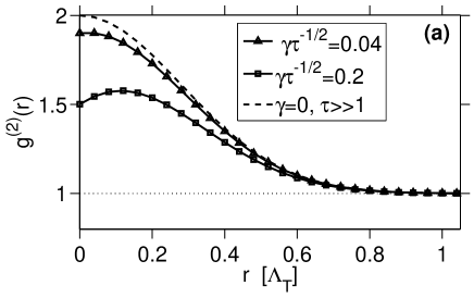
Together with (), this gives the following result for the pair correlation function in the DC regime ():
| (39) |
This is written in terms of the thermal de Broglie wavelength
| (40) |
a quantity that will appear repeatedly in what follows. At we have in agreement with Ref. karenprl . In the non-interacting limit () we recover the well-known result for the classical ideal gas Naraschewski-Glauber characterized by Gaussian decay with a correlation length . For we observe [see Fig. 1(a)] the emergence of anomalous behavior, with a global maximum at nonzero interparticle separation . This corresponds to the emergence of antibunching, , due to repulsive interactions. As is increased further, there is a continuous transition from the DC regime to the regime of high-temperature “fermionization” (see Sec. VI.2), with reducing further and the maximum moving to larger distances.
IV.3 Decoherent quantum regime
For temperatures below quantum degeneracy, with , only contributes to the Green’s function
| (41) |
which gives the relation between the density and the chemical potential , . Performing the Fourier transform of Eq. (41) one obtains the one-particle density matrix for the ideal gas
| (42) |
which characterizes the decay of phase coherence over a length scale given by
| (43) |
and also determines the second-order correlation function for the ideal gas
| (44) |
The one-particle Greens function, Eq. (41), together with Eq. (33) leads to . Inserting it into Eq. (32) we obtain (see Appendix B) corrections to , leading to the following result for the pair correlation function in the DQ regime
| (45) |
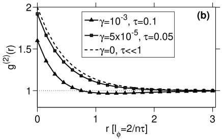
This has the maximum value , in agreement with the result of Ref. karenprl . For the correlations decay exponentially with the characteristic correlation length of half a phase coherence length describing the long-wavelength phase fluctuations.
An interesting feature in this regime is the apparent prediction of weak antibunching at a distance as seen in Fig. 1 (b), with . The strongest antibunching in expression (45) occurs at , or , and dips below unity by an amount . However, there is ambiguity regarding its existence: One should note that the dip below unity is very small in the region of uncontested validity of Eq. (45) where , and only becomes appreciable around , which is in the crossover region into the quasi-condensate (see Sec. V). Whether such anomalous antibunching survives higher order corrections in the small parameter remains to be seen. Our numerical calculations to date have not been able to access a regime of small enough to confirm or deny its existence.
IV.4 Quantum/classical transition
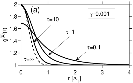
The transition from the quantum to the classical decoherent gas was investigated using the gauge- numerical method. The behavior is shown in Figs. 2–5.
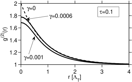
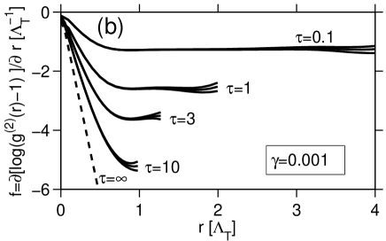
With rising temperature, still below degeneracy, one first finds a rounding-off of the exponential behavior at short ranges of a fraction of , as seen in Fig. 2. There is also a global lowering of with . It should be noted that the parameters for the numerical results shown in Fig. 2 are not deep in the regime where (45) applies accurately, and the lowering of the tails with is weaker here, than predicted by that limiting expression.
Considering variation with , as temperature approaches, and then exceeds , Gaussian thermal-like behavior appears first at short ranges, progressively taking over an ever larger part of as temperature is raised. This is seen in Fig. 3. The exponential tails can persist at ranges well into the high temperature regime when is small, as seen in Fig. 3(b) for and even .
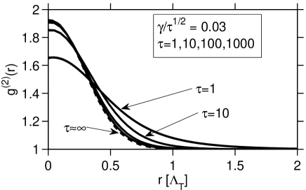
There are three scenarios that can typically be controlled in ultracold gas experiments: (i) varying the absolute temperature changes but not , as in Fig. 3; (ii) varying the coupling strength via a Feshbach resonance or varying the width of the trapping potential affects but not , as considered in Section VII and Fig. 2; and (iii) varying the linear density gives changes in both and , while keeping the quantity constant. Notably, this is the parameter that appears in the analytic expressions for both decoherent regimes, Eqs. (45) and (39).
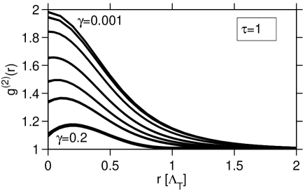
Figure 4 shows the behavior under scenario (iii), where increasing corresponds to decreasing density of the gas. As expected, tends to a constant value with predicted by Eq. (39). Interestingly, the crossover is quite broad under changing density, with departures from the decoherent classical result still visible at .
Finally, in the middle of the crossover region at , , there is the smooth and quite broad transition from low values of to that is shown in Fig. 5. The situation of a short-range Gaussian with standard deviation and exponential tails with length scale that was seen in Fig. 3 morphs into an anomalous form with a local maximum that is similar to the high temperature fermionization behavior described below in Sections VI and VII.
V Weakly interacting quasi-condensate regime []
In the regime of weak interactions and low temperature (or Gross-Pitaevskii regime) with we rely on the fact that the equilibrium state of the gas is that of a quasi-condensate mermin-wagner-hohenberg ; petrov-1d-regimes . In this regime the density fluctuations are suppressed while the phase still fluctuates. The pair correlation function is close to one and the deviations can be calculated using the Bogoliubov theory. In this approach, the field operator is represented as a sum of the (-number) macroscopic component , containing excitations with momenta (where is the healing length) and a small operator component describing excitations with larger momenta, . The momentum is chosen such that most of the particles are contained in , however, its details do not enter into the lowest order corrections to , which are . Using Wick’s theorem, and the property of the thermal density matrix that , the pair correlation function is then reduced to
| (46) |
The normal and anomalous averages and are calculated using the Bogoliubov transformation
| (47) |
where is the length of the quantization box, and are the annihilation and creation operators of elementary excitations, and are the expansion coefficients given by
| (48) |
and satisfying . Here is the Bogoliubov excitation energy, , and we note that the following useful relationships between and hold:
| (49) | |||||
| (50) |
where is the healing length. The equilibrium occupation numbers of the Bogoliubov excitations are given by .
Applying the Bogoliubov transformation to the normal and anomalous averages in Eq. (46) gives
| (51) | |||||
Using next Eq. (48) for the coefficients and we obtain the following result for the pair correlation function
| (52) |
For convenience, we split the -function into two parts corresponding to the contributions of thermal and vacuum fluctuations,
| (53) |
with
| (54) |
and
| (55) |
We first evaluate the vacuum contribution , Eq. (54). As shown in Appendix C, the integral in (54) can be obtained exactly in terms of special functions, giving
| (56) |
where is the modified Struve function and is a Bessel function. The correlation length scale here is set by the healing length .
V.1 Quasi-condensate at low temperatures
At very low temperatures when the excitations are dominated by vacuum fluctuations, whereas the thermal fluctuations are a small correction, the -term is calculated as follows. First, we substitute the explicit expression for into Eq. (55), giving
| (57) |
As shown in Appendix C, for (or ) the integral can be simplified and gives
| (58) |
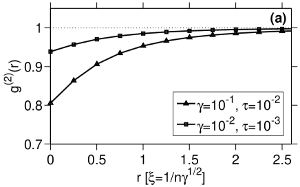
Combining Eqs. (53), (56) and (58) we obtain the following final result for this regime ():
| (59) |
In the limit of , the terms in the second line of Eq. (59) cancel each other and the large distance () asymptotics of the difference of special functions ensures the expected inverse square decay of correlationsgiamarchi-book . At small but finite temperatures, the same large-distance asymptotics exactly cancels the inverse square behavior in the second line of Eq. (59) leaving only the exponential decay
| (60) |
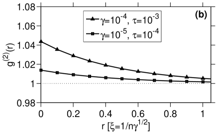
to the uncorrelated value of . This is again in full agreement with the Luttinger liquid theory giamarchi-book . We note that even at , oscillating terms are absent, in contrast to the strongly interacting regime of Sec. VI.3, Eq. (71). The limit in Eq. (59) reproduces the result of Eq. (9) of Ref. karenprl , . In Fig. 6(a) we plot Eq. (59) for different values of the interaction parameter , and we note that the finite temperature correction term is negligible here.
V.2 Thermally excited quasi-condensate
In the opposite limit, dominated by thermal rather than vacuum fluctuations and corresponding to , the thermal part of the pair correlation function is calculated as follows. We first note that large thermal fluctuations correspond to , which in turn requires . Thus, we replace in the integral (55) by . With this substitution, the integral for is dominated by the free-particle (quadratic in ) part of the Bogoliubov spectrum and the calculations in Appendix C yield
| (61) |
This result is valid for . For the main contribution to the integral in Eq. (55) comes from the phonon (linear in ) part of the Bogoliubov spectrum and one recovers the behavior given by Eq. (60).
Combining Eqs. (53), (56) and (61) we obtain the following final result for this regime ( and ):
| (62) |
The last two terms are due to vacuum fluctuations and are a negligible correction here, so the leading term gives an exponential decay of correlations [see Fig. 6(b)] with a characteristic correlation length given by the healing length . The peak value at is , in agreement with Ref. karenprl .
VI Strongly interacting regime []
VI.1 Perturbation theory in
By mapping the system onto that of a weakly attractive 1D fermion gas Cheon-Shigevare one can perform perturbation theory in . The formalism is the same as in Sec. IV.1, except that is now a fermionic field and the interaction term in the Hamiltonian (2) has to be modified to describe effective attractive interaction between fermions with matrix elements (in -space) Cheon-Shigevare . Then
with . The first order corrections to are given by the Hartree-Fock approximation as a sum of the direct and exchange contributions
| (63) | ||||
| (64) |
where
| (65) |
in terms of the Green’s function for free fermions.
VI.2 Regime of high-temperature “fermionization”
We proceed with evaluation in the regime of high-temperature “fermionization” at temperatures well above quantum degeneracy, . In this regime, we use the Maxwell-Boltzmann distribution of quasi-momenta as the unperturbed state. In the temperature interval , the characteristic distance related to the interaction between the particles – the 1D scattering length – is much smaller than the thermal de Broglie wavelength , and the small perturbation parameter is karenprl .
>From the same formalism as in Sec. IV.1, the free fermion Green’s function is now given by
| (66) |
so the integral for , Eq. (65), gives
| (67) |
The only effect of the exchange contribution is to cancel the delta-function in the direct contribution. This leaves us with the following result for the pair correlation function in the regime of high-temperature fermionization ():
| (70) |
In the limit this leads to perfect antibunching, , while the small finite corrections (as in Ref. karenprl , ) are reproduced at order . The correlation length associated with the Gaussian decay of correlations in Eq. (70) is given by thermal de Broglie wavelength . For not very large , the correlations do not decay in a simple way, but instead show an anomalous, non-monotonic behavior with a global maximum at at . This originates from the effective Pauli-like blocking at short range and thermal bunching [] at long range. As is increased the position of the maximum diverges and its value approaches 1 in a non-analytical way .
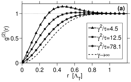
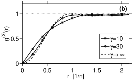
Figure 7(a) shows a plot of Eq. (70) for various ratios of . For a well-pronounced global maximum, moderate values of are required (such as , with , ), and these lie near the boundary of validity () for our perturbative result in the high-temperature fermionization regime. Exact numerical calculations described in Ref. drummond-canonical-gauge , and in more detail below in Sec. VII do, however, show qualitatively similar global maxima.
VI.3 Zero- and low-temperature (Tonks-Girardeau) regime
At the procedure is straightforward cherny_brand2 and yields the known korepin-book ; cherny_brand2 result
| (71) |
where . The last term here diverges logarithmically with and can be regarded as a first order perturbation correction to the fermionic inverse square power law. Accordingly, Eq. (71) is valid for .
At temperatures well below quantum degeneracy, , finite temperature corrections to Eq. (71) are obtained using a Sommerfeld expansion around the zero temperature Fermi-Dirac distribution for the quasi-momenta. For this gives an additional contribution of to the right hand side of Eq. (71), which is negligible compared to the result as . At , Eq. (71) gives perfect antibunching , which corresponds to a fully “fermionized” 1D Bose gas, where the strong inter-atomic repulsion mimics the Pauli exclusion principle for intrinsic fermions. By extending the perturbation theory to include terms of order we can reproduce the known result for the local pair correlation at zero temperature karenprl ; gangardt-correlations .
In Fig. 7(b) we plot the function , Eq. (71), for various . According to the physical interpretation of the pair correlation function , its oscillatory structure, and hence the existence of local maxima and minima at certain finite values of , implies that there exist more and less likely separations between the pairs of particles in the gas. This can be interpreted as a quasi-crystalline order (with a period of ) in the two-particle sector of the many-body wave function even though the density of the gas is uniform.
The oscillatory behavior of the pair correlation in this strongly interacting regime is similar to Friedel oscillations in the density profile of a 1D interacting electron gas with an impurity Friedel . We also mention that our derivation of Eq. (71) is equally valid for strong attractive interactions, i.e., when and , and therefore it describes the pair correlations in a metastable state known as super-Tonks gas super-Tonks .
VI.4 Numerical results
Numerical calculations with the gauge- method are able to reach only the low- (or, equivalently, high ) edge of the high-temperature fermionization regime, however a comparison with Eq. (70) is instructive. In Fig. 8 we see that the length scale on which antibunching occurs is still qualitatively given by Eq. (70) while any discrepancies are of the same size as at . This is actually a general feature in all the parameter regimes explored by the numerics. Overall, the discrepancy between the perturbation expansions (39), (45), (70), and the exact behavior of at nonzero is roughly the same as at . Since a calculation of karenprl from the exact solution of the Yang-Yang integral equations yangyang1 is usually more straightforward to evaluate than the full stochastic calculation of , it can serve as a useful guide to whether a numerical calculation is warranted or not.
VII Classical/Fermionization transition and correlation maxima
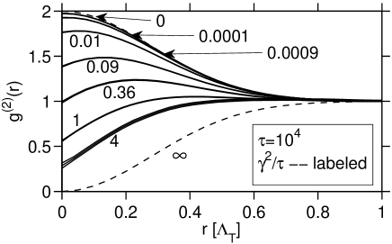
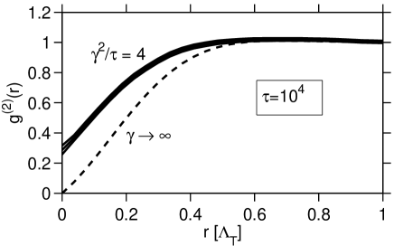
Figure 9 shows the behavior in the transition region between the decoherent classical and high temperature fermionization regimes (found with the gauge- numerical method), when one is far above the degeneracy temperature . One sees the appearance of a maximum in the correlations at finite range as the transition is approached. As pointed out in Sec. VI.2, this arises from an interplay of thermal bunching and repulsive antibunching on comparable scales. A comparison of relevant length scales indicates that the here corresponds to , where is the “1D scattering length” that describes the asymptotic behavior of the wave function in two-body scattering.
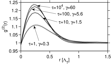
An interesting behavior occurs in the crossover regime when . Here we can have just like in the quasi-condensate or “Gross-Pitaevskii” regime, indicating local second-order coherence. However, unlike the quasi-condensate regime, the non-local correlations on length scales of are not coherent, and in fact appreciably bunched. This is shown in Fig. 10. It is a symptom of the broader correlation maximum phenomenon.
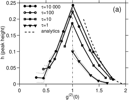
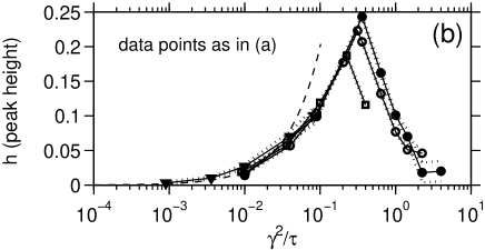
The height of this maximum for more general parameters is shown in Fig. 11 as a function of both and . One sees that this behavior is well pronounced in the crossover between high temperature fermionization and decoherent classical regimes, peaking when (a situation shown also in Fig. 10), or, equivalently, . As one reaches degenerate temperatures, the maximum peak height is reduced, and presumably disappears completely by the time the quasi-condensate regime is reached by going to smaller values of . Although we were unable to numerically reach the relevant quasi-condensate region for , a more refined numerical setup that improves the importance sampling or the trajectory described in Appendix A may allow this.
VIII Numerical limitations
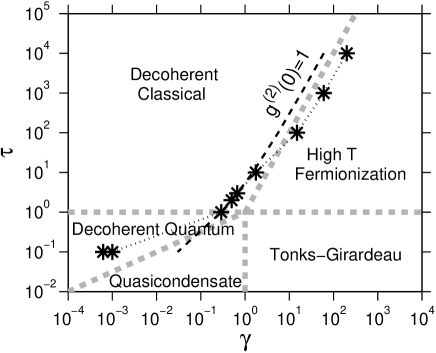
Figure 12 shows the regime that was accessible using the relatively straightforward numerical scheme that was employed here, and detailed in Appendix A. (It is the region above and to the left of the asterisks). In particular, one sees that of the physical regimes described in previous sections, the decoherent classical, as well as parts of the decoherent quantum and high-temperature fermionization regimes were accessible, while the quasi-condensate and Tonks-Girardeau regimes were not.
The principal difficulty that is encountered, generally speaking, is the growth of statistical noise with increasing , i.e. decreasing , which eventually prevents one from obtaining values of with a useful resolution. This arises in two different ways depending on the region of interest.
Firstly, in the strongly interacting (fermionized) region, one needs a correspondingly large coupling constant which leads to a relative increase of the importance of the noise terms of the equations in (21). This leads to large statistical uncertainty in the themselves or to the weight whose evolution depends on them. The upshot is that the inverse temperature at which the noise becomes unmanageable becomes smaller and smaller as grows. Technical improvements are unlikely to make a large dent in the problem in the fermionized regime because it ultimately stems from the fact that coherent states are no longer a good basis over which to expand the density matrix. They are not close to the preferred eigenstates of the system. Instead, one can think of constructing a phase-space distribution that uses a non-coherent-state basis, for example, a Gaussian basis CorneyDrummond . This general approach - together with symmetry projections - has been utilized in successfully calculating ground state properties of the strongly correlated fermionic Hubbard model AimiImada .
Secondly, in the low and region, one has a different underlying source of statistical uncertainty. The longest relevant length here is either the coherence length or the healing length , and for correct calculations in the large uniform gas one must simulate a system of a total size appreciably greater than these lengths. This in turn imposes a minimal total particle number
| (72) |
The thermal initial conditions of Eq. (12) lead to variation in among trajectories, and since the Gibbs factor (see Eq. (16) ) grows linearly or faster with , one also obtains a growing variation of . This enters the of Eq. (21) and leads to a spread of the weights that grows rapidly (note the exponential growth of ) with increasing . However because of the long length scales, via (72), large is needed to make accurate calculations when or are much smaller than one. The end result is domination of the whole calculation by one or a few trajectories with the highest weight, for all realistic ensemble sizes .
As a corollary, significantly lower temperatures, even down to the quasi-condensate regime, are accessible at small if one is prepared to sacrifice the assumption of an infinite-sized gas and consider periodic boundary conditions on some length that is smaller than or comparable to the coherence/healing lengths. This approach was taken, e.g., in Carusotto . This stops the rise of overall particle number, hence one has a much smaller spread of Gibbs factors among the trajectories, and in the final analysis – reduced statistical uncertainty. Such calculations are no longer as general, though, and are not considered in this paper.
We would like to point out that the limitation in this regime may be overcome or alleviated if the rather simplistic importance sampling used in the numerical method were to be improved. The leading candidate is an improved importance sampling algorithm, possibly using a Metropolis sampling procedure, as outlined at the end of Appendix A.3.
Finally, it is also possible that a more refined choice of (considered in Appendix A.5) may lead to somewhat improved coverage of the parameter space in general.
IX Overview and conclusion
In conclusion, we have surveyed the behavior of the spatial two-particle correlation function in a repulsive uniform 1D Bose gas. We have analyzed numerically the pair correlation functions for all relevant length scales, with the exception of several low-temperature transition regions (see Fig. 12 below the asterisks) which were not accessible by the numerical scheme we employed. Approximate analytic results and methods have been presented for parameters deep within all the major physical regimes. The key features of this behavior include:
-
•
Thermal bunching with and Gaussian drop-off at ranges in the classical decoherent regime.
-
•
Exponential drop-off of correlations from at ranges in the decoherent quantum regime, along with Gaussian-like rounding at shorter ranges .
-
•
Suppressed density fluctuations with and exponential decay at ranges of the healing length in the quasi-condensate regime.
-
•
Antibunching with and Gaussian decay at ranges in the high-temperature fermionization regime.
-
•
Antibunching with and oscillatory decay on ranges of the mean interparticle separation in the Tonks-Girardeau regime.
-
•
Bunching at a range of in the crossover between classical and fermionized regimes around .
Let us consider the regimes in turn, starting from the classical decoherent gas, then going anti-clockwise in Fig. 12. The classical decoherent gas is well approximated by Boltzmann statistics and is dominated by thermal fluctuations. The pair correlation function shows typical thermal bunching and a Gaussian decay, with the correlation length given by the thermal de Broglie wavelength .
As one reduces the temperature, the gas becomes degenerate, the thermal de Broglie wavelength becomes larger than the mean interparticle separation and loses its relevance. The correlation length increases and one enters into the decoherent quantum regime. Here, the dominant behavior of the gas is the ideal Bose gas bunching, , with large density fluctuations that decay exponentially on the length scale given by the phase coherence length . Notably, the exponential behaviour starts to appear well above degeneracy first in the long-distance tails, being visible even around as in Fig. 3.
Reducing the temperature even further, while still at , one enters into the quasi-condensate regime, in which the density fluctuations become suppressed and . In the hotter sub-regime dominated by thermal fluctuations, the pair correlation shows weak bunching, , while in the colder sub-regime dominated by quantum fluctuations one has weak antibunching, . In both cases the pair correlation decays on the length scale of the healing length .
We now move to the right on Fig. 12, into the regime of strong interactions, while staying at temperatures well below quantum degeneracy, . This is the Tonks-Girardeau regime, in which the density fluctuations get further suppressed due to strong interparticle repulsion. Antibunching increases and one approaches due to fermionization. The only relevant length scale here is the mean interparticle separation, , and the pair correlation function decays on this length scale with some oscillations.
We next move up on Fig. 12, to higher temperatures, and enter the regime of high-temperature fermionization. At short range, the pair correlation here is still antibunched due to strong interparticle repulsion, however, thermal effects start to show up on the length scale of . As a result of these competing effects, the nonlocal pair correlation develops an anomalous peak, corresponding to bunching at-a-distance, with , beginning around .
As we increase the temperature even further, the thermal effects start to dominate over interactions and the antibunching dip gradually disappears. At temperatures we observe a crossover back to the classical decoherent regime.
Our results provide new insights into the fundamental understanding of the 1D Bose gas model through many-body correlations. Calculation of these non-local correlations is not accessible yet through the exact Bethe ansatz solutions. We expect that our theoretical predictions will serve as guidelines for future experiments aimed at the measurement of nonlocal pair correlations in quasi-1D Bose gases.
Acknowledgements.
AGS, MJD, PDD and KVK acknowledge fruitful discussions with A. Yu. Cherny and J. Brand, and the support of this work by the Australian Research Council. DMG acknowledges support by EPSRC Advanced Fellowship EP/D072514/1. PD was supported by the European Community under the contract MEIF-CT-2006-041390. KVK, PD and DMG thank IFRAF and the Institut Henri Poincare–Centre Emile Borel for support during the 2007 Quantum Gases workshop in Paris where part of this work was completed. LPTMS is a mixed research unit No. 8626 of CNRS and Université Paris-Sud.Appendix A Technical appendix for the gauge- calculations
A.1 Instability of the stochastic equations and its removal with a stochastic gauge
A straightforward application of the ungauged diffusion Eqs. (19) is foiled by the presence of an instability in the equations. We can see this if we first consider the evolution of and discard the noise and kinetic-energy parts of the equation. Taking the deterministic part from the Stratonovich calculus which is used for our numerics (this introduces the term below), one has
| (73) |
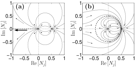
There are stationary points at the vacuum and at , with the more positive stationary point (usually ) being an attractor, and the more negative a repellor [see Fig. 13 (a) ]. The deterministic evolution is easily solved, and starting from a time gives later evolution as
| (74) |
If has a negative , which is possible due to the action of the noises , then at a later time
| (75) |
the solution has diverged to negative infinity. This behavior of the deterministic part of the equations is known as a “moving singularity” and is a well-known indicator of non-vanishing boundary terms when an integration-by-parts is performed on the operator equation (III.2) Gilchrist ; deuar-thesis . It implies that the FPE (18) is not fully equivalent to quantum mechanics.
The use of a stochastic gauge to remove this kind of instability has been described in deuar-drummond-2006 , and in more detail in deuar-thesis . The gauge identity, Eq. (17), can be used on Eq. (III.2) to introduce an arbitrary modification to the deterministic evolution (arising from first order derivative terms) for the price of additional diffusion in the weight . Since the gauge identity is zero, we can add an arbitrary multiple of it to Eq. (III.2). In particular, if we add
with arbitrary functions , and perform the subsequent steps as before, then the diffusion matrix in the resulting FPE remains positive semidefinite (no negative eigenvalues), and the resulting Ito diffusion equations of the samples become
| (77) | |||||
instead of (19). The equations are modified and compensating correlated noises have been added to the equation.
We now wish to choose the functions , called stochastic gauges, so that the instability is removed, keeping also in mind the goal of keeping the (now unbiased) statistical uncertainty manageable. Heuristic guidelines for choosing gauges have been investigated in detail in deuar-thesis . Several choices for a single-mode system were also investigated there in Sec. in terms of resulting statistical uncertainties. The aim is to remove the real part of from the equation when it is negative, so as to neutralize the moving singularity. While for a single mode the “radial” gauge was found to give the best performance, later tests that we have performed on the full multimode () 1D gas show that the “minimal” drift gauge
| (78) |
gives better performance for this system. This is because it introduces the smallest modifications needed to remove the moving singularity, and hence the smallest noise contributions to the weight . The weight becomes much more important for multimode systems because each of the modes adds its own contribution to it, the total of which can become large. The phase-space modification for a single mode for the ungauged Eq. (73) and gauged equations is shown in Fig. 13. One sees that in the “classical” region the trajectories are practically unchanged. The final Ito equations to be integrated are (21). Comparisons to known exact results such as energy and density yangyang1 , and karenprl indicate no deviations beyond what is predicted by the unbiased statistical uncertainties, Eq. (26), with the new gauged equations. Such a comparison can be seen in Fig. 2 of Ref. drummond-canonical-gauge .
A.2 Integration procedure
The actual integration is performed using a split-step semi-implicit method described in Ian , which requires the use of the Stratonovich stochastic calculus. There, it was shown to be highly superior to other low-order methods in terms of stability. Although a low order Newton-like method, with the right choice of variables its performance is remarkably good. High-order methods such as Runge-Kutta or others suffer from serious complications when noise is present. In particular, one has to be very meticulous in tracking down and compensating for all the non-zero correlations within a single time-step — these are much more complicated than the simplest correction terms appearing in the Stratonovich semi-implicit method used here.
Due to the multiplicative form of the equations (21), it is highly advantageous to use logarithmic variables, which is made possible if one uses a split-step method. Here, a timestep consists of the following four stages: First the interaction part (containing ) is integrated in real space over a time-step . Second, the fields are Fourier-transformed to -space, giving . Thirdly the kinetic-energy contributions are integrated over , and finally one Fourier-transforms back into real space, ready to start the next timestep. The Stratonovich gauged evolution equations for the real space stage are
| while for the -space stage they are | |||||
| (79b) | |||||
A.3 Importance sampling
The simulated equations (21) include evolution of both the amplitudes and weight . This combination can cause sampling problems for observable estimations, Eq. (22), when maximum weights occur for very rare trajectories. As it turns out, this was a serious issue for the majority of calculations reported here because while the initial distribution (12) samples the system well, this is not necessarily the case during the later evolution into that is of most interest. Fortunately, fairly rudimentary importance sampling was able to deal with this for a wide range of parameters.
The essence of this approach is to pre-weight trajectories in such a way that the part of the distribution with maximum weight coincides with the majority of samples at the target time of interest , rather than at . The price paid is that the distribution is then poorly sampled, but this is not important to us as we are interested rather in the target .
Pre-weighting is made possible because in all observable calculations (22), the combination occurs as a universal common factor in the integral. Hence, if we manually scale the weight by some factor of our choice: , and simultaneously rescale the distribution according to , then with and one obtains exactly the same results in the infinite-number-of-samples limit as with . However, the actual samples are differently distributed, which is advantageous for finite sample numbers. To reduce the weight sampling problem, one wants to make such a modification that both and peak in the same region of the phase space of .
To proceed, it is convenient to consider Fourier-transformed variables in -space, where the non-interacting evolution can be easily exactly solved. Define then
| (80) |
where takes on discrete values from to . The “naive” initial distribution (12) then becomes
| (81) |
This is a thermal distribution which is uniform over all . The ideal gas (i.e. ) evolution of equations (21) then leads to
| (82) | |||||
where
| (83) |
with being independent complex Gaussian noises with variance unity, . One can see that (82) is not necessarily anywhere near a well-sampled ideal gas Bose-Einstein distribution at temperature , which would have
| (84) |
with
being the usual Bose-Einstein distribution.
For the purpose of the simulations presented here, a fairly crude yet effective importance sampling was applied as follows. For relatively weak coupling , a very rough but useful estimate of the thermal state at coarse resolution is that the Fourier modes are decoupled and thermally distributed with some mean occupations at the target time that we are interested in. In practice we will choose some estimate of the guiding density . The desired equal weight sampling at time would then correspond to the distribution
| (85) | |||||
which leads to samples given by and . What we are interested in is the corresponding distribution of samples at . An estimate of the initial distribution that leads to can be obtained by evolving (85) back in imaginary time using only kinetic interactions. This is again rather rough, since deterministic interaction terms are omitted, not to mention noise, but it is simple to carry out and proved sufficient for our purposes here. One obtains then an estimated sampling distribution for samples at :
| (86) | |||||
where
| (87) |
and the pre-weight now depends on the set of particular values of at obtained for a given sample, according to
| (88) |
For most of the simulations reported here, taking to be just the ideal gas Bose-Einstein distribution was sufficient. However, once the chemical potential approaches or exceeds zero, this estimate is no longer useful. A better choice for is the density of states function of the exact Yang and Yang solution yangyang1 , although it should be noted that this is not the density of actual particles that we seek. In practice, our approach was to first run a calculation based on this estimate , obtain a better estimate of the real density from this full stochastic calculation by evaluating the expectation value of using Eq. (22), then finally use this expectation value to choose an improved preweighting function for a “second-generation” calculation.
One important point to make regarding the choice of is that one should endeavor always to choose the preweighting guide density equal or greater than the real density, never smaller. The reasoning behind this is as follows: Suppose first one chooses a guiding function that is much smaller than the true k-space density . This means that the variance of the samples will be too small to recover the physical value of the density upon averaging without resorting to very large weights for the largest samples. In practice, if the ratio is small, then the typical trade-off that occurs is that the largest contribution to comes from those that are many standard deviations from the mean. Their rarity is compensated for by a very large . However, this is fatal for practical numbers of samples because in fact not even one of the samples one obtains ends up in this highest-contribution region at many standard deviations from the mean. For , the number of samples with will be , i.e. vanishing, leading to a systematic error.
In contrast, the opposite situation when is chosen too large is much more benign. Following the above reasoning, one gets a distribution of samples that is too broad, with the result that a majority of samples are too far away from physical values of and their excessive abundance must be compensated for by giving them a correspondingly small weight. However, for reasonably large numbers of trajectories, there always remains a core of the smallest samples that are in the region of most important contributions. The number of these samples is of the order of , which is reasonable in practice as long as the estimate is not extremely poor.
Finally, it should be mentioned that superior importance sampling schemes to the crude one we have employed here could be implemented and may allow one to reach much lower temperatures than presented here. A first step would be to keep the distribution estimate, Eq. (85), but estimate the resulting initial samples at in a more accurate manner. To do this, one could choose the samples according to and as usual, but then evolve them back in time to numerically, using the deterministic part of the full equations (21). This would give a superior estimate of the initial distribution as it takes into account mean field effects as well as kinetic evolution. Having these samples, one would then proceed forward in time with the full stochastic evolution.
A further refinement would be to choose initial samples via the Metropolis algorithm, so that the initial samples are distributed according to , where when is calculated according to the deterministic part of the evolution, Eq. (21), starting from . This avoids the arbitrariness of the crude Gaussian choice, Eq. (85). A final, but numerically intensive approach would be to sample the phase-space variables and directly via a Monte Carlo Metropolis algorithm whose free parameters to be varied include both the initial noises and all the time-dependent noises for a given time lattice .
A.4 Trust indicators for sampling
One should mention two heuristic trust indicators that we use extensively to exclude bad sampling of the underlying phase-space distribution.
Firstly, let us point out that the behavior of the evolution equations (79) is such that one builds up an approximately Gaussian distribution of the logarithmic variables (leaving aside the evolution of itself, which is initially small). This means that the stochastic averages to be evaluated, e.g., in Eq. (25), involve means of exponentials of approximately Gaussian random variables (as per with Gaussian). A feature of such means is that if the variance of the logarithm exceeds a value of around the mean begins to have systematic error when calculated with any practical sample sizes. This is discussed in detail in deuar-drummond-pp ; deuar-thesis . As a result, when calculating observables with some expression , one must also check that the variance of its logarithm is small enough, i.e. that
| (89) |
If this is not satisfied, the results for must be considered suspect.
Secondly, sampling problems of this sort usually make themselves visible if one compares two calculations with widely different sample sizes. In practice one can evaluate an average and its uncertainty with samples, and with samples (where, of course, ). If the difference is statistically significant the result of the sample average again should be considered suspect.
A.5 Choice of intermediate
If one is primarily interested in the behavior of the system around some target temperature and chemical potential (alternatively – density), then the values of at intermediate times can in principle be chosen at will.
In practice, however, some choices lead to smaller statistical uncertainty than others because the intermediate values of density affect the amount of noise generated during the evolution. A preliminary investigation of choice in deuar-thesis indicated some heuristic guidelines that were also followed in the present work:
(i) It is advantageous to not vary too much over the course of the simulation. Excessive variation leads to increased noise.
(ii) A constant or piecewise-constant value of is also advantageous because the ideal-gas part of the evolution can then be calculated exactly in logarithmic variables (79b), and step-size is only important for the interaction part of the evolution.
(iii) It is advantageous to choose an initial density that is much smaller than the final one at both for statistical sampling reasons and because this puts the initial gas much further into the classical decoherent regime (), where the initial condition (12) applies, than the final regime.
In practice, our simulations used the following form
| (90) |
which is piecewise constant over a time step , with the fugacity
| (91) |
Here, and are the target inverse temperature and fugacity, and and are numerical constants for the initial high temperature state that we chose to be and .
Given the difficulty of precisely analyzing the statistical behavior, it is unclear whether a wiser choice of may lead to significant improvements over the results presented here. However, this is the most successful choice of those we tried.
Appendix B Integrals in perturbation theory in
We begin with Eq. (32) and substitute the expression for in Eq. (37) to give
| (92) |
Next we make the substitution and to give
| (93) | |||||
| (94) |
where the last equality follows from the substitution . The exponent in the integrand of Eq. (94) can be represented as a Gaussian integral
| (95) |
Then, changing the order of integration in Eq. (94) we arrive at
| (96) | |||||
The final result shown in Eq. (38) follows trivially from a shift in the integration variable , and the definition of the complimentary error function,
| (97) |
Appendix C Integrals in the Bogoliubov treatment
We first evaluate the vacuum contribution , Eq. (54). Writing down the integral explicitly, in terms of , and transforming to a new variable , we have
| (98) |
Integrating by parts, gives
| (99) |
The integral in (99) can be expressed in terms of special functions MathHandbook , giving
| (100) |
The finite temperature term , Eq. (57), is evaluated by performing variable changes according to , followed by and then . In this way we transform the integral over to an integral over
| (101) |
where . So far we have not made any additional assumptions or approximations.
By inspecting the integrand in Eq. (101) one can see that for the main contribution to the integral comes from . Therefore for () we can simplify the integral by treating in the integrand as a small parameter. Accordingly, we obtain
| (102) | |||
| (103) |
and therefore
| (104) |
where we have introduced .
In the opposite limit, dominated by thermal fluctuations and corresponding to , we first note that large thermal fluctuations correspond to , which in turn requires . Thus, we replace in the integral (55) by . As a result, the thermal contribution becomes
| (106) |
which is valid for . Rewriting this in terms of the dimensionless parameters and we obtain Eq. (61). For the cosine term becomes important and the values of momenta in the integral Eq. (101) are cut off by . In this regime one can use the approximation that led to Eq. (105).
Appendix D Integrals in perturbation theory in
We begin by evaluating the direct contribution given by Eq. (63) by substituting Eq. (67),
| (107) | |||||
where we have affected the change of variables , and . The integration with respect to can then be done using integration by parts, which yields
| (108) | |||||
where the last equality follows from the substitution . The simplest way to solve the integral in Eq. (108) is by comparison with Eq. (93) in Appendix B. In doing so, one may observe
| (109) | |||||
| (110) |
The result shown in Eq. (68) then follows trivially from this.
In order to calculate the exchange contribution we begin with Eq. (64) and substitute Eq. (67), which immediately yields
| (111) |
where , and , and are defined the same was as for the direct contribution. The integration with respect to can be carried out using integration by parts, leaving an integral with respect to :
| (112) | |||||
where the first equality comes from the substitution and the second from . Both terms are standard definite integrals it is straightforward to show that
| (113) |
Thus the only effect of the exchange contribution is to cancel the delta-function contribution coming from the direct contribution at .
References
- (1) R. Hanbury Brown and R. Q. Twiss, Nature 177, 27 (1956).
- (2) M. Yasuda and F. Shimizu, Phys. Rev. Lett. 77, 3090 (1996).
- (3) M. Schellekens et al., Science 310, 648 (2005).
- (4) T. Jeltes et al., Nature 445, 402 (2007).
- (5) E. H. Lieb and W. Liniger, Phys. Rev. 130, 1605 (1963).
- (6) E. H. Lieb, Phys. Rev. 130, 1616 (1963).
- (7) C. N. Yang, C. P. Yang, J. Math. Phys. 10, 1115 (1969).
- (8) V. E. Korepin, N. M. Bogoliubov, and A. G. Izergin, Quantum Inverse Scattering Method and Correlation Functions (Cambridge University Press, 1993).
- (9) T. Giamarchi, Quantum Physics in One Dimension (Oxford University Press, 2004).
- (10) A. O. Gogolin, A. A. Nersesyan, and A. M. Tsvelik, Bosonization and Strongly Correlated Systems (Cambridge University Press, 2004).
- (11) M. D. Girardeau, J. Math. Phys. 1, 516 (1960); M. D. Girardeau, Phys. Rev. 139, B500 (1965); see also: L. Tonks, Physical Review 50, 955 (1936).
- (12) A. Görlitz et al., Phys. Rev. Lett. 87, 130402 (2001).
- (13) F. Schreck et al., Phys. Rev. Lett. 87, 080403 (2001).
- (14) M. Greiner, I. Bloch, O. Mandel, T. W. Hänsch, and T. Esslinger, Phys. Rev. Lett. 87, 160405 (2001).
- (15) M. Greiner, I. Bloch, O. Mandel, T. W. Hänsch, and T. Esslinger, Applied Physics B - Lasers and Optics 73, 769 (2001).
- (16) S. Richard et al., Phys. Rev. Lett. 91, 010405 (2003).
- (17) H. Moritz, T. Stöferle, M. Kohl, and T. Esslinger, Phys. Rev. Lett. 91, 250402 (2003).
- (18) B. Laburthe Tolra et al., Phys. Rev. Lett. 92, 190401 (2004).
- (19) B. Paredes et al, Nature (London) 429, 277 (2004).
- (20) T. Kinoshita, T. Wenger, and D. S. Weiss, Science 305, 1125 (2004).
- (21) T. Kinoshita, T. Wenger, and D. S. Weiss, Phys. Rev. Lett. 95, 190406 (2005).
- (22) T. Stöferle, H. Moritz, C. Schori, M. Kohl, and T. Esslinger, Phys. Rev. Lett. 92, 130403 (2004).
- (23) T. P. Meyrath, F. Schreck, J. L. Hanssen, C. S. Chuu, and M. G. Raizen, Phys. Rev. A 71, 041604(R) (2005).
- (24) J. Esteve et al., Phys. Rev. Lett. 96, 130403 (2006).
- (25) S. Hofferberth et al., Nature (London) 449, 324 (2007).
- (26) A. H. van Amerongen, J. J. P. van Es, P. Wicke, K. V. Kheruntsyan, and N. J. van Druten, Phys. Rev. Lett. 100, 090402 (2008)
- (27) Y. Castin et al., J. Mod. Opt. 47, 2671 (2000).
- (28) D. M. Gangardt and G. V. Shlyapnikov, Phys. Rev. Lett. 90, 010401 (2003).
- (29) D. M. Gangardt and G. V. Shlyapnikov, New J. Phys. 5, 79 (2003).
- (30) K.V. Kheruntsyan, D. M. Gangardt, P. D. Drummond, G. V. Shlyapnikov, Phys. Rev. Lett. 91, 040403 (2003).
- (31) M. A. Cazalilla, Phys. Rev. A 67, 053606 (2003); M. A. Cazalilla, New J. Phys. 37, S1 (2004).
- (32) K.V. Kheruntsyan, D. M. Gangardt, P. D. Drummond, G. V. Shlyapnikov, Phys. Rev. A 71, 053615 (2005).
- (33) G. E. Astrakharchik and S. Giorgini, Phys. Rev. A 68, 031602(R) (2003); G. E. Astrakharchik and S. Giorgini, J. Phys. B 39, S1 (2006).
- (34) P. D. Drummond, P. Deuar, and K. V. Kheruntsyan, Phys. Rev. Lett. 92, 040405 (2004).
- (35) A. Lenard, J. Math. Phys. 5, 930 (1964).
- (36) T. D. Schultz, J. Math. Phys. 4, 666 (1963).
- (37) J.-S. Caux and P. Calabrese, Phys. Rev. A 74, 031605(R) (2006).
- (38) J.-S. Caux, P. Calabrese, and N. A. Slavnov, J. Stat. Mech. P01008 (2007).
- (39) J. Brand and A. Yu. Cherny, Phys. Rev. A 72, 033619 (2005).
- (40) A. Yu. Cherny and J. Brand, Phys. Rev. A 73, 023612 (2006).
- (41) E. H. Lieb, R. Seiringer, J. P. Solovej, and J. Yngvason, arXiv:cond-mat/0610117v1 (unpublished).
- (42) D. S. Petrov, D. M. Gangardt, and G. V. Shlyapnikov, J. Phys. IV (France ) 116, 3 (2004).
- (43) Y. Castin, J. Phys. IV (France) 116, 89 (2004).
- (44) A. G. Sykes, D. M. Gangardt, M. J. Davis, K. Viering, M. G. Raizen, and K. V. Kheruntsyan, Phys. Rev. Lett. 100, 160406 (2008).
- (45) P. Deuar and P. D. Drummond, Phys. Rev. A 66, 033812 (2002).
- (46) P. D. Drummond and P. Deuar, J. Opt. B: Quantum Semiclass. Opt. 5, S281 (2003).
- (47) P. Deuar and P. D. Drummond, J. Phys. A: Math. Gen. 39, 2723 (2006).
- (48) P. Deuar, PhD thesis, The University of Queensland, eprint cond-mat/0507023.
- (49) T. C. Li et al., Opt. Express 16, 5465 (2008).
- (50) M. Olshanii, Phys. Rev. Lett. 81, 938 (1998).
- (51) I. Bouchoule, K. V. Kheruntsyan, and G. V. Shlyapnikov, Phys. Rev. A 75, 031606(R) (2007).
- (52) A. G. Sykes, P. D. Drummond, and M. J. Davis, Phys. Rev. A 76, 063620 (2007).
- (53) P. D. Drummond and C. W. Gardiner, J. Phys. A: Math. Gen. 13, 2353 (1980).
- (54) C. W. Gardiner, Quantum Noise (Springer-Verlag, Berlin, 1992).
- (55) A. Gilchrist, C. W. Gardiner, and P. D. Drummond, Phys. Rev. A 55, 3014 (1997).
- (56) Note that Eq. (30) only contains 4 terms coming from Wick’s theorem, the other 20 terms are disconnected corrections (in the language of Feynman diagrams) and hence only produce corrections to the single particle Green functions. That is they represent the interacting corrections to the relation between chemical potential and density.
- (57) M. Naraschewski and R. J. Glauber, Phys. Rev. A 59, 4595 (1999).
- (58) N. D. Mermin and H. Wagner, Phys. Rev. Lett. 17, 1133 (1966); P. C. Hohenberg, Phys. Rev. 158, 383 (1967).
- (59) D. S. Petrov, G. V. Shlyapnikov, and J. T. M. Walraven, Phys. Rev. Lett. 85, 3745 (2000).
- (60) T. Cheon and T. Shigehara, Phys. Rev. Lett. 82, 2536 (1999); D. Sen, J. Phys. A 36, 7517 (2003).
- (61) J. Friedel, Nuovo Cimento Suppl. 7, 287 (1958).
- (62) G. E. Astrakharchik, J. Boronat, J. Casulleras, and S. Giorgini, Phys. Rev. Lett. 95, 190407 (2005); M. Batchelor et al., J. Stat. Mech. L10001 (2005).
- (63) J. F. Corney and P. D. Drummond, Phys. Rev. Lett. 93, 260401 (2004).
- (64) T. Aimi and M. Imada, J. Phys. Soc. Japan 76, 084709 (2007); T. Aimi and M. Imada, J. Phys. Soc. Japan 76, 113708 (2007).
- (65) I. Carusotto, and Y. Castin, J. Phys. B: At. Mol. Opt. Phys. 34, 4589 (2001).
- (66) P. D. Drummond and I. K. Mortimer, J. Comput. Phys. 93, 144 (1991).
- (67) P. Deuar and P. D. Drummond, J. Phys. A: Math. Gen. 39, 1163 (2006).
- (68) Handbook of Mathematical Functions, Eds. M. Abramowitz and I. A. Stegun (Dover, New York, 1965).