Numerical solution and verification of the local equilibrium for the flat interface in the two-phase binary mixture.

Abstract

In this paper we first apply the general analysis described in our first paper to a binary mixture of cyclohexane and $n$-hexane. We use the square gradient model for the continuous description of a non-equilibrium surface and obtain numerical profiles of various thermodynamic quantities in various stationary state conditions. In the second part of this paper we focus on the verification of local equilibrium of the surface as described with excess quantities. We give a definition of the temperature and chemical potential difference for the surface and verify that these quantities are independent of the choice of the dividing surface. We verify that the non-equilibrium surface can be described in terms of Gibbs excess densities which are in good approximation equal to their equilibrium values at the temperature and chemical potential difference of the surface.

I Introduction

In a previous article glav/grad1 , referred to as paper I, we have established the general approach for the square gradient description of the interface between two phases in non-equilibrium mixtures. We considered phenomena like temperature, density and mass fraction gradients; heat and diffusion fluxes as well as evaporation or condensation fluxes through the interface. Some profiles were given, without going into details of the numerical procedures used to obtain them. In this paper we will do this.

In the general description of the interface one uses contributions to the Helmholtz free energy density proportional to the square of the density and mass fraction gradients. These contribution imply that it is not possible to use continuous local equilibrium thermodynamics in the interface, i.e. to calculate the local values of the various thermodynamic parameters in terms of the local density, mass fractions and temperature only. Rowlinson and Widom (see (RowlinsonWidom, , page 43)) use the name point thermodynamics for this to distinguish it from other quasi- or local thermodynamic treatments. Given the non-autonomous nature of the square gradient model, it is sensible to question whether a description in terms of excess variables along the lines given by Gibbs Gibbs/ScientificPapers , can be autonomous. Gibbs’ treatment, though only given for equilibrium systems, suggested such an assumption. This would imply that the surface is a separate thermodynamic phase. Bakker Bakker/capilarity and Guggenheim (Guggenheim/thermodynamics, , page 45) made this assumption, the validity of which was subsequently disputed by Defay and Prigogine DefayPrigogine/sta . We refer to Rowlinson and Widom (RowlinsonWidom, , page 33) for a discussion of this point. In the theory of non-equilibrium thermodynamics of surfaces bedeaux/boundaryNE ; bedeaux/advchemphys ; albano/electrosurf ; kjelstrupbedeaux/heterogeneous Gibbs’ description in terms of excess variables has been used. It is then assumed that the Gibbs’ description of the surface in terms of excess variables is autonomous, or in other words that one can use this property, which we will call local equilibrium of the surface, to describe the surface. In earlier work bedeaux/vdW/II coauthored by one of us this property was verified for one-component systems. It is the main objective of this paper to verify this property for binary mixtures. For details about the extension of the square gradient model to non-equilibrium systems we refer to paper I. For figures of typical density, mass fraction and temperature profiles, and a discussion thereof, we also refer to the first paper. In this paper we focus on the properties of the excess variables.

We consider a flat interface between a binary liquid and it’s vapor with the normal ${\mathbf{n}}=(1,0,0)$ pointing from the vapor to the liquid. We assume that all fluxes and gradients gradients are in the $x-$direction. Due to this all variables depend only on the $x-$coordinate. We assume the fluid to be non-viscous, so that the viscous pressure tensor $\pi_{\alpha\beta}=0$.

In Sec. [II] we will give all the equations, which are required for the determination of the profiles. We shall only consider stationary states in this paper. We choose the system such that the gas is on the left hand side and the liquid is on the right hand side. The $x$-axes is directed from left to right and the gravitational acceleration $g$ is directed towards the liquid. In Sec. [III] we describe numerical procedure which have been used to solve these equations. We give the results in Sec. [IV]. We then proceed to the second part of the article, the verification of local equilibrium of the surface. In Sec. [V] we introduce excesses and surface variables and discuss in general the meaning of local equilibrium of the surface. In Sec. [VI] we give the results of the verification procedure. Finally, in Sec. [VII] we give concluding remarks.

II Complete set of equations.

In order to calculate the various profiles in the non-equilibrium mixture a complete set of equations is required. This set is given by the hydrodynamic balance (conservation) equations, the thermodynamic equations of state and the phenomenological force-flux relations. These equations were given (derived) and discussed in paper I, to which we refer. In this paper we will only list them for the stationary case.

II.1 Conservation equations.

In a stationary state the conservation equations take the following form. The law of mass conservation is

$$\begin{array}[]{rl}\displaystyle{\frac{d}{dx}}\left(\rho\,{\rm{v}}\right)&=0\\ \\ \displaystyle{\frac{d}{dx}}\left(J_{1}+\rho\,\xi\,{\rm{v}}\right)&=0\end{array}$$ (II.1)

where $\rho=\rho_{1}+\rho_{2}$ and ${\rm{v}}=(\rho_{1}\,{\rm{v}}_{1}+\rho_{2}\,{\rm{v}}_{2})/\rho$ are the mass density and the barycentric velocity. Furthermore $\xi=\rho_{1}/\rho$ is the mass fraction of the first component and $J_{1}=\rho\,\xi\,({\rm{v}}_{1}-{\rm{v}})$ is the diffusion flux of the first component relative to the barycentric frame of reference. Momentum conservation is given by

$$\begin{array}[]{l}\displaystyle{\frac{d}{dx}}\left(\rho\,{\rm{v}}^{2}+p+\gamma_{xx}\right)=\rho\,g\end{array}$$ (II.2)

where we call $\gamma_{\alpha\beta}$ the thermodynamic tension tensor, which will be defined below. Furthermore $p$ and $p+\gamma_{xx}$ are the pressures parallel and perpendicular to the interface, for the planar interface under consideration. For curved surfaces see paper I. Energy conservation is given by

$$\begin{array}[]{l}\displaystyle{\frac{d}{dx}}\,J_{e}=0\end{array}$$ (II.3)

where $J_{e}\equiv J_{q}+\rho\,e\,{\rm{v}}+p\,{\rm{v}}$ is the total energy flux, $J_{q}$ is the heat flux, and $e=u+({\rm{v}}^{2}/2-g\,x)$ is the total specific energy and $u$ is the specific internal energy.

II.2 Thermodynamic equations.

The gradient model, discussed in the first paper glav/grad1 gives the following expressions for the specific Helmholtz energy $f$, the specific internal energy $u$, the parallel pressure $p$, the chemical potential difference $\psi\equiv\mu_{1}-\mu_{2}$, the chemical potential of the second component $\mu\equiv\mu_{2}$ and the $xx$-element of the tension tensor $\gamma_{xx}$:

$$\begin{array}[]{rl}f(x)&=f_{0}(T,\,\rho,\,\xi)+{\cal K}(\rho,\,\xi,\,\rho^{\prime},\,\xi^{\prime})\\ \\ u(x)&=f_{0}(T,\,\rho,\,\xi)-T\,\displaystyle\frac{\partial}{\partial T}f_{0}(T,\,\rho,\,\xi)+{\cal K}(\rho,\,\xi,\,\rho^{\prime},\,\xi^{\prime})\\ \\ p(x)&=\rho^{2}\displaystyle\frac{\partial}{\partial\rho}\left(f_{0}(T,\,\rho,\,\xi)+{\cal K}(\rho,\,\xi,\,\rho^{\prime},\,\xi^{\prime})\right)-\rho\,\displaystyle{\frac{d}{dx}}\left(\rho\,\displaystyle\frac{\partial}{\partial\rho^{\prime}}{\cal K}(\rho,\,\xi,\,\rho^{\prime},\,\xi^{\prime})\right)\\ \\ \psi(x)&=\displaystyle\frac{\partial}{\partial\xi}\left(f_{0}(T,\,\rho,\,\xi)+{\cal K}(\rho,\,\xi,\,\rho^{\prime},\,\xi^{\prime})\right)-{\frac{1}{\rho}}\,\displaystyle{\frac{d}{dx}}\left(\rho\,\displaystyle\frac{\partial}{\partial\xi^{\prime}}{\cal K}(\rho,\,\xi,\,\rho^{\prime},\,\xi^{\prime})\right)\\ \\ \mu(x)&=\displaystyle\frac{\partial}{\partial\rho}\left(\rho\,\left(f_{0}(T,\,\rho,\,\xi)+{\cal K}(\rho,\,\xi,\,\rho^{\prime},\,\xi^{\prime})\right)\right)-\psi(x)\,\xi-\rho\,\displaystyle{\frac{d}{dx}}\left(\rho\,\displaystyle\frac{\partial}{\partial\rho^{\prime}}{\cal K}(\rho,\,\xi,\,\rho^{\prime},\,\xi^{\prime})\right)\\ \\ \gamma_{xx}(x)&=2\,\rho\,{\cal K}(\rho,\,\xi,\,\rho^{\prime},\,\xi^{\prime})\\ \end{array}$$ (II.4)

Here $f_{0}(T,\,\rho,\,\xi)=f_{0}^{\nu}(T,\,c,\,\zeta)$ is the specific Helmholtz energy of the homogeneous phase, which can for instance be derived from the equation of state. Furthermore ${\cal K}(\rho,\,\xi,\,\rho^{\prime},\,\xi^{\prime})$ is the gradient contribution, where the primes indicate a derivative with respect to $x$. Since the equation of state is usually given in molar quantities, it is convenient to use them here as well. Thus, $c=\rho/M$ is the molar concentration, $\zeta=\xi\,M/M_{1}$ is the molar fraction, where $M=M_{1}\,M_{2}/(M_{1}+\xi\,(M_{2}-M_{1}))=M_{2}+\zeta\,(M_{1}-M_{2})$ is the molar mass of the mixture, and $M_{1}$ and $M_{2}$ are molar masses of each component.

II.3 The homogeneous Helmholtz energy

This energy is given by the following equation

$$f_{0}^{\nu}(T,\,c,\,\zeta)=-R\,T\,\ln\left({\frac{e}{c\,N_{A}}}{\frac{\mathrm{w}(T,\,\zeta)}{\Lambda^{3}(T,\,\zeta)}}\,\left(1-B(\zeta)\,c\right)\right)-A(T,\,\zeta)\,c$$ (II.5)

where the de Broglie wavelength $\Lambda$ and the characteristic sum over internal degrees of freedom w are respectively.

$$\begin{array}[]{l}\Lambda(T,\,\zeta)=\hbar N_{A}\displaystyle\left(\frac{2\pi}{MR\,T}\right)^{1/2}\\ \\ \mathrm{w}(T,\,\zeta)=\displaystyle\left(\frac{\mathrm{w}_{1}}{\zeta}\left({\frac{M_{1}}{M}}\right)^{\!3/2}\right)^{\zeta}\,\left(\frac{\mathrm{w}_{2}}{1-\zeta}\left({\frac{M_{2}}{M}}\right)^{\!3/2}\right)^{1-\zeta}\end{array}$$ (II.6)

Expressions for the characteristic sums over internal degrees of freedom for each component, $\mathrm{w}_{1}$ and $\mathrm{w}_{2}$, are given in paper I. In this paper they are assumed to be independent of the temperature and the molar fractions, i.e. just constant numbers.

The mixing rules for $A$ and $B$ are

$$\begin{array}[]{rcl}A(T,\,\zeta)&=&a_{11}\,\zeta^{2}+2\,a_{12}\,\zeta\,(1-\zeta)+a_{22}\,(1-\zeta)^{2}\\ B(\zeta)&=&b_{1}\,\zeta+b_{2}\,(1-\zeta)\end{array}$$ (II.7)

with $a_{ij}=\sqrt{a_{i}\,a_{j}}$, where $a_{i}$ as well as $b_{i}$ is a coefficient of a pure component $i$. We will assume in this paper that $a_{ij}$ are independent of temperature.

II.4 The gradient contribution

This contribution is given by the following general expression for a binary mixture

$$\begin{array}[]{l}{\cal K}(\rho,\,\xi,\,\rho^{\prime},\,\xi^{\prime})\equiv\displaystyle{\frac{1}{2\,\rho}}\left(\kappa_{\rho\rho}(\rho,\,\xi)\,{\rho^{\prime}}^{2}+2\,\kappa_{\rho\xi}(\rho,\,\xi)\,{\rho^{\prime}}\,{\xi^{\prime}}+\kappa_{\xi\xi}(\rho,\,\xi)\,{\xi^{\prime}}^{2}\right)\end{array}$$ (II.8)

The coefficients $\kappa_{\rho\rho}$, $\kappa_{\rho\xi}$ and $\kappa_{\xi\xi}$ can be expressed in the gradient coefficients $\kappa_{\rho_{1}\rho_{1}}$ and $\kappa_{\rho_{2}\rho_{2}}$ for components 1 and 2 in the following way (see paper I for details)

$$\begin{array}[]{rcl}\kappa_{\rho\rho}(\rho,\,\xi)&=&(\kappa_{\rho_{1}\rho_{1}}-2\kappa_{\rho_{1}\rho_{2}}+\kappa_{\rho_{2}\rho_{2}})\,\xi^{2}+2\,(\kappa_{\rho_{1}\rho_{2}}-\kappa_{\rho_{2}\rho_{2}})\,\xi+\kappa_{\rho_{2}\rho_{2}}\\ \kappa_{\rho\xi}(\rho,\,\xi)&=&(\kappa_{\rho_{1}\rho_{1}}-2\kappa_{\rho_{1}\rho_{2}}+\kappa_{\rho_{2}\rho_{2}})\,\rho\,\xi+(\kappa_{\rho_{1}\rho_{2}}-\kappa_{\rho_{2}\rho_{2}})\,\rho\\ \kappa_{\xi\xi}(\rho,\,\xi)&=&(\kappa_{\rho_{1}\rho_{1}}-2\kappa_{\rho_{1}\rho_{2}}+\kappa_{\rho_{2}\rho_{2}})\,\rho^{2}\end{array}$$ (II.9)

where we use the mixing rule $\kappa_{\rho_{1}\rho_{2}}=\sqrt{\kappa_{\rho_{1}\rho_{1}}\,\kappa_{\rho_{2}\rho_{2}}}$ similar to the one for coefficients $a_{ij}$ for the cross coefficient. We will assume $\kappa_{\rho_{i}\rho_{j}}$ to be independent of the densities in this paper.

With the above mixing rules the gradient contribution can be written in the form

$$\begin{array}[]{l}{\cal K}(\rho,\,\xi,\,\rho^{\prime},\,\xi^{\prime})\equiv\displaystyle{\frac{\quad\kappa\,{q^{\prime}}^{2}}{2\,\rho}}\end{array}$$ (II.10)

where $\kappa\equiv\kappa_{\rho_{2}\rho_{2}}$ and $q\equiv\rho\,(1+\varepsilon_{\kappa}^{m}\,\xi)$, where $\varepsilon_{\kappa}^{m}\equiv\varepsilon_{\kappa}\equiv(\sqrt{\kappa_{\rho_{1}\rho_{1}}}-\sqrt{\kappa_{\rho_{2}\rho_{2}}})/\sqrt{\kappa_{\rho_{2}\rho_{2}}}$. Some of the quantities from Eq. (II.4) can be rewritten as

$$\begin{array}[]{rl}p(x)&=p_{0}-\kappa\,\left({1\over 2}\,{q^{\prime}}^{2}+q\,q^{\prime\prime}\right)\\ \\ \mu(x)&=\mu_{0}-\kappa\,q^{\prime\prime}\\ \\ \psi(x)&=\psi_{0}-\varepsilon_{\kappa}\,\kappa\,q^{\prime\prime}\\ \end{array}$$ (II.11)

where $p_{0}$, $\mu_{0}$ and $\psi_{0}$ are values of the corresponding quantities in the homogeneous phase, which are found from Eq. (II.4) by setting ${\cal K}=0$. For a one-component fluid $q$ equals the density. For the two-component mixture $q$ plays a similar role as the density for the one-component fluid. We shall therefore refer to $q$ as the order parameter.

The size of the coefficient $\varepsilon_{\kappa}$ depends on the nature of the components of the mixture. In an organic mixture like cyclohexane and n-hexane, a mixture we will study in more detail in this paper, the components are very similar and as a consequence $\varepsilon_{\kappa}$ is small. The order parameter is then in good approximation equal to the density. When the components are very different $\left|\varepsilon_{\kappa}\right|$ may be large and $q$ may become in good approximation equal to the density of one of the components (for instance, the surface tensions of acetone and carbon disulfide are 22.7 and 31.3 gs^-2. Thus the values of corresponding $\kappa_{\rho_{i}\rho_{i}}$ are not very close and in their mixture the value of $\varepsilon_{\kappa}$ may be compared to 1).

II.5 Phenomenological equations.

In paper I we derived the general expression for the entropy production of a mixture in the interfacial region. For a non-viscous binary mixture which has only gradients and fluxes in the $x-$direction it takes the following form

$$\sigma_{s}=J_{q}\,\displaystyle{\frac{d}{dx}}{\frac{1}{T}}-J_{1}\,\displaystyle{\frac{d}{dx}}\frac{\psi}{T}$$ (II.12)

The resulting linear force-flux relations are:

$$\begin{array}[]{rl}\displaystyle{\frac{d}{dx}}{\frac{1}{T}}&=R_{qq}\,J_{q}-R_{q1}J_{1}\\ \\ \displaystyle{\frac{d}{dx}}{\frac{\psi}{T}}&=R_{1q}\,J_{q}-R_{11}J_{1}\\ \end{array}$$ (II.13)

The resistivity coefficients $R_{qq}$, $R_{11}$ and $R_{q1}=R_{1q}$ will in general depend on the densities, their gradients as well as on the temperature, so they vary through the interface. Expressions for the resistivity profiles in the interfacial region are not available. We model them, using the bulk values as the limiting value away from the surface and the order parameter profile as a modulatory curve.

$$\begin{array}[]{rl}R_{qq}(x)&=R_{qq}^{g}+(R_{qq}^{\ell}-R_{qq}^{g})\,q_{0}(x)+\alpha_{qq}(R_{qq}^{\ell}+R_{qq}^{g})\,q_{1}(x)\\ \\ R_{q1}(x)&=R_{q1}^{g}+(R_{q1}^{\ell}-R_{q1}^{g})\,q_{0}(x)+\alpha_{q1}(R_{q1}^{\ell}+R_{q1}^{g})\,q_{1}(x)\\ \\ R_{11}(x)&=R_{11}^{g}+(R_{11}^{\ell}-R_{11}^{g})\,q_{0}(x)+\alpha_{11}(R_{11}^{\ell}+R_{11}^{g})\,q_{1}(x)\\ \end{array}$$ (II.14)

where

$$q_{0}(x)={\frac{q(x)-q^{g}_{eq}}{q^{\ell}_{eq}-q^{g}_{eq}}},\qquad\qquad q_{1}(x)=\frac{|q^{\prime}(x)|^{2}}{|q^{\prime}_{eq}(x)|_{max}^{2}}$$ (II.15)

are modulatory curves for resistivity profiles. Here $q_{eq}^{g}$ and $q_{eq}^{\ell}$ are the equilibrium coexistence values of the order parameter of the gas and liquid respectively. Furthermore $|q_{eq}^{\prime}(x)|_{max}^{2}$ is the maximum value of the squared equilibrium order parameter gradient. For each resistivity profile $R^{g}$ and $R^{\ell}$ are the equilibrium coexistence resistivities of the gas and liquid phase respectively. Coefficients $\alpha_{qq}$, $\alpha_{q1}$, $\alpha_{11}$ control the size of the gradient term, which gives peaks in the resistivity profiles in the interfacial region. Such a peak is observed in molecular dynamic simulations of one -component fluids surfres .

Limiting coefficients $R^{b}$ (where $b$ is either $g$ or $\ell$) are related to measurable transport coefficients in the bulk phases: thermal conductivity $\lambda^{b}$, diffusion coefficient $D^{b}$ and Soret coefficient $s_{T}^{b}$. In the description of transport in the bulk phases it is convenient to use measurable heat fluxes

$$J_{q}^{\prime\,b}=J_{q}^{b}-J_{1}^{b}(h_{1}^{b}-h_{2}^{b})$$ (II.16)

where $h_{i}^{b}$ is a specific enthalpy of component $i$ in phase $b$. Furthermore we used that $J_{2}^{b}=-J_{1}^{b}$. In the bulk phases the entropy production then takes the following form:

$$\sigma_{s}=J_{q}^{\prime}\,\displaystyle{\frac{d}{dx}}{\frac{1}{T}}-J_{1}\,{\frac{1}{T}}\displaystyle{\frac{d\psi_{T}}{dx}}$$ (II.17)

where we have suppressed the superscript $b$ for now. The subscript $T$ of $\psi$ indicates that the gradient is calculated keeping the temperature constant. Using Gibbs-Duhem relation in a homogeneous phase at a constant pressure one can show, that

$${\frac{d\psi_{T}}{dx}}={\frac{\partial\mu_{1}}{\partial\xi}}{\frac{1}{(1-\xi)}}\displaystyle{\frac{d\xi}{dx}}$$ (II.18)

After introducing measurable transport coefficients, the force-flux relations derived from Eq. (II.17) can be written in a form used in deGrootMazur :

$$\begin{array}[]{rcl}J_{q}^{\prime}&=&-\lambda\,\displaystyle{\frac{dT}{dx}}-\rho\,\xi\,{\frac{\partial\mu_{1}}{\partial\xi}}\,T\,D\,s_{T}\,\displaystyle{\frac{d\xi}{dx}}\\ \\ J_{1}&=&-\rho\,\xi\,(1-\xi)\,D\,s_{T}\,\displaystyle{\frac{dT}{dx}}-\rho\,D\,\displaystyle{\frac{d\xi}{dx}}\\ \end{array}$$ (II.19)

Comparing Eq. (II.13) and Eq. (II.19) in the bulk region we find the bulk values $R$ of corresponding resistivity coefficients

$$\begin{array}[]{rl}R_{qq}&=\displaystyle{\frac{1}{L\,T^{2}}}{\frac{D\,\rho}{\psi_{\xi}}}\\ \\ R_{q1}=R_{1q}&=\displaystyle{\frac{1}{L\,T^{2}}}\left({\frac{D\,\rho}{\psi_{\xi}}}\,(h_{1}-h_{2})+D\,s_{T}\,\rho\,\xi\,(1-\xi)\,T\right)\\ \\ R_{11}&=\displaystyle{\frac{1}{L\,T^{2}}}\left({\frac{D\,\rho}{\psi_{\xi}}}\,(h_{1}-h_{2})^{2}+D\,s_{T}\,\rho\,\xi\,(1-\xi)\,T\,(h_{1}-h_{2})+\lambda\,T\right)\\ \end{array}$$ (II.20)

where $\psi_{\xi}=(\partial\psi/\partial\xi)$, $L=(\lambda\,D\,\rho/\psi_{\xi})-(D\,s_{T}\,\rho\,\xi\,(1-\xi))^{2}\,T$. All the quantities in Eq. (II.20) are taken in the specified bulk, either gas or liquid.

III Solution procedure.

The numerical procedure is similar to the one, described in bedeaux/vdW/I , however it has some differences. We will describe the special features below. We use the Matlab procedure bvp4c bvp4c to solve the stationary boundary value problem. It requires a reasonable initial guess and boundary conditions. We use the equilibrium profile as the initial guess. We use a box of width 80 nm with the grid containing of 81 equidistantly spread points.

III.1 Equilibrium profile.

It is easier to describe equilibrium properties of the mixture using molar quantities. Everywhere in this subsection we will do this. The superscript $\nu$ indicates a molar quantity. The total molar concentration and molar fraction of the first component are denoted by $c$ and $\zeta$ respectively.

Equilibrium coexistence is determined by the following system of equations

$$\begin{array}[]{rcl}\mu_{eq}^{\nu}=&\mu_{0}^{\nu}(T_{eq},c^{g}_{eq},\zeta^{g}_{eq})&=\mu_{0}^{\nu}(T_{eq},c^{\ell}_{eq},\zeta^{\ell}_{eq})\\ \psi_{eq}^{\nu}=&\psi_{0}^{\nu}(T_{eq},c^{g}_{eq},\zeta^{g}_{eq})&=\psi_{0}^{\nu}(T_{eq},c^{\ell}_{eq},\zeta^{\ell}_{eq})\\ p_{eq}=&p_{0}(T_{eq},c^{g}_{eq},\zeta^{g}_{eq})&=p_{0}(T_{eq},c^{\ell}_{eq},\zeta^{\ell}_{eq})\\ \end{array}$$ (III.1)

where $\psi_{0}^{\nu}=(\partial f_{0}^{\nu}/\partial\zeta)$, $\mu_{0}^{\nu}=f_{0}^{\nu}+c\,(\partial f_{0}^{\nu}/\partial c)-\psi_{0}^{\nu}\,\zeta$ and $p_{0}=c^{2}(\partial f_{0}^{\nu}/\partial c)$ are homogeneous chemical potentials and pressure. $c^{g}_{eq}$, $\zeta^{g_{eq}}$ and $c^{\ell}_{eq}$, $\zeta^{\ell}_{eq}$ are coexistence density and mass fractions of gas and liquid respectively.

Having 6 equations Eq. (III.1) and 8 unknowns $c^{g}_{eq}$, $\zeta^{g}_{eq}$, $c^{\ell}_{eq}$, $\zeta^{\ell}_{eq}$ and $\psi_{eq}^{\nu}$, $\mu_{eq}^{\nu}$, $p_{eq}$, $T_{eq}$, an equilibrium state for two-phase two component mixture contains two free parameters. Particularly, the temperature and the molar fraction of the liquid phase are experimentally a reasonable choice. We have found, however, that it is more convenient to control $T_{eq}$ and $\psi_{eq}^{\nu}$ in the calculations. $\psi_{eq}^{\nu}$ changes monotonically with $\zeta^{g}_{eq}$ or $\zeta^{\ell}_{eq}$, and it is therefore a good measure for the composition. Since $\psi^{\nu}=\mu_{1}^{\nu}-\mu_{2}^{\nu}$, the value of $\psi^{\nu}$ gives the difference of the chemical potentials of two components.

To obtain the equilibrium profiles $c_{eq}(x)$ and $\zeta_{eq}(x)$ one needs to solve a system of two differential equations

$$\begin{array}[]{rl}\mu_{eq}^{\nu}&=\mu_{0}^{\nu}(c,\zeta)-\kappa^{\nu}\,(q^{\nu})^{\prime\prime}\\ \\ \psi_{eq}^{\nu}&=\psi_{0}^{\nu}(c,\zeta)-\varepsilon_{\kappa}^{\nu}\,\kappa^{\nu}\,(q^{\nu})^{\prime\prime}\\ \end{array}$$ (III.2)

where $q^{\nu}=c\,(1+\varepsilon_{\kappa}^{\nu}\,\zeta)=q\,M_{2}$, $\kappa^{\nu}=\kappa\,M_{2}^{2}$ and $\varepsilon_{\kappa}^{\nu}=(1+\varepsilon_{\kappa})\,(M1/M2)-1$ where $M_{1}$ and $M_{2}$ are the molar masses of the components. This system of equations is, in fact, singular, since coefficients of the higher derivatives are proportional. Thus, we can derive one algebraic equation instead of a differential one.

$$\psi_{0}^{\nu}(c,\zeta)-\varepsilon_{\kappa}^{\nu}\,\mu_{0}^{\nu}(c,\zeta)=\psi_{eq}^{\nu}-\varepsilon_{\kappa}^{\nu}\,\mu_{eq}^{\nu}\\$$ (III.3)

The bvp4c procedure takes only differential equations, so we have to transform Eq. (III.3) to a differential one. This can be done easily by taking derivative of both sides. After some transformations, we have the following equation set

$$\begin{array}[]{rl}(q^{\nu})^{\prime\prime}&=\displaystyle{1\over\kappa^{\nu}}\,\left(\mu_{0}^{\nu}(c,\zeta)-\mu_{eq}^{\nu}\right)\\ \\ \zeta^{\prime}&=-(q^{\nu})^{\prime}\,\displaystyle\left((1+\varepsilon_{\kappa}^{\nu}\,\zeta)\,\frac{\psi^{\nu}_{0\,\zeta}-\varepsilon_{\kappa}^{\nu}\,\mu^{\nu}_{0\,\zeta}}{\psi^{\nu}_{0\,c}-\varepsilon_{\kappa}^{\nu}\,\mu^{\nu}_{0\,c}}-\frac{\varepsilon_{\kappa}^{\nu}\,q}{1+\varepsilon_{\kappa}^{\nu}\,\zeta}\right)^{-1}\\ \end{array}$$ (III.4)

where subscripts $\zeta$ or $c$ mean partial derivative of the corresponding quantity with respect to $\zeta$ or $c$. This is the system of 3 first order differential equations for 3 variables $\zeta$, $q^{\nu}$ and $(q^{\nu})^{\prime}$, which requires 3 boundary conditions. One of them is Eq. (III.3) taken on one of the boundaries, which simply determines the integration constant for the second differential equation. The other two are $(q^{\nu})^{\prime}(x_{g})=0$ and $(q^{\nu})^{\prime}(x_{\ell})=0$ which indicate the fact, that box boundaries are in the homogeneous region.

Numerical procedure allows any values of the variables. However, not all the values are allowed physically. For instance, mol fraction $\zeta$ is bounded in the interval $(0;1)$ and molar concentration is bounded in the interval $(0;B^{-1})$, where $B$ is given in Eq. (II.7). In order to avoid out-of-range problems, we use the function which safely maps unit interval to real axes and vice versa:

$$\text{u2r}(u)=\arcsin(2u-1)\qquad\text{and}\qquad\text{r2u}(r)=0.5(1+\sin(r))$$ (III.5)

Particularly, the actual variables, we provide to bvp4c procedure are

$$\begin{array}[]{rl}Y_{1}&=\text{u2r}(\zeta)\\ \\ Y_{2}&=\text{u2r}(q^{\nu}/q^{\nu}_{\infty})\\ \\ Y_{3}&=\text{u2r}\,^{\prime}(q^{\nu}/q^{\nu}_{\infty},\,(q^{\nu})^{\prime}/q^{\nu}_{\infty})\end{array}$$ (III.6)

where $\text{u2r}\,^{\prime}(u,u^{\prime})=u^{\prime}/\sqrt{u-u^{2}}$ is simply the derivative of u2r and $q^{\nu}_{\infty}=B^{-1}\max(1,|\varepsilon_{\kappa}^{\nu}|)$ is the limiting value for $q^{\nu}$.

III.2 Non-equilibrium profile.

Non-equilibrium conditions are implemented when we change temperature or pressure from their equilibrium values. This results in mass and heat fluxes through the interface. The amount of matter will then change in the gas and liquid phase. We will put the system in such conditions, that the total contents of the box is constant and equal to the equilibrium contents. It means, that if some amount of liquid has been evaporated, the same amount of gas is condensed externally and put back into the liquid phase.

We introduce the overall mass $m(x)=\int_{x_{g}}^{x}{dy\,\rho(y)}$ and the mass of the 1st component $m_{\xi}(x)=\int_{x_{g}}^{x}{dy\,\rho(y)\,\xi(y)}$, which obey the following equations by definition

$$\begin{array}[]{rl}m^{\prime}(x)&=\rho(x)\\ m_{\xi}^{\prime}(x)&=\rho(x)\,\xi(x)\end{array}$$ (III.7)

We introduce the the overall mass flux $J_{m}$, the mass flux of the 1st component $J_{\xi}$, the energy flux $J_{e}$ and the ”pressure” flux $J_{p}$:

$$\begin{array}[]{rl}J_{m}&=\displaystyle\rho\,{\rm{v}}\\ \\ J_{\xi}&=\displaystyle J_{1}+\xi\,J_{m}\\ J_{e}&=\displaystyle J_{q}+J_{m}\,\left(u_{0}+{1\over 2}\left({J_{m}\over\rho}\right)^{2}+{1\over\rho}\left(p_{\perp}-{1\over 2}\kappa\,{q^{\prime}}^{2}\right)-g\,x\right)\\ J_{p}&=\displaystyle p_{\perp}+\frac{J_{m}^{2}}{\rho}-m\,g\\ \end{array}$$ (III.8)

From Subsec. [II.1] one can see, that all these fluxes are constant.

From Eq. (II.11) we obtain

$$\begin{array}[]{rl}\kappa\,q^{\prime\prime}&=\displaystyle{1\over q}\left(p_{0}-p_{\perp}+{1\over 2}\,{q^{\prime}}^{2}\right)\\ \\ \kappa\,q^{\prime\prime}&=\displaystyle{1\over\varepsilon_{\kappa}}\left(\psi_{0}-\psi\right)\\ \end{array}$$ (III.9)

since $p_{\perp}(x)=p(x)+\kappa\,{q^{\prime}}^{2}$. As in Eq. (III.2) we have a singular set which leads to the algebraic equation

$$\psi_{0}-\psi-{\varepsilon_{\kappa}\over q}\left(p_{0}-p_{\perp}+{1\over 2}\,{q^{\prime}}^{2}\right)=0$$ (III.10)

Taking derivative of this equation with respect to coordinate we obtain the expression for the first derivative of the fraction (we do not give the exact expression, since it’s very complicated)

$$\xi^{\prime}=\xi^{\prime}(q,q^{\prime},\xi,T,\psi,J_{m},J_{\xi},J_{e},J_{p})$$ (III.11)

As a consequence we have 7 unknown variables, $q$, $q^{\prime}$, $m$, $m_{\xi}$, $\xi$, $T$, $\psi$ and 4 unknown fluxes $J_{m}$, $J_{\xi}$, $J_{e}$, $J_{p}$. This requires 7 first order differential equations and 11 boundary conditions (7 of them determine integration constants of differential equations and 4 of them determine constant fluxes). As differential equations we use Eq. (III.7), Eq. (II.13), one of Eq. (III.9) and Eq. (III.11). As boundary conditions we use the following: The first boundary condition is Eq. (III.10) taken on one of the boundaries, which simply determine the integration constant for Eq. (III.11). The 4 other conditions control the overall content of the box (particularly, it is the same as in equilibrium)

$$\begin{array}[]{rl}m(x_{g})&=0\\ m_{\xi}(x_{g})&=0\\ m(x_{\ell})&=m_{eq}\\ m_{\xi}(x_{\ell})&=m_{\xi,\,eq}\\ \end{array}$$ (III.12)

Here $m_{eq}$ and $m_{\xi,\,eq}$ are the equilibrium values of the total overall mass and the total mass of the 1st component in the whole box. The 2 more conditions are

$$\begin{array}[]{rl}q^{\prime}(x_{g})&=0\\ q^{\prime}(x_{\ell})&=0\\ \end{array}$$ (III.13)

which indicate the fact, that box boundaries are in the homogeneous region. In contrast to the equilibrium case, the density in the non-equilibrium homogeneous region may vary with coordinate, so $q^{\prime}$ differs from zero on the boundaries, and, in fact, they do. The value of the $q^{\prime}$ is however small in the homogeneous region, comparing to the value in the surface region, so we may neglect it and use such approximation. This will lead to the wrong profile behavior only in the small vicinity on the boundary, which we will exclude from the further analysis. The 4 last boundary conditions reflect the conditions of the probable experiment. For instance, we may control the temperatures on the both side of the box, the pressure of the vapor side and the fraction on the liquid side.

$$\begin{array}[]{rl}T(x_{g})&=T^{g}\\ T(x_{\ell})&=T^{\ell}\\ p_{\perp}(x_{g})&=p^{g}\\ \xi(x_{\ell})&=\xi^{\ell}\\ \end{array}$$ (III.14)

To solve these equations numerically we use the same technics as in the equilibrium case. All the variables should be properly scaled in order to make them to be the same order of magnitude. This balances the numerical residual and gives better solution result. We use the following variables

$$\begin{array}[]{rl}Y_{1}&=\text{u2r}(\xi)\\ \\ Y_{2}&=\text{u2r}(q/q_{\infty})\\ \\ Y_{3}&=\text{u2r}\,^{\prime}(q/q_{\infty},\,q^{\prime}/q_{\infty})\\ \\ Y_{4}&=m/(x^{*}q^{*})\\ \\ Y_{5}&=m_{\xi}/(x^{*}q^{*})\\ \\ Y_{6}&=T^{*}/T\\ \\ Y_{7}&=(\psi/T)(T^{*}/\psi^{*})\\ \end{array}$$ (III.15)

where $q_{\infty}=q^{\nu}_{\infty}/M_{2}$ and scaling parameters $x^{*}=x_{\ell}-x_{g}$, $T^{*}=T_{eq}$, $\psi^{*}=\psi_{eq}$, $q^{*}=p_{eq}/\psi_{eq}$.

IV Results for the temperature and chemical potential profiles.

In this section we show some profiles, obtained with the help of the above procedure. We choose a mixture of hexane and cyclohexane and give some of their properties relevant for our calculation in the table below. We note, that among them only the molar masses have been measured. There are number of problems to obtain the values of other material properties. We determined, for instance, the two van der Waals coefficients of the pure phases using their critical temperatures and pressures. As a consequence the critical volumes per mole found in our description for the pure components differs substantially from the experimental value. For the mixture the van der Waals coefficients were then found using the mixing rules. We use the values of the molar mass and the van der Waals coefficients given in Table [LABEL:tbl/const/material]:

Table 1: The molar mass and the van der Waals coefficients

component	$M$, $\times 10^{-3}$ kg/mol	$a$, J m3/mol2	$b$, $\times 10^{-5}$ m3/mol
1	84.162	2.195	14.13
2	86.178	2.495	17.52

Transfer coefficients of homogeneous fluids depend on temperature and densities, while these dependencies are not always available. We use typical constant values of these coefficients at the conditions, close to the above equilibrium conditions. The values of the heat conductivity $\lambda$ are well-tabulated and we take them from Data/Transport/Yaws . We take the typical value of the diffusion coefficient $D$ for a liquid mixture from Data/Transport/Dong and use the argument from (deGrootMazur, , p.279) to obtain the typical value of the diffusion coefficient for a gas mixture. Another argument from (deGrootMazur, , p.279) is used to get the typical value of the Soret coefficient $s_{T}$. We use the data given in Table [LABEL:tbl/const/transfer]

Table 2: Transfer coefficients

	$\lambda$, W/(m K)		$D$, m2/s	$s_{T}$, 1/K
phase $\backslash$ component	1	2
gas	0.0140	0.0157	3.876 x $10^{-5}$	$10^{-4}$
liquid	0.1130	0.1090	3.876 x $10^{-9}$	$10^{-4}$

together with the ”mixing” rules for the heat conductivity

$$\begin{array}[]{rl}\lambda^{g}&=\xi^{q}_{eq}\,\lambda^{g}_{1}+(1-\xi^{q}_{eq})\,\lambda^{g}_{2}\\ \lambda^{\ell}&=\xi^{\ell}_{eq}\,\lambda^{\ell}_{1}+(1-\xi^{\ell}_{eq})\,\lambda^{\ell}_{2}\\ \end{array}$$ (IV.1)

The values of the gradient coefficients are not available at all. One can determine them comparing the actual value of the surface tension of a pure fluid with the one, calculated with a given $\kappa_{\rho_{i}\rho_{j}}$. For given conditions the value of the surface tension of the mixture is about 0.027 N/m. We therefore choose $\kappa^{\nu}$ to be equal $12\times 10^{-18}$ J m⁵/mol² and $\varepsilon_{\kappa}^{\nu}=0.01$. This gives values of the surface tension about 0.03 N/m.

The equilibrium properties of the system are calculated at $T_{eq}=330$ K and $\psi^{\nu}_{eq}=700$ J/mol. This gives $p_{eq}=376095$ Pa, $\mu^{\nu}_{eq}=-57098$ J/mol, $c^{g}_{eq}=153.23$ mol/m³, $c^{\ell}_{eq}=4898.26$ mol/m³, $\zeta^{g}_{eq}=0.5519$ and $\zeta^{\ell}_{eq}=0.5934$.

The mixture is then perturbed from equilibrium for the following three cases: 1) setting $T^{\ell}$ equal to 0.98, 0.99, 1.01, 1.02 of $T_{eq}$ and keeping $T^{g}$, $p^{g}$ and $\zeta^{\ell}$ equal to their equilibrium values, see Fig. [1]; 2) setting $p^{g}$ equal to 0.98, 0.99, 1.01, 1.02 of $p_{eq}$ and keeping $T^{g}$, $T^{\ell}$ and $\zeta^{\ell}$ equal to their equilibrium values, see Fig. [2]; 3) setting $\zeta^{\ell}$ equal to 0.98, 0.99, 1.01, 1.02 of $\zeta_{eq}^{\ell}$ and keeping $T^{g}$, $T^{\ell}$ and $p^{g}$ equal to their equilibrium values, see Fig. [3].

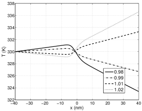
(a) Temperature

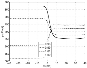
(b) Chemical potential

Figure 1: Temperature and chemical potential profiles at various $T^{\ell}$

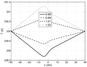
(a) Temperature

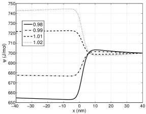
(b) Chemical potential

Figure 2: Temperature and chemical potential profiles at various $p^{g}$

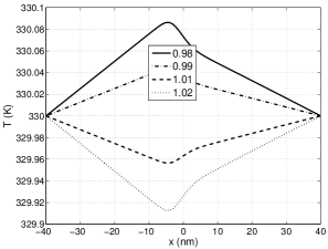
(a) Temperature

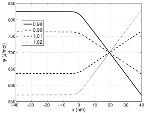
(b) Chemical potential

Figure 3: Temperature and chemical potential profiles at various $\zeta^{\ell}$

V Local equilibrium of the surface

In equilibrium it is possible to describe the surface in terms of Gibbs excess quantities Gibbs/ScientificPapers . One can treat a system of coexisting liquid and vapor as a three-phase system: liquid and vapor bulk phases and the surface phase. The surface has thermodynamic properties. The temperature and chemical potentials have the same equilibrium value as in the rest of the system. Furthermore the thermodynamic state of the surface is given by excess concentrations and thermodynamic potentials. Following Gibbs we have for the surface

$$\begin{array}[]{rl}h_{eq}^{s}&=\mu_{1,eq}\,c_{1,eq}^{s}+\mu_{2,eq}\,c_{2,eq}^{s}+T_{eq}\,s^{s}_{eq}\\ u_{eq}^{s}&=\mu_{1,eq}\,c_{1,eq}^{s}+\mu_{2,eq}\,c_{2,eq}^{s}+\gamma^{s}_{eq}+T_{eq}\,s^{s}_{eq}\\ f_{eq}^{s}&=\mu_{1,eq}\,c_{1,eq}^{s}+\mu_{2,eq}\,c_{2,eq}^{s}+\gamma^{s}_{eq}\\ g_{eq}^{s}&=\mu_{1,eq}\,c_{1,eq}^{s}+\mu_{2,eq}\,c_{2,eq}^{s}\\ \end{array}$$ (V.1)

The superscript $s$ indicates here the surface and equal to the excess of corresponding quantities. In these relations the temperature and the chemical potentials, which are the same everywhere, are independent of the choice of the dividing surface. The excesses depend on the choice of the dividing surface, in a such way that the above relations are true for any choice of the dividing surface.

It is our aim in this paper to show that the surface in a non-equilibrium liquid-vapor system can also be described as a separate thermodynamic phase using the Gibbs excess quantities. We will call this property the local equilibrium of the surface. The property of local equilibrium for the surface implies that it is possible to define all thermodynamic properties of a surface such that they have their equilibrium coexistence values for any choice of the dividing surface given the temperature of the surface $T^{s}$ and the chemical potential difference $\psi^{s}$. For this purpose we will define the excess densities and develop a method to obtain $T^{s}$ and $\psi^{s}$ independent of the choice of the dividing surface below. The analysis will be done using the numerical solution of the system in stationary non-equilibrium states.

V.1 Defining the excess densities.

The definition of the excesses consists of 3 steps: determining the phase boundaries, defining the specified dividing surface and, in particular, defining the excesses.

To determine the phase boundaries we will use the order parameter $q$. We introduce a small parameter $\beta$ and define the $\beta$-dependent boundary, $x^{g,s}_{\beta}$ between the vapor and the surface by

$$\left|\frac{q(x^{g,s}_{\beta})-q_{eos}(p_{\perp}(x^{g,s}_{\beta}),\,\xi(x^{g,s}_{\beta}),\,T(x^{g,s}_{\beta}))}{q(x^{g,s}_{\beta})}\right|\equiv\beta$$ (V.2)

where $q_{eos}(p_{\perp},\,\xi,\,T)$ is the equation of state’s value (no gradient contributions) of $q$ for pressure $p_{\perp}$, mass fraction $\xi$ and temperature $T$. The $\beta$-dependent boundary, $x^{\ell,s}_{\beta}$, between the surface and the liquid is defined in the same way.

The numerical procedure calculates profiles only at specified grid points, which we provide to the procedure. That means that $x^{g,s}_{\beta}$ and $x^{\ell,s}_{\beta}$ can only be situated at points of the grid. We choose their position to be the last bulk point of the grid where the left hand side of Eq. (V.2) does not exceed the right hand side. In our calculations we will choose $\beta=10^{-3}$ and use a grid of 81 points.

We shall also choose bulk boundaries near the box boundary where, because of the finite size of the box, the behavior of the profiles might be uncharacteristic. To avoid this effect, we do not consider the first 5 points of each phase close to these boundaries when we calculate the properties in these phases. The 6th point we call $x^{g}$ and the 76th point $x^{\ell}$.

The bulk gas therefore ranges from $x^{g}$ to $x^{g,s}_{\beta}$ and the bulk liquid ranges from $x^{\ell,s}_{\beta}$ to $x^{\ell}$. The surface therefore ranges from $x^{g,s}_{\beta}$ to $x^{\ell,s}_{\beta}$. In order to define excess quantities properly we always choose conditions such, that the bulk widths, $x^{g,s}_{\beta}-x^{g}$ and $x^{\ell}-x^{\ell,s}_{\beta}$ are larger then the surface width $x^{\ell,s}_{\beta}-x^{g,s}_{\beta}$.

In order to determine excess densities we need to extrapolate bulk profiles into the interfacial region. In equilibrium extrapolated bulk profiles are constants which are equal to the coexisting values of the corresponding quantities. Non-equilibrium bulk profiles are not constant. We fit the bulk profile with a polynomial of order $n_{b}=2$ and use this polynomial to extrapolate non-equilibrium bulk profiles into the interfacial region. This is done with the help of Matlab functions polyfit and polyval. It is important to realize that the extrapolation of the bulk profiles introduces a certain error depending on the choice of $\beta$ and $n_{b}$ in particular for non-equilibrium systems.

The distances between commonly used dividing surfaces, such as for instance the equimolar surface and the surface of tension, are very small. Thus, if there occurs an error in the determination of a dividing surface using a course grid, that would lead to inaccurate results. We therefore divide each interval of the course grid between $x^{g,s}_{\beta}$ and $x^{\ell,s}_{\beta}$ in $10^{4}$ subintervals. This surface grid is used for all operations related to the surface. Within the interfacial region we interpolate all the profiles (which were obtained by extrapolation from the bulk to the surface region using the course grid) from the course grid to the surface grid using a polynomial of order $n_{s}=3$ with the help of Matlab functions polyfit and polyval.

We can now define the excess $\widehat{\phi}$ of any density $\phi(x)$ as a function of a dividing surface $x^{\scriptstyle s}$ as

$$\widehat{\phi}(x^{\scriptstyle s})=\int_{\displaystyle x^{g,s}_{\beta}}^{\displaystyle x^{\ell,s}_{\beta}}{dx\,[\phi(x)-\phi^{g}(x)\,\Theta(x^{\scriptstyle s}-x)-\phi^{\ell}(x)\,\Theta(x-x^{\scriptstyle s})]}$$ (V.3)

where $\phi^{g}$ and $\phi^{\ell}$ are the extrapolated gas and liquid profiles and $\Theta(t)$ is the Heaviside function. The density $\phi$ is per unit of volume and $\widehat{\phi}$ is per unit of surface area. In our calculations integration is performed using the trapezoidal method by Matlab function trapz.

We can now define different dividing surfaces. The equimolar dividing surface $x^{c}$ is defined by the equation $\widehat{c}(x^{c})=0$. Analogously we define equimolar surfaces with respect to component 1 and 2: $\widehat{c}_{1}(x^{c_{1}})=0$ and $\widehat{c}_{2}(x^{c_{2}})=0$, and the equidensity surface $x^{\rho}$. The surface of tension $x^{\gamma}$ is defined from the equation $x^{\gamma}\,\widehat{p}_{\parallel}(x^{\gamma})-\widehat{x\,p_{\parallel}}(x^{\gamma})=0$. All the densities are given as arrays on a coordinate grid, but not as continuous functions. Thus, in order to find the solution of an equation $\varphi(x)=0$ we calculate the values $\varphi_{i}=\varphi(x_{i})$ for each point $x_{i}$ within the surface region and find the minimum of it’s absolute value, $\min_{i}(|\phi_{i}|)$. Because of the discrete nature of the argument this value may not be equal to zero, but it will be the closest to zero among all other coordinate points. So we will call this point the root of the equation $\varphi(x)=0$. We use the fine surface grid in this procedure.

If follows from Eq. (V.3) that

$$\frac{d\,\widehat{\phi}(x_{s})}{d\,x_{s}}=\phi^{\ell}(x_{s})-\phi^{g}(x_{s})$$ (V.4)

which we will use later.

V.2 Defining the temperature and chemical potential difference

An equilibrium two-phase two-component mixture has two free parameters, for instance the temperature $T$ and the chemical potential difference $\psi=\mu_{1}-\mu_{2}$. Local equilibrium of a surface implies, that in non-equilibrium it should be possible to define the temperature $T^{s}$ and the chemical potential difference $\psi^{s}$ of the surface. As found in ref. bedeaux/vdW/II for the surface temperature in the one-component system, both $T^{s}$ and $\psi^{s}$ should be independent of the choice of the dividing surface.

The equilibrium temperature and chemical potential difference determine all other equilibrium properties of the surface. Thus, there is a bijection from $T_{eq}$ and $\psi_{eq}$ to any other set of independent excess variables $X_{1,eq}$ and $X_{2,eq}$, so that one can use them equally well in order to characterize a surface. In non-equilibrium the temperature and chemical potential difference vary through the interfacial region, but as $X_{1,ne}$ and $X_{2,ne}$ are excesses, they characterize the whole surface. If a non-equilibrium surface is in local equilibrium, there should exist the same bijection. This implies that given two independent non-equilibrium excesses $X_{1,ne}$ and $X_{2,ne}$ one can determine the temperature $T^{s}$ and the chemical potential $\psi^{s}$ of the whole surface. Thus one can calculate equilibrium tables of $X_{1,eq}$($T_{eq}$, $\psi_{eq}$) and $X_{2,eq}$($T_{eq}$, $\psi_{eq}$) for different values of $T_{eq}$ and $\psi_{eq}$ and then determine temperature and chemical potential of a surface as $T^{s}=T_{eq}$($X_{1,ne}$, $X_{2,ne}$) and $\psi^{s}=\psi_{eq}$($X_{1,ne}$, $X_{2,ne}$).

As we want the temperature and chemical potential difference to be independent of the position of the dividing surface, we shall use excesses which are also independent of the position of a dividing surface in equilibrium for $X_{1}$ and $X_{2}$. For two component mixture these independent variables are the surface tension $\gamma$ and the relative adsorption $\Gamma_{12}$. If the number of components is more then 2, additional relative adsorptions should be used.

These quantities are well defined for equilibrium, but not for non-equilibrium. So we will define them first. In equilibrium the surface tension is defined as minus the excess of the parallel pressure $\gamma_{eq}=-\widehat{p}_{\parallel}$. Alternatively one often uses the integral of $p_{\perp}-p_{\parallel}(x)\equiv\gamma_{xx}(x)$ across the interface: $\gamma_{eq}=\int{dx\,\gamma_{xx}(x)}$. Both definitions are equivalent in equilibrium since $p_{\perp}$ is constant through the interface and $\gamma_{xx}(x)$ is identically zero in the bulk phases. In non-equilibrium $\gamma_{xx}(x)$ may differ from zero in the bulk regions, however, and this makes the second definition inappropriate. We will therefore define the non-equilibrium surface tension using the standard definition

$$\gamma(x^{\scriptstyle s})=-\widehat{p}_{\parallel}(x^{\scriptstyle s})$$ (V.5)

This quantity differs from $\widehat{\gamma}_{xx}$ by the term equal to $\widehat{p}_{\perp}$, which is usually small compared to $\widehat{p}_{\parallel}$.

The relative adsorption is defined as $\Gamma_{12,eq}=\widehat{c}_{1,eq}-\widehat{c}_{2,eq}\,(c^{\ell}_{1,eq}-c^{g}_{1,eq})/(c^{\ell}_{2,eq}-c^{g}_{2,eq})$ in equilibrium DefayPrigogine/sta , where $c^{\ell}_{i,eq}$ and $c^{g}_{i,eq}$ are coexistence concentrations of the corresponding components. Since these quantities are not constant in non-equilibrium, we cannot use this definition directly. One can however see from Eq. (V.4), that both, in equilibrium and non-equilibrium $\widehat{c}_{i}\,^{\prime}(x^{\scriptstyle s})=c^{\ell}_{i}(x^{\scriptstyle s})-c^{g}_{i}(x^{\scriptstyle s})$, where the prime indicates a spatial derivative. Since in equilibrium $c^{\ell}_{i}(x^{\scriptstyle s})-c^{g}_{i}(x^{\scriptstyle s})=c^{\ell}_{i,eq}-c^{g}_{i,eq}$ we can use the following definition

$$\Gamma_{12}(x^{\scriptstyle s})=\widehat{c}_{1}(x^{\scriptstyle s})-\widehat{c}_{2}(x^{\scriptstyle s})\,{\frac{c^{\ell}_{1}(x^{\scriptstyle s})-c^{g}_{1}(x^{\scriptstyle s})}{c^{\ell}_{2}(x^{\scriptstyle s})-c^{g}_{2}(x^{\scriptstyle s})}}$$ (V.6)

both in equilibrium and non-equilibrium.

If the system is in local equilibrium we may write:

$$\begin{array}[]{rl}\gamma(x^{\scriptstyle s})&=\gamma_{eq}(T^{s},\psi^{s})\\ \Gamma_{12}(x^{\scriptstyle s})&=\widehat{c}_{1}(x^{\scriptstyle s})-\widehat{c}_{2}(x^{\scriptstyle s})\,\displaystyle{\frac{c^{\ell}_{1,eq}(T^{s},\psi^{s})-c^{g}_{1,eq}(T^{s},\psi^{s})}{c^{\ell}_{2,eq}(T^{s},\psi^{s})-c^{g}_{2,eq}(T^{s},\psi^{s})}}\end{array}$$ (V.7)

Substituting the expressions for $\gamma(x_{s})$ and $\Gamma_{12}(x_{s})$ from Eq. (V.5) and Eq. (V.6) into Eq. (V.7) we obtain the following relations

$$\begin{array}[]{rl}\widehat{p}_{\parallel}(x^{\scriptstyle s})&=\widehat{p}_{\parallel,eq}(T^{s},\psi^{s})\\ \\ \displaystyle{\frac{c^{\ell}_{1}(x^{\scriptstyle s})-c^{g}_{1}(x^{\scriptstyle s})}{c^{\ell}_{2}(x^{\scriptstyle s})-c^{g}_{2}(x^{\scriptstyle s})}}&=\displaystyle{\frac{c^{\ell}_{1,eq}(T^{s},\psi^{s})-c^{g}_{1,eq}(T^{s},\psi^{s})}{c^{\ell}_{2,eq}(T^{s},\psi^{s})-c^{g}_{2,eq}(T^{s},\psi^{s})}}\end{array}$$ (V.8)

This gives the bijection equations to determine $T^{s}$ and $\psi^{s}$ from the actual non-equilibrium variables. As the left hand sides in Eq. (V.8) are in good approximation independent of the position of the dividing surface, $T^{s}$ and $\psi^{s}$ are similarly independent on this position.

V.3 Defining local equilibrium

The other quantities required for the Gibbs description of the non-equilibrium surfaces we define in the following way. The surface chemical potentials are the equilibrium coexistence values determined via the procedure discussed in Subsec. [III.1]

$$\begin{array}[]{rl}\mu_{1}^{s}&\equiv\mu_{1,\,eq}(T^{s},\psi^{s})\\ \mu_{2}^{s}&\equiv\mu_{2,\,eq}(T^{s},\psi^{s})\\ \end{array}$$ (V.9)

We define the surface extensive properties as

$$\phi^{s}(x^{\scriptstyle s})\equiv\widehat{\phi}(x^{\scriptstyle s})$$ (V.10)

The local equilibrium of a surface should be established for any choice of a dividing surface. The results of the calculations for any particular choice of a dividing surface may not be representative since they may be different differ for another choice of a dividing surface. Thus, the property of local equilibrium should be established for all dividing surfaces together.

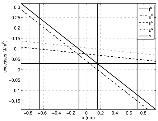
Figure 4: Equilibrium excesses at $T=330$ K and $\psi=700$ J/mol. The vertical lines indicate the $x^{c_{2}}$, $x^{\gamma}$, $x^{c}$, $x^{c_{1}}$ dividing surfaces from left to right.

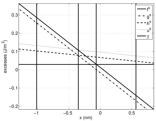
Figure 5: Non-equilibrium excesses for the case of perturbing $T^{\ell}=1.02\,T_{eq}$. The vertical lines indicate the $x^{c_{2}}$, $x^{\gamma}$, $x^{c}$, $x^{c_{1}}$ dividing surfaces from left to right.

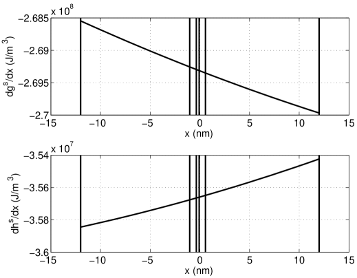
Figure 6: Slopes of non-equilibrium excesses for the case of perturbing $T^{\ell}=1.02\,T_{eq}$. The vertical lines indicate the surface boundaries and $x^{c_{2}}$, $x^{\gamma}$, $x^{c}$, $x^{c_{1}}$ dividing surfaces.

Consider the profile of an excess $\widehat{\phi}(x^{\scriptstyle s})$ as a function of position of a dividing surface $x^{\scriptstyle s}$. It follows from Eq. (V.4) that the slope of the excess profile is equal to the difference between the extrapolated values of a profile of thermodynamic quantity $\phi$. In equilibrium these values are constant and equal to the coexistence values. Thus, equilibrium excess profiles are straight lines, as one can see on Fig. [4]. Non-equilibrium profiles in the bulk phases are not constant. We construct the extrapolated profiles using $n_{b}$th order polynomials with $n_{b}=2$. Resulting non-equilibrium excesses are therefore polynomials of the order $n_{b}+1=3$, according to Eq. (V.4). These profiles, for the most extreme case of non-equilibrium perturbation $T^{\ell}=1.02\,T_{eq}$, are shown in Fig. [5]. Even though these profiles are polynomials of the 3rd order they are very close to straight lines. As one can see from Fig. [6] the variation in the slope is about 1% through the whole surface. It indicates that this non-equilibrium ”state” is very close to an equilibrium one.

We therefore develop the procedure to relate the non-equilibrium state to an equilibrium one by comparing thermodynamic quantities in equilibrium and in non-equilibrium. The comparison performed in one particular point of the surface may not be sufficient because it may suffer from artefacts peculiar to this particular surface. Moreover, any comparison performed in a particular point does not speak for the whole. We therefore compare the non-equilibrium surface with an equilibrium one for all dividing surfaces together. We will use the least square sum method for this.

Consider a non-equilibrium thermodynamic excess $t^{s}(x^{\scriptstyle s})$ and a quantity $r^{s}(x^{\scriptstyle s};T,\psi)$ which is a combination of excesses and may depend on $(T,\psi)$ as parameters. We introduce the following measures of the difference of $t^{s}$ and $r^{s}$

$$\delta_{t^{\scriptstyle s},r^{\scriptstyle s}}(x^{\scriptstyle s};T,\psi)\equiv|t^{s}(x^{\scriptstyle s}_{i})-r^{s}(x^{\scriptstyle s}_{i};T,\psi)|$$ (V.11)

and

$$\begin{array}[]{rl}S_{t^{\scriptstyle s},r^{\scriptstyle s}}(T,\psi)&\equiv\displaystyle\sum_{i\,\in\,surface}{\left[t^{s}(x^{\scriptstyle s}_{i})-r^{s}(x^{\scriptstyle s}_{i};T,\psi)\right]^{2}}\\ \\ \sigma_{t^{\scriptstyle s},r^{\scriptstyle s}}(T,\psi)&\equiv\displaystyle{1\over N}\,\sqrt{S_{t^{\scriptstyle s},r^{\scriptstyle s}}(T,\psi)}\end{array}$$ (V.12)

where $N$ is the number of surface points.

We say that $t^{s}$ and $r^{s}$ are the same in the surface if the value of $\sigma_{t^{\scriptstyle s},r^{\scriptstyle s}}(T,\psi)$ is negligible compared to the typical value of either $|t^{s}(x^{\scriptstyle s})|$ or $|r^{s}(x^{\scriptstyle s};T,\psi)|$. If two quantities $t^{s}$ and $r^{s}$ are the same in the above sense, we say that the non-equilibrium state of the surface is characterized by surface temperature $T^{s}_{{\scriptstyle\{x^{\scriptstyle s}\}}}$ and chemical potential difference $\psi^{s}_{{\scriptstyle\{x^{\scriptstyle s}\}}}$ if

$$S_{t^{\scriptstyle s},r^{\scriptstyle s}}(T^{s}_{{\scriptstyle\{x^{\scriptstyle s}\}}},\psi^{s}_{{\scriptstyle\{x^{\scriptstyle s}\}}})=\min_{T,\psi}S_{t^{\scriptstyle s},r^{\scriptstyle s}}(T,\psi)$$ (V.13)

Here superscript $s$ indicates that we speak about surface quantities only (as everywhere in this paper) and subscript ${\scriptstyle\{x^{\scriptstyle s}\}}$ indicates that $T^{s}_{{\scriptstyle\{x^{\scriptstyle s}\}}}$ and $\psi^{s}_{{\scriptstyle\{x^{\scriptstyle s}\}}}$ are the parameters for all dividing surfaces together (in contrast to the values $T^{s}(x^{\scriptstyle s})$ and $\psi^{s}(x^{\scriptstyle s})$ determined from Eq. (V.8) for each particular dividing surface $x^{\scriptstyle s}$).

These definitions are easy to illustrate in equilibrium. For instance, for $h^{s}_{eq,\,gibbs}(x^{\scriptstyle s};T,\psi)\equiv\mu_{1,eq}(T,\psi)\,c_{1,eq}^{s}+\mu_{2,eq}(T,\psi)\,c_{2,eq}^{s}+T\,s^{s}_{eq}$ it follows from Eq. (V.1), that $h^{s}_{eq}(x^{\scriptstyle s};T_{eq},\psi_{eq})=h^{s}_{eq,\,gibbs}(x^{\scriptstyle s};T_{eq},\psi_{eq})$. Furthermore $g^{s}_{eq}(x^{\scriptstyle s};T_{eq},\psi_{eq})\neq h^{s}_{eq,\,gibbs}(x^{\scriptstyle s};T_{eq},\psi_{eq})$. Thus $\delta_{h^{\scriptstyle s}_{\vphantom{\scriptstyle gibbs}\scriptstyle eq},\,h^{\scriptstyle s}_{\scriptstyle eq,\,gibbs}}(x^{\scriptstyle s};T_{eq},\psi_{eq})=0$ and $\delta_{g^{\scriptstyle s}_{\vphantom{\scriptstyle gibbs}\scriptstyle eq},\,h^{\scriptstyle s}_{\scriptstyle eq,\,gibbs}}(x^{\scriptstyle s};T_{eq},\psi_{eq})\neq 0$. It is also true that $S_{h^{\scriptstyle s}_{\vphantom{\scriptstyle gibbs}\scriptstyle eq},\,h^{\scriptstyle s}_{\scriptstyle eq,\,gibbs}}(T_{eq},\psi_{eq})=\min S_{h^{\scriptstyle s}_{\vphantom{\scriptstyle gibbs}\scriptstyle eq},\,h^{\scriptstyle s}_{\scriptstyle eq,\,gibbs}}(T,\psi)$ and $\sigma_{h^{\scriptstyle s}_{\vphantom{\scriptstyle gibbs}\scriptstyle eq},\,h^{\scriptstyle s}_{\scriptstyle eq,\,gibbs}}(T,\psi)\ll\sigma_{g^{\scriptstyle s}_{\vphantom{\scriptstyle gibbs}\scriptstyle eq},\,h^{\scriptstyle s}_{\scriptstyle eq,\,gibbs}}(T,\psi)$. According to the above definitions i) $h^{s}_{eq,\,gibbs}$ and $h^{s}_{eq}$ are the same quantities, but $h^{s}_{eq,\,gibbs}$ and $g^{s}_{eq}$ are not the same; ii) the equilibrium state is characterized by $(T_{eq},\psi_{eq})$; as it should be. While this analysis is trivial in equilibrium, it is not trivial in non-equilibrium.

Note, that while in equilibrium the conditions $\delta_{t,r}(x^{\scriptstyle s};T_{eq},\psi_{eq})=0$ and $S_{t,r}(T_{eq},\psi_{eq})=\min S_{t,t}(T,\psi)$ are equivalent, in general it does not follow in non-equilibrium from Eq. (V.13) that

$$\delta_{t,r}(x^{\scriptstyle s};T,\psi)=0\quad\forall\;x^{\scriptstyle s}$$ (V.14)

Thus Eq. (V.14) is not a good measure of the equality of the quantities and states in non-equilibrium. We may therefore speak about the equality of thermodynamic quantities as well as about the state $T^{s}$ and $\psi^{s}$ of the surface in non-equilibrium only in the least square sense, as it is given in Eq. (V.13).

Within establishing the local equilibrium property of a non-equilibrium surface we would like to verify the following properties: i) the existence of the unique temperature $T^{s}$ and chemical potential difference $\psi^{s}$ of a non-equilibrium surface; ii) the validity of the Eq. (V.1) in non-equilibrium at the surface’s $T^{s}$ and $\psi^{s}$; iii) the possibility to determine all the properties of a non-equilibrium surface from equilibrium tables at the surface’s $T^{s}$ and $\psi^{s}$. We do this in the following section.

VI Verification of local equilibrium.

We calculate the the equilibrium properties (coexistence data, such as the pressure or bulk densities, as well as various excesses) of the system for the range of temperatures $T=\{325,326,\ldots,340\}$ K and the range of chemical potentials $\psi=\{400,450,\ldots,1000\}$ J/mol. The value of a thermodynamic quantity at any point $(T,\psi)$, which is between these is interpolated using the Matlab procedures interp2 and griddata.

VI.1 Surface temperature and chemical potential difference

As was mentioned, in equilibrium both $\gamma$ and $\Gamma_{12}$ are independent of the location of the dividing surface $x^{\scriptstyle s}$. Given the above definitions, Eq. (V.5) and Eq. (V.6), we can calculate these quantities for non-equilibrium states. Calculations show, that even though $\gamma$ and $\Gamma_{12}$ are not exactly independent on $x^{\scriptstyle s}$ away from equilibrium, the relative deviation is so small (about $0.004\%$ for $\gamma$ and $4\%$ for $\Gamma_{12}$ in the worst case), that one can consider these quantities to be independent of the position of the dividing surface. Thus one may use them in order to find the temperature, $T^{s}$, and the chemical potential difference, $\psi^{s}$, of the surface in non-equilibrium states, which will be independent of the position of the dividing surface.

Using Eq. (V.12) and Eq. (V.8) together with Eq. (V.4) we construct the following expressions

$$\begin{array}[]{rl}S_{\gamma}(T,\psi)&=\displaystyle\sum_{x^{\scriptstyle s}}{\left[\widehat{p}_{\parallel}(x^{\scriptstyle s})-\widehat{p}_{\parallel,eq}(T,\psi)\right]^{2}}\\ \\ S_{\Gamma_{12}}(T,\psi)&=\displaystyle\sum_{x^{\scriptstyle s}}{\left[{\frac{\widehat{c}^{\;\prime}_{1,eq}(x^{\scriptstyle s};T,\psi)}{\widehat{c}^{\;\prime}_{1}(x^{\scriptstyle s})}}-{\frac{\widehat{c}^{\;\prime}_{2,eq}(x^{\scriptstyle s};T,\psi)}{\widehat{c}^{\;\prime}_{2}(x^{\scriptstyle s})}}\right]^{2}}\\ \end{array}$$ (VI.1)

where the prime indicates the derivative with respect to $x^{\scriptstyle s}$.

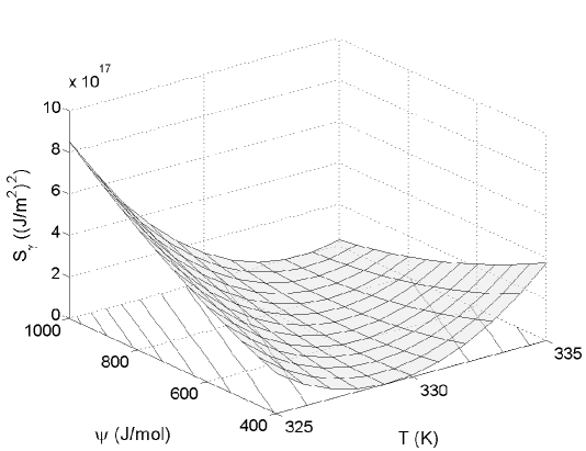
Figure 7: The plot of $S_{t}(T,\psi)$ for $t$ being the profile of the surface tension $\gamma$ for the case of perturbing $T^{\ell}=1.02\,T_{eq}$. The lines in the $T$-$\psi$ plane are lines of constant value of $S_{t}(T,\psi)$

$S_{i}(T,\psi)$ (where $i$ is either $\gamma$ or $\Gamma_{12}$) should reach the minimum at $T^{s}_{{\scriptstyle\{x^{\scriptstyle s}\}}}$ and $\psi^{s}_{{\scriptstyle\{x^{\scriptstyle s}\}}}$. We note however, that neither $S_{i}(T,\psi)$ have a minimum at a single point $(T^{s},\psi^{s})$. There is a whole generatrix curve of minima $C_{i}(T,\psi)=0$ so the plot of $S_{i}(T,\psi)$ is a valley. One can see it on Fig. [7]. Every point of the generatrix curve is the minimum point of $S_{i}(T,\psi)$ along the direction ”perpendicular” to this generatrix. If $\widehat{p}_{\parallel}(x^{\scriptstyle s})$ or $\widehat{c}^{\;\prime}_{1}(x^{\scriptstyle s})$ and $\widehat{c}^{\;\prime}_{2}(x^{\scriptstyle s})$ represent the corresponding profiles for some equilibrium state $(T_{eq},\psi_{eq})$, then $S_{i}(T,\psi)=0$ and the generatrix is constant. Since these profiles are non-equilibrium profiles, the generatrix is not exactly constant but very close to it. Thus $C_{i}(T,\psi)={\partial S_{i}(T,\psi)}/{\partial w}$, where $w$ is a direction in $T$-$\psi$ plane which is perpendicular to generatrix. In fact, one should be careful speaking about directions, since no metric is defined in the $T$-$\psi$ plane. Thus we cannot introduce $\nabla_{T\psi}$ so that $C_{i}(T,\psi)=|\nabla_{T\psi}S_{i}(T,\psi)|$. In fact, $w$ can be any direction which does not coincide or does not almost coincide with the direction of generatrix. In practice we find that we can use $w=T$, while using $w=\psi$ gives less accurate results. Thus we determine the minima curve from the equation

$$\frac{\partial S_{i}(T,\psi)}{\partial T}=0$$ (VI.2)

Thus one needs two quantities $S_{\gamma}$ and $S_{\Gamma}$ in order to determine $T^{s}_{{\scriptstyle\{x^{\scriptstyle s}\}}}$ and $\psi^{s}_{{\scriptstyle\{x^{\scriptstyle s}\}}}$ uniquely. The surface temperature and chemical potential difference $T^{s}_{{\scriptstyle\{x^{\scriptstyle s}\}}}$ and $\psi^{s}_{{\scriptstyle\{x^{\scriptstyle s}\}}}$ are determined from the intersection of two minimum curves of $S_{\gamma}$ and $S_{\Gamma}$

$$\begin{array}[]{rl}\displaystyle\left.\frac{\partial S_{\gamma}(T,\psi)}{\partial T}\right|_{\,T^{\scriptstyle s}_{{\scriptstyle\{x^{\scriptstyle s}\}}},\,\psi^{s}_{{\scriptstyle\{x^{\scriptstyle s}\}}}}&=0\\ \displaystyle\left.\frac{\partial S_{\Gamma_{12}}(T,\psi)}{\partial T}\right|_{\,T^{\scriptstyle s}_{{\scriptstyle\{x^{\scriptstyle s}\}}},\,\psi^{s}_{{\scriptstyle\{x^{\scriptstyle s}\}}}}&=0\\ \end{array}$$ (VI.3)

We calculate the temperatures and the chemical potential differences for different non-equilibrium conditions. They are outlined in Tables [LABEL:tbl/TP/Tl-LABEL:tbl/TP/zil]. The first row of each table, corresponding to ${\scriptstyle\{x^{\scriptstyle s}\}}$, gives $T^{s}$ and $\psi^{s}$ calculated from Eq. (VI.3). The following rows give, corresponding to different particular dividing surfaces, gives $T^{s}$ and $\psi^{s}$ calculated from Eq. (V.8).

Table 3: Surface temperatures (K) and chemical potentials (J/mol) for the case of perturbing $T^{\ell}$

	$T^{\ell}=1.02\,T_{eq}$		$T^{\ell}=0.98\,T_{eq}$
surface	$T^{s}$	$\psi^{s}$	$T^{s}$	$\psi^{s}$
${\scriptstyle\{x^{\scriptstyle s}\}}$	331.831	770.53	328.129	650.92
$x^{c}$	331.823	769.51	328.124	650.29
$x^{\gamma}$	331.828	770.22	328.123	650.21
$x^{c_{1}}$	331.814	767.97	328.127	650.43
$x^{c_{2}}$	331.838	771.86	328.121	650.1

Table 4: Surface temperatures (K) and chemical potentials (J/mol) for the case of perturbing $p^{g}$

	$p^{g}=1.02\,p_{eq}$		$p^{g}=0.98\,p_{eq}$
surface	$T^{s}$	$\psi^{s}$	$T^{s}$	$\psi^{s}$
${\scriptstyle\{x^{\scriptstyle s}\}}$	330.796	683.87	329.059	696.52
$x^{c}$	330.8	684.68	329.063	697.22
$x^{\gamma}$	330.799	684.44	329.063	697.12
$x^{c_{1}}$	330.804	685.19	329.065	697.46
$x^{c_{2}}$	330.795	683.93	329.061	696.87

Table 5: Surface temperatures (K) and chemical potentials (J/mol) for the case of perturbing $\zeta^{\ell}$

	$\zeta^{\ell}=1.02\,\zeta^{\ell}_{eq}$		$\zeta^{\ell}=0.98\,\zeta^{\ell}_{eq}$
surface	$T^{s}$	$\psi^{s}$	$T^{s}$	$\psi^{s}$
${\scriptstyle\{x^{\scriptstyle s}\}}$	329.577	559.32	330.24	812.86
$x^{c}$	329.598	562.44	330.242	813.16
$x^{\gamma}$	329.584	560.5	330.253	814.67
$x^{c_{1}}$	329.63	566.83	330.219	809.99
$x^{c_{2}}$	329.554	556.3	330.278	817.99

Note, that $T^{s}$ and $\psi^{s}$ may be different from the continuous values in the interfacial region.

VI.2 The non-equilibrium Gibbs surface

In this section we would like to verify that the surface quantities defined by Eq. (V.10) satisfy Eq. (VI.4) with $T^{s}$ and $\psi^{s}$ determined by Eq. (V.8) and Eq. (VI.3).

$$\phi^{s}=\phi_{gibbs}^{s}(T^{s},\psi^{s})$$ (VI.4)

namely, with the definition Eq. (V.9),

$$\begin{array}[]{rl}h^{s}&=\mu_{1}^{s}\,c_{1}^{s}+\mu_{2}^{s}\,c_{2}^{s}+T^{s}\,s^{s}\\ u^{s}&=\mu_{1}^{s}\,c_{1}^{s}+\mu_{2}^{s}\,c_{2}^{s}+\gamma^{s}+T^{s}\,s^{s}\\ f^{s}&=\mu_{1}^{s}\,c_{1}^{s}+\mu_{2}^{s}\,c_{2}^{s}+\gamma^{s}\\ g^{s}&=\mu_{1}^{s}\,c_{1}^{s}+\mu_{2}^{s}\,c_{2}^{s}\\ \end{array}$$ (VI.5)

where the right hand side is $\phi_{gibbs}^{s}(T^{s},\psi^{s})$ of the corresponding quantity. Eq. (VI.5) is the non-equilibrium analogon of equilibrium Eq. (V.1).

In order to analyze the measure of validity of Eq. (VI.4) we construct the quantity

$$\begin{array}[]{rl}\displaystyle\mathcal{E}_{\phi_{gibbs}}(T,\psi)&=\displaystyle\sum_{i\,\in\,surface}{\left[\frac{\phi^{s}(x^{\scriptstyle s}_{i})-\phi^{s}_{gibbs}(x^{\scriptstyle s}_{i};\,T,\psi)}{\phi^{s}(x^{\scriptstyle s}_{i})}\right]^{2}}\\ \\ \displaystyle\epsilon_{\phi_{gibbs}}(x^{\scriptstyle s};T,\psi)&=\displaystyle\left|\frac{\phi^{s}(x^{\scriptstyle s})-\phi^{s}_{gibbs}(x^{\scriptstyle s};T,\psi)}{\phi^{s}(x^{\scriptstyle s})}\right|\end{array}$$ (VI.6)

for each thermodynamic potential $h$, $u$, $f$, $g$. $\mathcal{E}_{\phi_{gibbs}}$ gives the relative error of the determination of the surface quantity $\phi^{s}$ using the Gibbs excesses relations Eq. (VI.5) for for all dividing surfaces together, while $\epsilon_{\phi_{gibbs}}$ gives this error for particular dividing surface. We build $\mathcal{E}_{\phi_{gibbs}}(T,\psi)$ for $T=T^{s}_{{\scriptstyle\{x^{\scriptstyle s}\}}}$, $\psi=\psi^{s}_{{\scriptstyle\{x^{\scriptstyle s}\}}}$ determined from Eq. (VI.3) only for the whole surface. We build $\epsilon_{\phi_{gibbs}}(T,\psi)$ both for $T=T^{s}_{{\scriptstyle\{x^{\scriptstyle s}\}}}$, $\psi=\psi^{s}_{{\scriptstyle\{x^{\scriptstyle s}\}}}$ determined for the whole surface and for $T=T^{s}(x^{\scriptstyle s})$, $\psi=\psi^{s}(x^{\scriptstyle s})$ determined from Eq. (V.8) for particular dividing surface. The values of the corresponding errors are listed in Tables [LABEL:tbl/Gibbs/Tl-LABEL:tbl/Gibbs/zil] in Subsec. [A.1], and are found to be small.

As one can see, there is a variation in the value of the error for the different dividing surfaces. It is caused by two reasons. The first reason for this is slight variation in $T^{s}$ and $\psi^{s}$ from Tables [LABEL:tbl/TP/Tl-LABEL:tbl/TP/zil] for different dividing surfaces. The variation of each excess potential corresponds to the variation of $T^{s}$ and $\psi^{s}$ through these surfaces. Thus so do the relative errors.

Another factor which influences the value of these errors is the actual value of an excess at a given dividing surface. If it is close to zero, then in the expression for $\epsilon$ the small value is in denominator and it gives the huge value for the error. Particularly, $g^{s}(x^{c})\approx 0$ both in equilibrium and in non-equilibrium which makes the row corresponding to $g$ at $x^{c}$ be uninformative and one should not take into account these data.

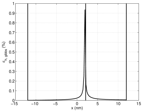
Figure 8: The relative error $\epsilon_{h_{gibbs}}(x^{\scriptstyle s};T^{s}_{{\scriptstyle\{x^{\scriptstyle s}\}}},\psi^{s}_{{\scriptstyle\{x^{\scriptstyle s}\}}})$ for the case of perturbing $T^{\ell}=1.02\,T_{eq}$. The vertical lines indicate the surface boundaries and $x^{h}$ dividing surfaces.

We emphasize however that the overall error $\mathcal{E}_{\phi_{gibbs}}$ represents the whole surface and thus do not suffer from the fact that some quantity is negligible at some dividing surface. There are such points for each potential $\phi$, however their contribution to the whole error is negligible itself. So we can see, that if the particular dividing surface is far from zero point of $\phi$, $\epsilon_{\phi_{gibbs}}$ gives the good measure of the error. While if the particular dividing surface is close to zero point of $\phi$, $\epsilon_{\phi_{gibbs}}$ fails to measure the error. One can see from Fig. [8] that the relative error $\epsilon_{\phi_{gibbs}}$ indeed rises enormously at $x^{\phi}$. Particularly because of this fact the definition of the excess quantities in bedeaux/vdW/II was different from Eq. (V.10).

Another possible test is to compare the absolute error $|\phi^{s}(x^{\scriptstyle s})-\phi^{s}_{gibbs}(x^{\scriptstyle s};T,\psi^{s})|$ with the deviation $\sigma_{\phi_{gibbs}}(T,\psi)$ defined in Eq. (V.12). The calculations show that for the particular dividing surfaces the former quantity does not exceed the lateral, which indicates that all the absolute errors are actually within the trust region.

VI.3 Equilibrium tables

In this subsection we will verify the possibility to determine all the properties of a non-equilibrium surface from equilibrium tables at the surface’s $T^{s}$ and $\psi^{s}$. The surface chemical potentials $\mu_{1}^{s}$ and $\mu_{2}^{s}$ are already defined as their equilibrium values by Eq. (V.9). So in this section we will verify the relation

$$\phi^{s}=\phi^{s}_{eq}(T^{s},\psi^{s})$$ (VI.7)

As in Subsec. [VI.2] we compare the actual excess of a thermodynamic potential with the corresponding equilibrium value at given temperature and chemical potential of the surface. Before we do this a note has to be made.

Under non-equilibrium conditions the profile of a quantity $\phi^{s}$ is shifted with respect to the equilibrium one. One can see this in the example for $\phi=h$ in Fig. [9]. The reason for this are fluxes caused by non-equilibrium perturbation. The whole surface is therefore shifted. One can clearly see that comparing the positions of the particular dividing surfaces on Fig. [4] and Fig. [5]. So the direct comparison of the profiles should be done not in the observer’s frame of reference (OFO, which is used in all other calculations), but in the surface’s frame of reference (SFO). The SFO is simply shifted with respect to the OFO, depending on the rate of non-equilibrium perturbations. Zero of the SFO is chosen at the reference surface, which can be either the equimolar surface, or any other physically sensible surface. If $x^{\ominus}$ is the position of this surface in OFO and $\phi^{s}_{\mathrm{OFO}}(x^{s}_{\mathrm{OFO}})$ is the profile of $\phi^{s}$ in OFO, then $\phi^{s}_{\mathrm{SFO}}(x^{s}_{\mathrm{SFO}})\equiv\phi^{s}_{\mathrm{OFO}}(x^{s}_{\mathrm{OFO}})=\phi^{s}_{\mathrm{OFO}}(x^{s}_{\mathrm{SFO}}+x^{\ominus})$ is the profile of $\phi^{s}$ in SFO.

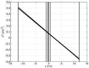
(a) Whole surface

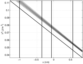
(b) Subregion

Figure 9: Non-equilibrium profile of $h^{s}$ for the case of perturbing $T^{\ell}=1.02\,T_{eq}$ (solid line) compared to the profiles of $h^{s}_{eq}$ calculated from the equilibrium tables for different $T_{eq}$ and $\psi_{eq}$ (dotted lines). The vertical lines indicate the surface boundaries and dividing surfaces for non-equilibrium case.

We can now determine to which equilibrium state the non-equilibrium one should correspond. Consider the following definitions of $\mathcal{E}_{\phi_{table}}$ and $\epsilon_{\phi_{table}}$ which have the same meaning as in Eq. (VI.6):

$$\begin{array}[]{rl}\displaystyle\mathcal{E}_{\phi_{table}}(T,\psi)&=\displaystyle\sum_{i\,\in\,surface}{\left[\frac{\phi^{s}(x^{\scriptstyle s}_{i})-\phi^{s}_{eq}(x^{\scriptstyle s}_{i}+x^{\ominus}_{eq}-x^{\ominus};\,T,\psi)}{\phi^{s}(x^{\scriptstyle s}_{i})}\right]^{2}}\\ \\ \displaystyle\epsilon_{\phi_{table}}(x^{\scriptstyle s};T,\psi)&=\displaystyle\left|\frac{\phi^{s}(x^{\scriptstyle s})-\phi^{s}_{eq}(x^{\scriptstyle s};T,\psi)}{\phi^{s}(x^{\scriptstyle s})}\right|\end{array}$$ (VI.8)

for each thermodynamic potential $h$, $u$, $f$, $g$. $x^{\ominus}$ and $x^{\ominus}_{eq}$ are the non-equilibrium and equilibrium positions of the reference surface in OFO. The set $\{x^{\scriptstyle s}_{i}\}$ is the non-equilibrium surface grid and is used for both profiles. Since the width of an equilibrium surface may be not the same as the non-equilibrium one, the summation may exceed the formal boundaries of the equilibrium surface. This is not a problem however, since the equilibrium profile $\psi^{s}_{eq}$ is the line with constant slope everywhere, as well as beyond the formal boundaries. We don’t shift the surface grid in the definition of $\epsilon_{\phi_{table}}(x^{\scriptstyle s};T,\psi)$ because in that notation $x^{\scriptstyle s}$ means the particular dividing surface, while $x^{\scriptstyle s}_{i}$ means the point of the surface grid.

The values of the corresponding errors are listed in Tables [LABEL:tbl/Table/Tl-LABEL:tbl/Table/zil] in Subsec. [A.2], and are found to be small.

As in Subsec. [VI.2] we see, that for the equimolar surface the relative error in $g$ is huge. There is the same reason for this, namely that $g^{s}(x_{c})\approx 0$ both in equilibrium and in non-equilibrium. This again makes the row corresponding to $g$ at $x^{c}$ be uninformative and one should not take into account these data.

VII Conclusions

The article continues the general analysis started in glav/grad1 . Here we focus on a specified mixture and develop further its properties. We choose a binary mixture of cyclohexane and $n$-hexane as the system and describe in details how to implement the general analysis presented in glav/grad1 . We build numerical procedure for solving the resulted system of differential equations. The resulted profiles of continuous variables are presented in Sec. [IV] and in the first article. We see, in particular, that a two component mixture develop the temperature profile in the surface region which is similar to the temperature profile obtained for one-component system bedeaux/vdW/I . Another characteristic of a binary mixture is the difference between chemical potentials of components. The behavior of the profile of $\psi$ in non-equilibrium steady-states is different. It has different values in the different bulk phases and we observe a transition from the one value to the other in the surface region.

We then proceed to verify the local equilibrium of the surface. This property means that a surface under non-equilibrium steady-state conditions can be described as equilibrium one in terms of the Gibbs excess densities. We have discussed the meaning of the surface quantities in non-equilibrium and established the systematic procedure to obtain them. We were in particular focused on i) the existence of the unique surface’s temperature and chemical potential difference; ii) the validity of the relations between thermodynamic Gibbs excesses in a non-equilibrium surface; iii) the correspondence between the non-equilibrium and equilibrium properties of the surface. It was possible to verify that one can speak about these statements independently on the choice of the dividing surface. Similar results for the one-component system were obtained in bedeaux/vdW/II .

The extrapolations procedure is numerical, and contains therefore a certain error. We may not expect this error to be negligible, not only because of numerical inaccuracy, but also because of the non-equilibrium nature of the system. If the error is within a reasonable range, we will consider this as a satisfactory verification of local equilibrium.

The main part of the analysis in the interfacial region is introducing the excesses of thermodynamic densities, which are constructed with the help of extrapolated bulk profiles. In contrast to equilibrium, non-equilibrium bulk profiles are not constants, and therefore their extrapolation to the surface region is not always accurate. The accuracy of extrapolation lowers when the surface width increases. Apparent small deviations from local equilibrium are therefore to some extent an artefact of the inaccuracy of the extrapolation.

In the description of the surface excess densities it may happen that for particular choice of the dividing surface not one but several of the excesses are negligible. This increases the relative error enormously while the absolute error remains finite and more or less constant. In order to avoid this problem we consider the excesses for all dividing surfaces together, rather then for a particular dividing surface. Particularly, in bedeaux/vdW/II the definition of the excess Gibbs energy was chosen differently because this excess was very small for the equimolar surface. We have shown in this paper why this is not needed.

One can see from these data, that within different ways of perturbing mixture from equilibrium the biggest error comes when one perturbs the temperature on the liquid side. This is the most extreme condition for the mixture being in non-equilibrium. While the relative temperature perturbation is only 2%, the resulting temperature gradient is about $10^{8}$ K/m which is very far beyond ordinary non-equilibrium conditions. The other perturbations make the validity of local equilibrium for the surface more precise. Similarly smaller perturbations make the validity of local equilibrium also more precise.

We therefore conclude that the local equilibrium of the surface is valid with a reasonable accuracy.

Appendix A Excesses’ errors

A.1 Gibbs excesses’ relative errors

Table 6: Gibbs excesses relative error for the case of perturbing $T^{\ell}$ in percent

		$T^{\ell}=1.02\,T_{eq}$		$T^{\ell}=0.98\,T_{eq}$
$\phi$	error	for $T^{s}_{{\scriptstyle\{x^{\scriptstyle s}\}}},\psi^{s}_{{\scriptstyle\{x^{\scriptstyle s}\}}}$	for $T^{s}(x^{\scriptstyle s}),\psi^{s}(x^{\scriptstyle s})$	for $T^{s}_{{\scriptstyle\{x^{\scriptstyle s}\}}},\psi^{s}_{{\scriptstyle\{x^{\scriptstyle s}\}}}$	for $T^{s}(x^{\scriptstyle s}),\psi^{s}(x^{\scriptstyle s})$
$h$	$\mathcal{E}$	0.01328	-	0.033276	-
	$\epsilon_{\phi}(x^{c})$	0.023799	0.023419	0.064597	0.065002
	$\epsilon_{\phi}(x^{\gamma})$	0.020605	0.020737	0.056585	0.057148
	$\epsilon_{\phi}(x^{c_{1}})$	0.035878	0.033571	0.085212	0.085204
	$\epsilon_{\phi}(x^{c_{2}})$	0.015606	0.016541	0.047847	0.048578
$u$	$\mathcal{E}$	0.0071257	-	0.026714	-
	$\epsilon_{\phi}(x^{c})$	0.016729	0.016462	0.045109	0.045392
	$\epsilon_{\phi}(x^{\gamma})$	0.015059	0.015156	0.041048	0.041457
	$\epsilon_{\phi}(x^{c_{1}})$	0.022033	0.020616	0.054286	0.05428
	$\epsilon_{\phi}(x^{c_{2}})$	0.012161	0.012889	0.036244	0.036797
$f$	$\mathcal{E}$	0.20039	-	0.12983	-
	$\epsilon_{\phi}(x^{c})$	7.3727	7.3666	8.7959	8.799
	$\epsilon_{\phi}(x^{\gamma})$	1.9809	1.981	2.2605	2.2602
	$\epsilon_{\phi}(x^{c_{1}})$	1.6966	1.6881	2.5586	2.5602
	$\epsilon_{\phi}(x^{c_{2}})$	0.65429	0.65354	1.0109	1.0095
$g$	$\mathcal{E}$	0.36323	-	0.15487	-
	$\epsilon_{\phi}(x^{c})$	272.37	272.15	73.468	73.494
	$\epsilon_{\phi}(x^{\gamma})$	2.7241	2.7242	3.2313	3.2309
	$\epsilon_{\phi}(x^{c_{1}})$	1.4054	1.3983	1.9592	1.9605
	$\epsilon_{\phi}(x^{c_{2}})$	0.72857	0.72773	1.1818	1.1802

Table 7: Gibbs excesses relative error for the case of perturbing $p^{g}$ in percent

		$p^{g}=1.02\,p_{eq}$		$p^{g}=0.98\,p_{eq}$
$\phi$	error	for $T^{s}_{{\scriptstyle\{x^{\scriptstyle s}\}}},\psi^{s}_{{\scriptstyle\{x^{\scriptstyle s}\}}}$	for $T^{s}(x^{\scriptstyle s}),\psi^{s}(x^{\scriptstyle s})$	for $T^{s}_{{\scriptstyle\{x^{\scriptstyle s}\}}},\psi^{s}_{{\scriptstyle\{x^{\scriptstyle s}\}}}$	for $T^{s}(x^{\scriptstyle s}),\psi^{s}(x^{\scriptstyle s})$
$h$	$\mathcal{E}$	0.0013703	-	0.0019532	-
	$\epsilon_{\phi}(x^{c})$	0.0018964	0.0022352	0.0011722	0.00088793
	$\epsilon_{\phi}(x^{\gamma})$	0.0017063	0.0019978	0.0010683	0.00083823
	$\epsilon_{\phi}(x^{c_{1}})$	0.0025175	0.0030049	0.0015513	0.0010756
	$\epsilon_{\phi}(x^{c_{2}})$	0.0014259	0.0016451	0.00090372	0.00076269
$u$	$\mathcal{E}$	0.00041867	-	0.00033213	-
	$\epsilon_{\phi}(x^{c})$	0.0013316	0.0015695	0.00081921	0.00062057
	$\epsilon_{\phi}(x^{\gamma})$	0.00124	0.001452	0.00077388	0.00060722
	$\epsilon_{\phi}(x^{c_{1}})$	0.0015926	0.001901	0.00096161	0.00066669
	$\epsilon_{\phi}(x^{c_{2}})$	0.001093	0.001261	0.00069529	0.00058679
$f$	$\mathcal{E}$	0.043422	-	0.033692	-
	$\epsilon_{\phi}(x^{c})$	1.4194	1.4152	1.2845	1.2884
	$\epsilon_{\phi}(x^{\gamma})$	0.3884	0.38805	0.37919	0.3795
	$\epsilon_{\phi}(x^{c_{1}})$	0.40171	0.39739	0.30303	0.30621
	$\epsilon_{\phi}(x^{c_{2}})$	0.13128	0.1311	0.13976	0.13952
$g$	$\mathcal{E}$	0.08442	-	0.021892	-
	$\epsilon_{\phi}(x^{c})$	28.236	28.152	48.786	48.935
	$\epsilon_{\phi}(x^{\gamma})$	0.56258	0.56208	0.54645	0.5469
	$\epsilon_{\phi}(x^{c_{1}})$	0.3187	0.31528	0.24447	0.24704
	$\epsilon_{\phi}(x^{c_{2}})$	0.15021	0.15001	0.1583	0.15802

Table 8: Gibbs excesses relative error for the case of perturbing $\zeta^{\ell}$ in percent

		$\zeta^{\ell}=1.02\,\zeta^{\ell}_{eq}$		$\zeta^{\ell}=0.98\,\zeta^{\ell}_{eq}$
$\phi$	error	for $T^{s}_{{\scriptstyle\{x^{\scriptstyle s}\}}},\psi^{s}_{{\scriptstyle\{x^{\scriptstyle s}\}}}$	for $T^{s}(x^{\scriptstyle s}),\psi^{s}(x^{\scriptstyle s})$	for $T^{s}_{{\scriptstyle\{x^{\scriptstyle s}\}}},\psi^{s}_{{\scriptstyle\{x^{\scriptstyle s}\}}}$	for $T^{s}(x^{\scriptstyle s}),\psi^{s}(x^{\scriptstyle s})$
$h$	$\mathcal{E}$	0.00035435	-	0.0011482	-
	$\epsilon_{\phi}(x^{c})$	0.0023134	0.0028072	0.0042669	0.0042419
	$\epsilon_{\phi}(x^{\gamma})$	0.0021873	0.0026065	0.0039043	0.0039484
	$\epsilon_{\phi}(x^{c_{1}})$	0.0028054	0.0035457	0.0054811	0.0052479
	$\epsilon_{\phi}(x^{c_{2}})$	0.0020102	0.0023063	0.0033597	0.0035215
$u$	$\mathcal{E}$	0.00040969	-	0.0015073	-
	$\epsilon_{\phi}(x^{c})$	0.0016206	0.0019665	0.0029893	0.0029717
	$\epsilon_{\phi}(x^{\gamma})$	0.0015861	0.0018901	0.0028345	0.0028665
	$\epsilon_{\phi}(x^{c_{1}})$	0.0017517	0.0022139	0.0034446	0.003298
	$\epsilon_{\phi}(x^{c_{2}})$	0.0015408	0.0017677	0.0025842	0.0027086
$f$	$\mathcal{E}$	0.0063873	-	0.0026805	-
	$\epsilon_{\phi}(x^{c})$	0.17101	0.15419	0.033343	0.034999
	$\epsilon_{\phi}(x^{\gamma})$	0.014471	0.015093	0.023261	0.022844
	$\epsilon_{\phi}(x^{c_{1}})$	0.15718	0.13049	0.066572	0.055875
	$\epsilon_{\phi}(x^{c_{2}})$	0.062407	0.065842	0.037405	0.042978
$g$	$\mathcal{E}$	0.013595	-	0.0004864	-
	$\epsilon_{\phi}(x^{c})$	5.3413	4.816	0.77321	0.8116
	$\epsilon_{\phi}(x^{\gamma})$	0.021	0.021903	0.033471	0.032872
	$\epsilon_{\phi}(x^{c_{1}})$	0.12645	0.10498	0.052965	0.044454
	$\epsilon_{\phi}(x^{c_{2}})$	0.071253	0.075175	0.042467	0.048795

A.2 Equilibrium table excesses’ relative errors

Table 9: Equilibrium table excesses relative error for the case of perturbing $T^{\ell}$ in percent

		$T^{\ell}=1.02\,T_{eq}$		$T^{\ell}=0.98\,T_{eq}$
$\phi$	error	for $T^{s}_{{\scriptstyle\{x^{\scriptstyle s}\}}},\psi^{s}_{{\scriptstyle\{x^{\scriptstyle s}\}}}$	for $T^{s}(x^{\scriptstyle s}),\psi^{s}(x^{\scriptstyle s})$	for $T^{s}_{{\scriptstyle\{x^{\scriptstyle s}\}}},\psi^{s}_{{\scriptstyle\{x^{\scriptstyle s}\}}}$	for $T^{s}(x^{\scriptstyle s}),\psi^{s}(x^{\scriptstyle s})$
$h$	$\mathcal{E}$	0.67514	-	0.21243	-
	$\epsilon_{\phi}(x^{c})$	1.1052	1.1012	0.51202	0.50951
	$\epsilon_{\phi}(x^{\gamma})$	0.0062189	0.0050111	0.074177	0.071345
	$\epsilon_{\phi}(x^{c_{1}})$	8.5087	8.4753	6.4524	6.4581
	$\epsilon_{\phi}(x^{c_{2}})$	3.9073	3.8963	6.1946	6.1882
$u$	$\mathcal{E}$	0.32181	-	0.23381	-
	$\epsilon_{\phi}(x^{c})$	0.77685	0.77406	0.35744	0.3558
	$\epsilon_{\phi}(x^{\gamma})$	0.0043659	0.00366	0.053575	0.051756
	$\epsilon_{\phi}(x^{c_{1}})$	5.2257	5.2046	4.1104	4.1143
	$\epsilon_{\phi}(x^{c_{2}})$	3.0451	3.0361	4.692	4.6875
$f$	$\mathcal{E}$	0.0046133	-	0.0035049	-
	$\epsilon_{\phi}(x^{c})$	6.6737	6.67	8.0558	8.0599
	$\epsilon_{\phi}(x^{\gamma})$	7.242	7.2428	0.37022	0.37236
	$\epsilon_{\phi}(x^{c_{1}})$	15.74	15.7	25.631	25.642
	$\epsilon_{\phi}(x^{c_{2}})$	13.328	13.306	20.092	20.077
$g$	$\mathcal{E}$	0.0017615	-	0.001069	-
	$\epsilon_{\phi}(x^{c})$	246.55	246.41	67.29	67.32
	$\epsilon_{\phi}(x^{\gamma})$	9.9591	9.9604	0.52885	0.53228
	$\epsilon_{\phi}(x^{c_{1}})$	13.038	13.006	19.627	19.635
	$\epsilon_{\phi}(x^{c_{2}})$	14.84	14.817	23.49	23.472

Table 10: Equilibrium table excesses relative error for the case of perturbing $p^{g}$ in percent

		$p^{g}=1.02\,p_{eq}$		$p^{g}=0.98\,p_{eq}$
$\phi$	error	for $T^{s}_{{\scriptstyle\{x^{\scriptstyle s}\}}},\psi^{s}_{{\scriptstyle\{x^{\scriptstyle s}\}}}$	for $T^{s}(x^{\scriptstyle s}),\psi^{s}(x^{\scriptstyle s})$	for $T^{s}_{{\scriptstyle\{x^{\scriptstyle s}\}}},\psi^{s}_{{\scriptstyle\{x^{\scriptstyle s}\}}}$	for $T^{s}(x^{\scriptstyle s}),\psi^{s}(x^{\scriptstyle s})$
$h$	$\mathcal{E}$	0.26501	-	1.3628	-
	$\epsilon_{\phi}(x^{c})$	0.79783	0.80083	0.90685	0.90956
	$\epsilon_{\phi}(x^{\gamma})$	1.4549	1.457	1.2481	1.2505
	$\epsilon_{\phi}(x^{c_{1}})$	1.3056	1.2901	2.0582	2.0702
	$\epsilon_{\phi}(x^{c_{2}})$	2.3955	2.3962	0.069749	0.072757
$u$	$\mathcal{E}$	0.047434	-	0.20486	-
	$\epsilon_{\phi}(x^{c})$	0.5599	0.56232	0.63362	0.63569
	$\epsilon_{\phi}(x^{\gamma})$	1.0571	1.0589	0.90402	0.90589
	$\epsilon_{\phi}(x^{c_{1}})$	0.82642	0.81614	1.2756	1.2832
	$\epsilon_{\phi}(x^{c_{2}})$	1.836	1.8368	0.053565	0.055977
$f$	$\mathcal{E}$	0.003912	-	0.0035128	-
	$\epsilon_{\phi}(x^{c})$	1.218	1.2144	1.1886	1.1919
	$\epsilon_{\phi}(x^{\gamma})$	4.7735	4.775	2.1767	2.1788
	$\epsilon_{\phi}(x^{c_{1}})$	7.4201	7.3951	2.2105	2.2271
	$\epsilon_{\phi}(x^{c_{2}})$	5.5423	5.5439	1.9531	1.9467
$g$	$\mathcal{E}$	0.0013182	-	0.00041813	-
	$\epsilon_{\phi}(x^{c})$	24.251	24.157	45.122	45.27
	$\epsilon_{\phi}(x^{\gamma})$	6.9147	6.9164	3.1371	3.1398
	$\epsilon_{\phi}(x^{c_{1}})$	5.8866	5.8671	1.7835	1.7967
	$\epsilon_{\phi}(x^{c_{2}})$	6.3419	6.3437	2.212	2.2049

Table 11: Equilibrium table excesses relative error for the case of perturbing $\zeta^{\ell}$ in percent

		$\zeta^{\ell}=1.02\,\zeta^{\ell}_{eq}$		$\zeta^{\ell}=0.98\,\zeta^{\ell}_{eq}$
$\phi$	error	for $T^{s}_{{\scriptstyle\{x^{\scriptstyle s}\}}},\psi^{s}_{{\scriptstyle\{x^{\scriptstyle s}\}}}$	for $T^{s}(x^{\scriptstyle s}),\psi^{s}(x^{\scriptstyle s})$	for $T^{s}_{{\scriptstyle\{x^{\scriptstyle s}\}}},\psi^{s}_{{\scriptstyle\{x^{\scriptstyle s}\}}}$	for $T^{s}(x^{\scriptstyle s}),\psi^{s}(x^{\scriptstyle s})$
$h$	$\mathcal{E}$	0.093953	-	0.20248	-
	$\epsilon_{\phi}(x^{c})$	0.85205	0.86417	0.83511	0.8363
	$\epsilon_{\phi}(x^{\gamma})$	1.5557	1.5598	1.1532	1.1601
	$\epsilon_{\phi}(x^{c_{1}})$	0.24334	0.33902	0.26902	0.23261
	$\epsilon_{\phi}(x^{c_{2}})$	1.265	1.2405	1.2654	1.3065
$u$	$\mathcal{E}$	0.068203	-	0.24097	-
	$\epsilon_{\phi}(x^{c})$	0.59647	0.60537	0.585	0.58586
	$\epsilon_{\phi}(x^{\gamma})$	1.1278	1.1311	0.8372	0.84222
	$\epsilon_{\phi}(x^{c_{1}})$	0.15127	0.21168	0.169	0.14618
	$\epsilon_{\phi}(x^{c_{2}})$	0.96943	0.95081	0.97333	1.0049
$f$	$\mathcal{E}$	0.0026249	-	0.0035651	-
	$\epsilon_{\phi}(x^{c})$	0.095422	0.080499	0.18152	0.18276
	$\epsilon_{\phi}(x^{\gamma})$	4.6443	4.6454	2.382	2.3867
	$\epsilon_{\phi}(x^{c_{1}})$	2.3591	2.2252	2.7907	2.8466
	$\epsilon_{\phi}(x^{c_{2}})$	1.6382	1.5842	1.897	1.9858
$g$	$\mathcal{E}$	0.00098739	-	0.0010871	-
	$\epsilon_{\phi}(x^{c})$	3.025	2.5143	4.2062	4.237
	$\epsilon_{\phi}(x^{\gamma})$	6.7404	6.7414	3.4276	3.4343
	$\epsilon_{\phi}(x^{c_{1}})$	1.8975	1.7901	2.2203	2.2648
	$\epsilon_{\phi}(x^{c_{2}})$	1.8705	1.8088	2.1538	2.2546

References

- [1] K. S. Glavatskiy and D. Bedeaux. Nonequilibrium properties of a two-dimensionally isotropic interface in a two-phase mixture as described by the square gradient model. Phys. Rev. E., 77:061101, 2008.
- [2] J. S. Rowlinson and B. Widom. Molecular Theory of Capillarity. Clarendon Press, Oxford, 1982.
- [3] J. Williard Gibbs. The Scientific Papers of J. Williard Gibbs. Ox Bow Press, 1993.
- [4] G. Bakker. Kapillaritat und Oberflachenspannung, volume 6 of Handbuch der Experimentalphysik. Akad. Verlag, Leipzig, 1928.
- [5] E.A. Guggenheim. Thermodynamics. North-Holland, Amsterdam, 5th edition, 1967.
- [6] R. Defay and I. Prigogine. Surface Tension and Adsorption. Treatise on thermodynamics : based on the methods of Gibbs and De Donder. Longmans, 1966.
- [7] D. Bedeaux, A. M. Albano, and P. Mazur. Boundary conditions and non-equilibrium thermodynamics. Physica A, 82:438–462, 1976.
- [8] D. Bedeaux. Nonequilibrium thermodynamics and statistical physics of surfaces. Adv. Chem. Phys., 64:47–109, 1986.
- [9] A.M. Albano and D. Bedeaux. Non equilibrium electro thermodynamics of polarizable multicomponent fluids with an interface. Physica A, 147:407–435, 1987.
- [10] S. Kjelstrup and D. Bedeaux. Non-Equilibrium Thermodynamics of Heterogeneous Systems. Series on Advances in Statistical Mechanics, vol. 16. World Scientific, Singapore, 2008.
- [11] E. Johannessen and D. Bedeaux. The nonequilibrium van der Waals square gradient model. (II). Local equilibrium of the Gibbs surface. Physica A, 330:354, 2003.
- [12] J. M. Simon, D. Bedeaux, S. Kjelstrup, J. Xu, and E. Johannessen. Interface Film Resistivities for Heat and Mass Transfer; Integral Relations Verified by Non-equilibrium Molecular Dynamics. J. Phys. Chem. B, 110:18528, 2006.
- [13] S. R. de Groot and P. Mazur. Non-Equilibrium thermodynamics. Dover, New York, 1984.
- [14] D. Bedeaux, E. Johannessen, and A. Rosjorde. The nonequilibrium van der Waals square gradient model. (I). The model and its numerical solution. Physica A, 330:329, 2003.
- [15] L. F. Shampine, M. W. Reichelt, and J. Kierzenka. Solving Boundary Value Problems for Ordinary Differential Equations in MATLAB with bvp4c. ”http://www.mathworks.com/bvptutorial”, 2003.
- [16] David R. Lide, editor. CRC Handbook of Chemistry and Physics. Taylor and Francis Group, LLC, 88 edition, 2008.
- [17] Yaws and L. Carl. Yaws’ Handbook of Thermodynamic and Physical Properties of Chemical Compounds. Knovel, 2003.
- [18] Q. Dong, K. N. Marsh, B. E. Gammon, and A. K. R. Dewan. Transport Properties and Related Thermodynamic Data of Binary Mixtures, volume 3. DIPPR, 1996.