Transition to amplitude death in scale-free networks

Abstract

Transition to amplitude death in scale-free networks of nonlinear oscillators is investigated. As the coupling strength increases, the network will undergo three stages in approaching to the state of complete amplitude death. The first stage is featured by a “stair-like” distribution of the node amplitude, and the transition is accomplished by a hierarchical death of the amplitude stairs. The second and third stages are characterized by, respectively, a continuing elimination of the synchronous clusters and a fast death of the non-synchronized nodes.

The discoveries of the small-world and scale-free properties in natural and man-made systems have brought a new surge to the study of collective behaviors in coupled dynamical systems SW:1998 ; BA:1999 ; CN:REV , where the scope of the traditional studies had been significantly extended and a number of new phenomena had been identified SYN:REV . A typical example could be the synchronization of populations of coupled nonlinear oscillators. Recent studies have shown that, due to the shorted network diameter, small-world networks in general have the higher synchronizability than regular networks of the same parameters SYN:SW . In studying scale-free networks, it has been found that synchronization is much influenced by the few large-degree nodes than the majority small-degree ones SYN:SFN . Nowadays, the interplay between the network topology and dynamics had been one of the focusing issues in nonlinear studies, and there are many questions waiting for explorations SYN:REV .

Amplitude death (AD) refers to the cessation of oscillation of coupled oscillators when their parameters are considerably mismatched or there exists time delay in their couplings AD:TWO ; AD:DELAY-1 ; AD:DELAY-2 . Typical examples include the arrhythmia of the cardiac pacemakers AD:CARDIAC , the quenched oscillation of coupled electronic circuits AD:CIRCUITS , optical oscillators AD:OPTICS , and chemical reactors AD:CHEMISTRY . Recently, this study has been extended to spatio-temporal systems, where the influences of the frequency distribution and network topology have been addressed. A chain of nonlinear oscillators of monotonic frequency distribution has been studied in Ref. PAD:LATTICE , where partial amplitude death (PAD) (a state where only partial of the network nodes are dead) has been observed before the complete amplitude death (CAD) of the system. The authors have also found that, by disordering the frequency distribution, the generation of CAD can be significantly postponed. Eliminating CAD by disordered network structure has been studied in Ref. AD:SW , where the small-world networks have been found to be more resistive to AD than the regular and random networks. The route to CAD in an array of oscillators has been investigated in AD:RING , where the transition is found to be divided into different stages.

The papers cited above, however, deal with only the case of homogeneous networks, i.e., nodes in a network have the similar degree. As practical systems usually take the form of scale-free networks characterized by the existence of few very large-degree nodes, it is intriguing to see how the heterogeneous distribution of the node degree will affect the generation of AD. In the present work, by investigating the transition of scale-free networks to CAD, we shall address the important role of node degree played in AD generation.

We consider $N$ coupled Landau-Stuart oscillators of the following form:

$$\dot{Z_{i}}(t)=[r^{2}+i\omega_{i}-|Z_{i}|^{2}]Z_{i}(t)+\varepsilon\sum_{j=1}^{N}a_{ij}(Z_{j}(t)-Z_{i}(t)),$$ (1)

where $i=1,2,\ldots,N$ is the node index. $Z_{i}(t)$ is a complex number denoting the state of the $i$th oscillator at time $t$, $\varepsilon$ is the uniform coupling strength, $\omega_{i}$ is the natural frequency of node $i$, and $r$ is the oscillation growth rate. The connections of the oscillators are defined by matrix $A=\{a_{ij}\}$, where $a_{ij}=1$ if $i$ and $j$ are connected, and $a_{ij}=0$ otherwise. The degree of the $i$th node is $k_{i}=\sum_{j=1}^{N}a_{ij}$. To differentiate the node dynamics, $\omega_{i}$ is randomly chosen from range $[\omega_{1},\omega_{2}]$. Without coupling, the trajectory of each oscillator will settle to a limit circle of radium $|Z_{i}(t)|=r$. In our study, we will fix all other parameters in Eq. (1), while increasing $\varepsilon$ to realize the transition.

To measure the degree of the network death, the following two macroscopic quantities will be employed: The normalized network “incoherent” energy, $E=\langle\sum_{i=1}^{N}|Z_{i}(t)|^{2}\rangle/N$, and the number of the “dead” nodes $N_{d}$. Here $\langle\cdot\rangle$ denotes the time average over time period $T$. It is important to note that, due to the noise perturbations, in practice the averaged amplitude of an oscillator, $Z_{i}=\langle|Z_{i}(t)|\rangle$, can not be exactly zero, even through the condition of AD is fulfilled. So it is necessary to define some threshold, $Z_{0}=\langle|Z|\rangle\ll 1$, and regarding nodes of $Z_{i}<Z_{0}$ as dead. Apparently, a state of smaller $E$ and larger $N_{d}$ corresponding to a higher degree of amplitude death.

Figure 1: (Color online) The transition to CAD for a scale-free network of $N=1000$ Landau-Stuart oscillators. (a) The variation of $E$ as a function of $\varepsilon$, where the transition is roughly divided into three stages by the critical couplings $\varepsilon^{\prime}\approx 0.16$ and $\varepsilon^{\prime\prime}\approx 0.2$. The fitted exponents of the first and third stages are $-9\pm 0.1$ and $-335\pm 1$, respectively. (b) The variation of $N_{d}$ as a function of $\varepsilon$. Two different amplitude thresholds, $Z_{0}=1\times 10^{-2}$ (the red curve) and $Z_{0}=1\times 10^{-10}$ (the black curve), are used separately to characterize the transition.

We first study the transition by means of the macroscopic quantities $E$ and $N_{d}$. The network is generated by the standard BA model BA:1999 , which consists of $N=1000$ nodes and has average degree $\langle k\rangle=6$. The degree distribution follows roughly the power-law scaling $P(k)\sim k^{-3}$. To facilitate the analysis, we reorder the network nodes by an ascending order of their degrees. Thus $k_{1}=k_{min}$ and $k_{N}=k_{max}$. For the local dynamics, we set $r=0.5$ and randomly choose $\omega_{i}$ from the range $[1,50]$. To simulate, we initialize the network with random conditions and evolve it according to Eq. (1). After a transient period $T^{\prime}=1\times 10^{3}$, we start to calculate $E$ and $N_{d}$, which are averaged over another period $T=500$. The variation of $E$ as a function of $\varepsilon$ is plotted in Fig. 1(a). It is seen that the evolution of $E$ can be roughly divided into three stages. In the range $\varepsilon\in[0,0.16]$, $E$ is decreased exponentially, but with a relatively slow speed; in the range $\varepsilon\in(0.16,0.2)$, the decrease of $E$ is fasted, but the dependence of $E$ on $\varepsilon$ is complicated (as a matter of fact, the value of $E$ is sensitively dependent on the frequency distribution of the oscillators); in the range $\varepsilon\in[0.2,0.25]$, $E$ is decreased exponentially again, but with a much faster speed in comparison with the previous stages. The variation of $N_{d}$ as a function of $\varepsilon$ is plotted in Fig. 1(b). For a small amplitude threshold, e.g. $Z_{0}=1\times 10^{-10}$, $N_{d}$ is found to be smoothly increased from 0 to $N$ within a narrow range of $\varepsilon$. However, if the amplitude threshold is not too small, e.g. $Z_{0}>1\times 10^{-2}$, a non-smooth stair-like evolution of $N_{d}$ will be presented.

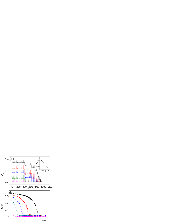
Figure 2: (Color online) For the same network used in Fig. 1, typical amplitude distributions observed in the first stage of the transition. (a) The distributions are generated by coupling strengths, from top to bottom, $\varepsilon=0.05,0.09,0.1,0.15,0.16$. Inset: The inverse relationship between the critical coupling $\varepsilon_{k}$ and the node degree $k$. The symbols are the numerical results, and the solid line is drawn by the theory. (b) For the same set of couplings as in (a), the averaged stair amplitude $\langle Z_{k}\rangle$ versus the node degree $k$. Each data of (b) is averaged over 50 network realizations.

To explore the staged transition and the stair structures appeared in Fig. 1, we proceed to investigate the system dynamics at the microscopic level. Specifically, we shall calculate the distribution of the node amplitude, $\{Z_{i}\}$, and see how this distribution is evolved during the transition. In the first stage, the node amplitude is evolved as follows. At very small coupling $\varepsilon\approx 0$, all nodes own the same amplitude $Z_{i}=r$, regardless of the difference of the node degree. Then, as $\varepsilon$ increases, all the amplitude will be decreased, but with very different speed. Specifically, the decrease of the amplitude of a node is proportional to the node degree. So the amplitude distribution is gradually curved and replaced by a non-smooth “stair-like” distribution, say, for example, the one generated by $\varepsilon=0.05$ in Fig. 2(a). In this stair-like distribution, nodes of the same degree will present the same amplitude, except some rare “bursts” which are caused by synchronous clusters (to be explained later). Because of the heterogenous degree distribution, the stairs are of different length. More interestingly, the height of the stairs is gradually stepping down with the node degree. That is, the highest stair consists of only the smallest-degree nodes and the lowest stair consists of only the largest-degree nodes. Increasing $\varepsilon$ further, the amplitude of the largest-degree nodes is hardly decreased, while the amplitude of the other nodes will be decreased continuously. This results a hierarchical death of the amplitude stairs. The process of stair elimination is shown in Fig. 2(a), where some typical amplitude distributions observed in the first stage are presented. Finally, at about the coupling strength $\varepsilon^{\prime}$, the last stair, i.e. the stair consisting of the smallest-degree nodes, will be eliminated, and the first-stage transition is completed. For instance, the distribution generated by $\varepsilon=0.16$ in Fig. 2(a). So the stair structures appeared in Fig. 1(b) is just a reflection of the hierarchical death of the amplitude stairs.

The formation of amplitude stairs could be analyzed by the mean-field approximation. Noticing that Eq. (1) can be rewritten as $\dot{Z_{i}}(t)=[(r^{2}-\varepsilon k_{i})+i\omega_{i}-|Z_{i}|^{2}]Z_{i}(t)+G_{i}$, where $G_{i}=\varepsilon\sum_{j=1}^{N}a_{ij}Z_{j}$ is the collective coupling received by node $i$. When $\varepsilon$ is small, most oscillators of the network will behave incoherently, therefore $G_{i}$ is small and negligible to the node dynamics, especially for the large-degree nodes. With this concern, the node dynamics can be simplified to $\dot{Z_{i}}(t)=[(r^{2}-\varepsilon k_{i})+i\omega_{i}-|Z_{i}|^{2}]Z_{i}(t)$. By requiring $|\dot{Z_{i}}(t)|=0$, we obtain

$$|Z_{i}|^{2}=r^{2}-\varepsilon k_{i}.$$ (2)

Eq. (2) tells that, for a given coupling strength, the amplitude of a node is only dependent on the node degree. This explains why the height of the stairs in Fig. 2(a) is decreased with the node degree. From Eq. (2) we can also estimate the averaged amplitude of each stair $Z_{k}$, which is verified by the numerical data of Fig. 2(a). Moreover, by setting $|Z_{i}|=0$ in Eq. (2), we can obtain the critical coupling $\varepsilon_{k}$ where the $k$-degree stair is eliminated: $\varepsilon_{k}\approx r^{2}/k$. The inverse relationship between $Z_{k}$ and $k$ is verified in the inset plot of Fig. 2(a).

It should be mentioned that the above analysis works for only the case of weakly coupled networks. If the coupling strength is not too weak, some nodes in the network could behave coherently. In such a case, the value of $G_{i}$ will be deviated from $0$, and the flat stairs predicted by Eq. (2) will be disturbed. This is just we have observed in simulations. In Fig. 2(a), despite the changes of the coupling strength, there always exist some bursts in the distributions. These bursts, which have random locations and various amplitude, are directly resulted from the synchronized nodes. The picture is the following. Since the node frequency is randomly chosen, there could be the situation that some connected nodes in the network have very small frequency mismatch. As the coupling strength increases, these nodes will be easily synchronized and form some synchronous clusters (phase synchronization PS ). Once synchronized, nodes will be efficiently protected from AD PAD:LATTICE ; AD:RING , showing as the amplitude bursts. The synchronized nodes, however, may have different amplitude, as they could be embraced by different set of neighbors. To smooth the amplitude bursts caused by synchronization, we have calculated the averaged stair amplitude, $\langle Z_{k}\rangle$, as a function of $k$. Now a smooth, hierarchical transition of AD is presented [Fig. 2(b)].

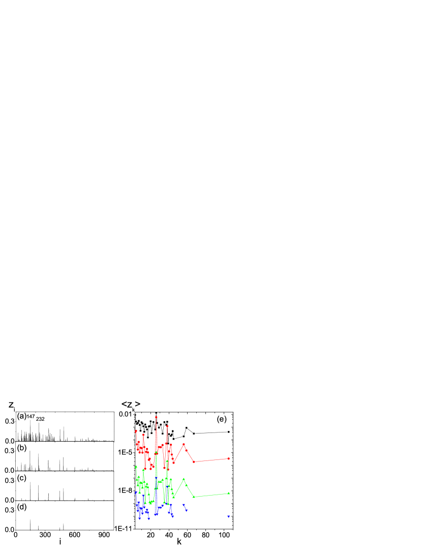
Figure 3: (Color online) For a slightly modified network model, the amplitude distributions observed in the second and third stages of the transition. (a) $\varepsilon=0.18$ and (b) $\varepsilon=0.19$ are within the second stage. (c) $\varepsilon=0.21$ and (d) $\varepsilon=0.22$ are within the third stage. (e) For the above amplitude distributions, the variations of $\langle Z_{k}\rangle$ as a function of $k$. The missed data in the last distribution is caused by the limited computing precision.

We go on to investigate the transition in the second stage. At the end of the first stage, a number of synchronous clusters are formed in the network. Because of synchronization, the amplitude of the synchronized nodes are apparently larger than the non-synchronized ones. In the second stage, as the coupling strength increases, both the number and the size of the synchronous clusters are decreased. Interestingly, it is found that the robustness of a cluster is mainly determined by the frequency mismatch between the synchronized nodes, while is less affected by the node degree or cluster size. To show this point more clearly, we have slightly modified the network by artificially adjusting the frequency mismatch between two connected nodes, $(147,232)$, to be $\delta\omega=1\times 10^{-3}$. This pair of nodes, both having the smallest degree $k_{min}=3$, are synchronized at a very small coupling and are kept at large amplitude till the very end of the transition. As shown in Fig. 3, despite of the increase of the coupling strength, the amplitude of these two nodes is always apparently larger than the resting nodes. Different to the situation of the first stage, in the second stage the node amplitude is less dependent of the node degree, as indicated by Fig. 3(e).

The second-stage transition is ended up with a state of very few synchronous clusters. Typically, each cluster consists of only several nodes which have very close natural frequencies, like the pair of nodes discussed above. The few survival clusters, however, are extremely robust and could stand for a very large coupling strength. The robust clusters result the new form of transition in the third stage: A fast death of the non-synchronized nodes accompanied by a slow death of the synchronized nodes. This property of network transition can be read from Fig. 3(b) and (c), where the amplitude of nodes $147$ and $232$ are kept at large values, while the amplitude of the other nodes is extremely small (see also Fig. 3(e)). Like the second stage, in the third stage the node amplitude is also less dependent on the node degree, as can be found from Fig. 3(e). With the elimination of the most robust cluster, the whole transition is completed.

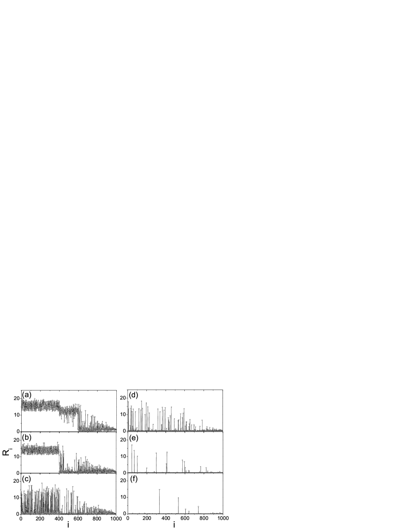
Figure 4: Typical amplitude distributions ($R_{i}=\langle\sqrt{x_{i}^{2}(t)+y_{i}^{2}(t)}\rangle$) observed in the transition of the network of chaotic Rössler oscillators. (a) $\varepsilon=0.039$ and (b) $\varepsilon=0.05$ are within the first stage; (c) $\varepsilon=0.055$ and (d) $\varepsilon=0.06$ are within the second stage; and (e) $\varepsilon=0.065$ and (f) $\varepsilon=0.07$ are within the third stage.

Whether the above phenomena about AD transition can be found for the general dynamics, say, for example, chaotic oscillators? To answer this, we have checked the transition of the same network but for chaotic Rössler oscillators. The dynamics of a single oscillator is described by $F_{i}(\textbf{x})=[-\omega_{i}y_{i}-z_{i},\omega_{i}x_{i}+0.165y_{i},z_{i}(x_{i}-10)+0.2]$, where $\omega_{i}$ is the natural frequency of the $i$th oscillator. In simulation, $\omega_{i}$ is chosen randomly from the range $[1,3]$. The coupling function is $H(\textbf{x})=x$. Fig. 4 is a collection of the amplitude distributions observed during the transition, which repeat the phenomena of Landau-Stuart oscillators. Besides the specific network in Fig. 1, we have also tested the transition to CAD in other networks, including changing the network size and the degree distribution, adopting the clustered networks, and considering the degree assortativity. The general finding is that, given the degree distribution is heterogeneous, the phenomena of staged transition and stair structures will be presented.

To summarize, we have studied the transition to CAD in scale-free networks of nonlinear oscillators, and found the important role of node degree played in AD generation. Since many practical systems where AD is importantly concerned possess heterogeneous degree distribution, our findings might give some new thoughts to the relevant studies, say, for example, the stability and evolution of ecological networks MRM:2001 ; ECOSYS .

XGW is supported by the National Natural Science Foundation of China under Grant No. 10805038.

References

- (1) D.J. Watts and S.H. Strogatz, Nature 393, 440 (1998).
- (2) A.-L. Barabási and R. Albert, Science 286, 509 (1999).
- (3) R. Albert and A.-L. Barabási, Rev. Mod. Phys. 74, 47 (2002); M.E. Newman, SIAM Rev. 45, 167 (2003).
- (4) S. Boccaletti, V. Latora, Y. Moreno, M. Chavez, and D.-U. Hwang, Phys. Rep. 424, 175 (2006); S. Boccaletti and L.M. Pecora, Chaos 16, 015101 (2006); J.A.K. Suykens and G.V. Osipov, Chaos 18, 037101 (2008).
- (5) X. F. Wang and G. Chen, Int. J. Bifurcation Chaos Appl. Sci. Eng. 12, 187 (2002); M. Barahona and L. M. Pecora, Phys. Rev. Lett. 89, 054101 (2002).
- (6) A. E. Motter, C. S. Zhou, and J. Kurths, Europhys. Lett. 69, 334 (2005); X.G. Wang, Y.-C. Lai, and C.H. Lai, Phys. Rev. E 75, 056205 (2007).
- (7) Y. Yamaguchi and H. Shimizu, Physica (Amsterdam) 11D, 212 (1984); K. Bar-Eli, Physica D 14, 242 (1985); R.E. Mirollo and S.H. Strogatz, J. Stat. Phys. 60, 245 (1989); D.G. Aronson, G.B. Ermentrout, and N. Kopell, Physica (Amsterdam) 41D, 403 (1990); G.B. Ermentrout, Physica (Amsterdam) 41D, 219, (1990).
- (8) D.V. Ramana Reddy, A. Sen, and G.L. Johnston, Phys. Rev. Lett. 80, 5109 (1998); Physica (Amsterdam) 129D, 15 (1999); Phys. Rev. Lett. 85, 3381 (2000).
- (9) F.M. Atay, Physica (Amsterdam) 183D, 1 (2003); Phys. Rev. Lett. 91, 094101, (2003).
- (10) S.H. Strogatz, Nature (London) 394, 316 (1998).
- (11) R. Herrero, M. Figueras, J. Rius, F. Pi, and G. Orriols, Phys. Rev. Lett. 84, 5312 (2000); D.V. Ramana Reddy, A. Sen, and G.L. Johnston, Phys. Rev. Lett. 85, 3381 (2000).
- (12) D.V. Ramana Reddy, A. Sen, and G.L. Johnston, Phys. Rev. Lett. 80, 5109 (1998); M. Wei and J. Lun, Appl. Phys. Lett. 91, 061121 (2007).
- (13) M.F. Crowley and I.R. Epstein, J. Phys. Chem. 93, 2496 (1989); M. Yoshimoto, K. Yoshikawa, and Y. Mori, Phys. Rev. E 47, 864 (1993).
- (14) L. Rubchinsky and M. Sushchik, Phys. Rev. E 62, 6440 (2000).
- (15) J. Yang, Phys. Rev. E 76, 016204 (2007).
- (16) Z. Hou and H. Xin, Phys. Rev. E 68, 055103(R) (2003).
- (17) M.G. Rosenblum, A.S. Pikovsky, and Jurgen Kurths, Phys. Rev. Lett. 76, 1804 (1996).
- (18) R.M. May, (2001) Stability and Complexity in Model Ecosystems. Princeton Landmarks in Biology. Princeton: Princeton University Press, (2001).
- (19) J.M. Montoya and R. V. Solé, preprint cond-mat/0011195; Camacho, J.R. Guimerà , and L.A.N. Amaral, preprint cond-mat/0102127.