Synchronization mechanism of sharp edges in rings of Saturn

Abstract

We propose a new mechanism which explains the existence of enormously sharp edges in the rings of Saturn. This mechanism is based on the synchronization phenomenon due to which the epicycle rotational phases of particles in the ring, under certain conditions, become synchronized with the phase of external satellite, e.g. with the phase of Mimas in the case of the outer B ring edge. This synchronization eliminates collisions between particles and suppress the diffusion induced by collisions by orders of magnitude. The minimum of the diffusion is reached at the center of the synchronization regime corresponding to the ratio 2:1 between the orbital frequency at the edge of B ring and the orbital frequency of Mimas. The synchronization theory gives the sharpness of the edge in few tens of meters that is in agreement with available observations.

1 Introduction

Together with very small thickness, extreme sharp edges in rings of Saturn are one of the most outstanding features of planetary rings (see e.g. Fridman & Gorkavyi (1999); Esposito (2002, 2006); Borderis et al. (1982)). Indeed, for example the outer B ring edge has a density drop by an order of magnitude on a distance $r_{e}\sim 10m$ that is enormously sharp compared to the edge distance to Saturn ($117580km$), the B ring width ($25580km$) and the width of Cassini division ($4620km$). This is especially surprising since the life time of the rings is enormously large being of about $10^{12}$ orbital periods (Fridman & Gorkavyi, 1999) and the particles inside the B ring are quite dense (e.g. there are particles of size $10m$ down to $1cm$ and smaller with a distance between them of about a few meters and less) (Fridman & Gorkavyi, 1999; Esposito, 2002, 2006; Spahn & Schmidt, 2006). Due to this about $10-100$ collisions between particles per orbit should wash out all sharp density contrasts in only a few orbital periods.

In many cases, and perhaps always, these sharp edges are associated with the gravitational perturbation by a moon inside or outside the rings. The abruptness of the transition from nearly opaque to practically transparent regions was constrained by the Voyager Photopolarimeter data (Lane et al., 1982) to be smaller than about 100 meters. Cassini UVIS occultation profiles show edges sharper than tens of meters, and in fact the assumption of a knife-edge sharpness is used to constrain the local ring thickness near the edge to be on the order of 5 meters only ((Colwell et al., 2008, 2009); ring thickness and sharpness of the edge should be of the same order).

After the pioneering work of Wisdom & Tremaine (1988) extensive numerical simulations of particle dynamics have been performed by different groups (see e.g. Salo (1995); Lewis & Stewart (2000); Seiss et al. (2005); Charnoz et al. (2007); Sremcevic et al. (2007)) that allowed to establish a number of interesting properties of ring dynamics. However, the problem of sharp ring edges still remains a mystery. Its solution requires extensive large scale numerical simulations with particles of different scales, it also may require to go beyond local box simulations invented by Wisdom & Tremaine (1988). In view of these difficulties it seems to be useful to explore certain simplified models that bring to surface new qualitative physical effects which can be analyzed more directly due to model simplicity. Here, we introduce such a simplified model of ring dynamics for outer B ring edge called the SYNC model in the following. Numerical investigations of this model show a striking phenomenon of synchronization of the epicycle motions of particles in the ring induced, under certain conditions, by a periodical gravitational force of Mimas. In a general context, the synchronization phenomenon, which has abundant manifestations in science, nature, engineering and social life (Pikovsky et al., 2001; Strogatz, 2003), can be roughly described as an adjustment of frequencies and phases of oscillators due to interaction and/or forcing. In the present context, the phases of the epicycle rotation of various particles become synchronized with the phase of periodic gravitational force of Mimas, and as a result the collisions between particles become suppressed by orders of magnitude so that the diffusion in the ring also becomes suppressed by orders of magnitude. This leads to a maintaince of sharp edges in a certain frequency range of ratios of epicycle frequency $\Omega$ to the Mimas frequency $\omega$. We note that the data of the Cassini mission show that the outer B ring edge has the frequency $\Omega_{B}$ which is very close to $2:1$ resonance with Mimas frequency $\omega$, actually $(\Omega_{B}-\Omega_{S})/2\omega=\Omega_{B}/2\omega-1\sim 10^{-5}-10^{-4}$ that corresponds to the accuracy in coordinate position of about $1$ to $10km$. Thus $\Omega_{B}$ is located directly in the middle of the synchronization Arnold tongue where the synchronization effects are the strongest. As a noticeable remark we mention, that it was Christiaan Huygens who discovered both the Saturn’s rings (see, e.g. references in book (Fridman & Gorkavyi, 1999)) and the synchronization phenomenon (see, e.g. references in book (Pikovsky et al., 2001)).

The paper is composed as follows: the SYNC model of dynamics in the ring is described in Section 2 (with additional details given in Appendix A, B), the numerical and analytical results are presented in Section 3, the discussion of the results is given in Section 4.

2 Description of the SYNC Model of Ring Dynamics

The SYNC model of the ring dynamics is based on the four main ingredients:

1. the individual particle dynamics is given by the Hill equations and is considered in a local box as it is proposed by Wisdom & Tremaine (1988), the particles are assumed to be identical, the dynamics is considered only in the two-dimensional plane of the ring;

2. the gravitational force of Mimas is considered as a sequence of periodic kicks of fixed amplitude;

3. the collisions between particles are treated on the basis of the mesoscopic multi-particle collision model proposed by Kapral (see e.g Malevanets & Kapral (2004));

4. the total energy balance (the process where the injection of energy provided by the shear flow (Wisdom & Tremaine, 1988) and the gravitational force of Mimas is equilibrated by dissipation) is ensured via the Nosè-Hoover thermostat which is broadly used in molecular dynamics simulations of large ensembles of interacting particles (see e.g Hoover (1999); Rateitschak et al. (2000); Hoover et al. (2004)).

Let us now describe the elements of the model in more details:

(i) The Hill equations of motion inside a local box (Wisdom & Tremaine, 1988) are

$$\begin{array}[]{ll}\dot{x}=v_{x};\;\;\dot{y}=v_{y}+V_{s};\;\;\dot{v}_{x}=2\Omega v_{y}+F_{x}(t)/m_{p};\\ \dot{v}_{y}=-\Omega v_{x}/2;\;\;V_{s}=-3\Omega x/2.\end{array}$$ (1)

where $\Omega=\sqrt{GM_{Saturn}/a_{0}^{3}}$ is the Kepler frequency of a particle of mass $m_{p}$, $V_{s}$ is the Kepler shear velocity, $F_{x}(t)$ is the gravitational force of Mimas along axis $x$ directed to Saturn. Here $v_{x},v_{y}$ are velocities of local motion in the presence of the shear flow. With $GM_{Saturn}=3.79\times 10^{16}m^{3}/s^{2}$ and the radius $a_{0}=1.17\times 10^{8}m$ we have at the edge of B ring $\Omega=\Omega_{S}=1.52\times 10^{-4}s^{-1}$. We normalize all velocities by a typical value of epicycle velocity $v_{ep}=0.005m/s$ that gives us equations of motion in a dimensionless form. After that the distance is measured in units of a typical epicycle radius $r_{s}=v_{ep}/\Omega_{S}=32.7m$ and time $t$ is replaced by $\Omega_{S}t$. The local box has the periodic boundary conditions as those used by Wisdom & Tremaine (1988). The size of the box is usually taken as a square $S=5r_{s}\times 5r_{s}$. In presence of the Nosè-Hoover thermostat (see (iv)) and the shear flow we found convenient to use the Hamiltonian form of the Hill equations as it is described by Stewart (1991). In this formulation the Hamiltonian of the epicycle motion has the form $H_{ep}=\Omega I=(v_{x}^{2}+v_{y}^{2})/2$ where $I$ is the action of the oscillator motion. More details are given in Appendix A.

(ii) The computation of the field strength $F_{x}$ is described in Appendix B. Because Mimas passes the local box rather fast, the force in dimensionless units has a form of periodic delta-function $f(t)=F_{x}(t)/(m_{p}v_{ep})=\epsilon\sum_{l}\delta(t-l\tau_{M})$ with the period $\tau_{M}$ defined by the dimensionless orbital period of Mimas $\tau_{M}=2\pi\Omega_{S}/\omega$ and dimensionless kick strength $\epsilon=0.64$ corresponding to the fixed choice of the typical epicycle velocity $v_{ep}=0.005m/s$. The force in $y$-direction is neglected since it is much smaller compared to the force in $x$-direction and gives a small change of $v_{y}$ compared to the shear velocity.

(iii) The collisions of particles are performed according to the Kapral algorithm (Malevanets & Kapral, 2004). Namely, the whole local box $S$ is divided on $N_{cel}$ cells. Usually we use about $100\times 100$ cells with the total number of particles $N=1000$ corresponding to $N_{ep}=\pi r_{s}^{2}N/S\approx 125$ particles inside one epicycle circle and the particle density in a cell being $0.1$. After a time $\tau_{K}$ the relative velocities (with respect to the motion of the center of mass of the cell) of all particles in a given cell are rotated by a random angle. In this way the total momentum and energy inside a given cell are preserved while the directions of the velocities become mixed. It is important to note that during the collision the velocities inside the cell are taken as the total physical velocities of particles, namely ${\dot{x}},{\dot{y}}$ including the shear velocity. Thus, due to a finite size of the Kapral cells, the shear velocity always generates appearance of a spreading of local velocities $v_{x},v_{y}$: even if $v_{x}$ and $v_{y}$ of two particles coincide before the “collision”, this is not true for the total velocities ${\dot{x}},{\dot{y}}$, and random rotation of the latter leads to the appearance of non-equal $v_{x},v_{y}$. In a certain sense the finite size of Kapral cells physically acts as a finite size of colliding bodies. Usually we used $\tau_{K}=0.5/\Omega_{S}$ but the variation of this parameter did not affect the main results.

(iv) In presence of collisions the shear flow and the driving Mimas force inject additional energy in the system, that is dissipated via different mechanisms, including nonelasiticity of collisions, interactions with dust, etc. In our simplified model, to keep the energy balance, we use the Nosè-Hoover thermostat which is commonly used for molecular dynamics simulations of interacting particles, also in presence of external fields (Hoover, 1999; Rateitschak et al., 2000; Hoover et al., 2004; Chepelianskii et al., 2007). In this thermostat, which mimics a canonical ensemble, an additional friction force acts on a particle $i$ according to

$$\mathbf{\dot{p}}_{i}=\mathbf{F}_{i}-\gamma\mathbf{p}_{i}\;,\;\mathbf{\dot{q}}_{i}=\mathbf{p}_{i}\;,\,\\ \dot{\gamma}=[\langle\mathbf{p}^{2}\rangle/(2m_{p}T)-1]/{\tau_{H}}^{2}$$ (2)

where $\mathbf{p}_{i}\mathbf{q}_{i}$ are the momentum and coordinate of particle $i$, $\mathbf{F}_{i}$ is an effective “friction” force acting on a particle due to collisions and external fields, $\tau_{H}$ is the relaxation time in the NH thermostat [usually we used $\Omega_{S}\tau_{H}=16$ but we also checked that the variation of $\tau_{H}$ does not affect the synchronization phenomenon (see examples below)] and $\langle\mathbf{p}^{2}\rangle$ means the average over all $N$ particles, $T=m_{p}v_{ep}^{2}/2$ is a given temperature of the thermostat. One can see that the “friction” changes the sign with $\gamma$, and the variable $\gamma$ is driven by the deviations of the mean kinetic energy from that at the given temperature $T$, in this way the system is kept near this temperature as it should be for the canonical ensemble.

For the Hamiltonian form of the Hill equations, the friction acts only on the action variable that gives in dimensionless variables ${\dot{I}_{i}}=-\gamma I_{i},\dot{\gamma}=[\langle\mathbf{I}\rangle-1]/{\tau_{H}}^{2}$, where $\langle\mathbf{I}\rangle$ means the averaging over all $N$ particles (see Appendix A). The physical origin of the appearance of such an effective friction can be attributed to an average friction force acting on a relatively large particle as a result of multiple collisions with a dust of small size particles.

In a ring with extended size distribution the smaller particles have in equilibrium generally larger dispersion velocities (Salo, 1992). Since the collisions are inelastic, the system does however not assume a state of energy equipartition. Typically, the dispersion velocity of the smallest particles is by a factor of several larger than the one of the largest particles, depending mildly on the width of the size distribution and the inelasticity of the particles.

At opposition the perturbing moon induces an equal excess velocity $\Delta v_{x}$ to all ring particles, regardless of their size. This means that compared to collisional equilibrium the large particles have now a higher excess in random kinetic energy than the small ones. In this sense the return to equilibrium, mediated by dissipative collisions, affords a cooling of the large particles relative to the small ones, and thus, an effective friction on large particles. This friction vanishes in equilibrium like the Nose-Hoover thermostat. Large particles determine the dynamical properties of the ring.

Another dissipative process could be an ongoing exchange of ring-matter between particles of all size groups due to a balance of coagulation and fragmentation (dynamic ephemeral bodies, DEB’s, (Davis et al., 1984)) causing an effective dissipation, since the composition and destruction of agglomerates are irreversible processes.

It is interesting to note that the epicycle dynamics is rather similar to motion of charged particles in a magnetic field (Fridman & Gorkavyi, 1999) and due to that there is a certain analogy with the synchronization of the Larmor motion for two-dimensional electron gas in magnetic and microwave fields as it was discussed by Chepelianskii et al. (2007). The main difference to the present problem is that for the electron gas there is no shear.

3 Numerical results and their interpretation

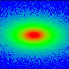
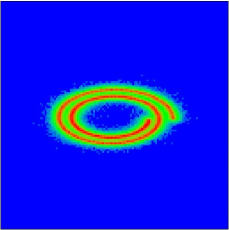
Figure 1: Density distribution of particles in the ring in the plane of local epicycle velocities $(-3<v_{x}/v_{ep}<3;-3<v_{y}/v_{ep}<3)$ obtained by the numerical simulations with $N=1000$ particles inside the spacial square box $S=5r_{s}\times 5r_{s}$ where $r_{s}$ is the epicycle radius; the particle density is $\rho=N_{p}/S=40/r_{s}^{2}$. The rotation frequency ratio is $\Omega/\Omega_{s}=\Omega/2\omega=1.15$ (left panel) and 1 (right panel, synchronized regime); the dimensionless force amplitude of Mimas is $\epsilon=0.64$. The number of Kapral cells is $N_{cel}=100\times 100=10^{4}$, the Kapral collisions are done after time $\tau_{K}=0.5/\Omega_{s}$; the relaxation time of Nosè-Hoover dynamics is $\tau_{H}=16/\Omega_{s}$. The data are averaged over time interval $0\leq t\leq 10^{4}/\Omega_{s}$. Density is proportional to color (red/gray for maximum, blue/black for minimum).

The results of numerical simulations for the particle density distribution in the plane of local epicycle velocities $(v_{x},v_{y})$ are shown in Fig. 1 for two values of $\Omega/2\omega$ ratio between the epicycle frequency of particles $\Omega$ and the double frequency of Mimas $2\omega$. For $\Omega/2\omega=1.15$ the distribution of velocities is close to the Maxwell distribution of elliptical form appearing due to shear and ellipticity of motion given by the Hill equations (the distribution becomes close to a symmetric one in rescaled velocities $\tilde{v}_{y}=2v_{y},{\tilde{v}}_{x}=v_{x}$). The distribution is drastically changed for $\Omega/2\omega=\Omega_{S}/2\omega=1$ : almost all density is concentrated on a spiral in the velocity plane. The physical meaning of this phenomenon is the following: for the resonant ratio $\Omega/2\omega=1$ the phases of the epicycle rotations become synchronized with the phase of periodic Mimas kicks given by $f(t)$. While out of the resonance (e.g. $\Omega/2\omega=1.15$) all epicycle phases are random and independent, in the synchronization regime they are all adjusted to the phase of Mimas. As a result, Mimas gives a kick in $v_{x}$, between kicks the particle velocity decreases doing two rotations over the spiral, then again it is kicked by Mimas in the same state as at previous kick, and so on. Thus the phases of this rotational motion are equal to the phase of Mimas and equal to each other. This means that the particles rotate in synchrony, at each moment of time their rotational velocities are equal both in the amplitude and in the direction. Therefore, the collisions between them effectively disappear. There remains only a residual relative velocity, related to the shear velocity and a finite size of the Kapral cells (finite size of colliding bodies in the ring). In the absence of shear flow the synchronization can be complete for all particles as it has been discussed by Chepelianskii et al. (2007) for the problem of two-dimensional electron gas in magnetic and microwave fields.

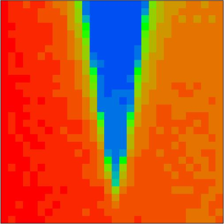
Figure 2: Dependence of the rescaled diffusion rate $D/{\tilde{D}}_{0}$ shown by color on the rescaled frequency $\Omega/2\omega$ (horizontal axis) and driving force strength $\epsilon$ (vertical axis) for the range $0.85\leq\Omega/2\omega\leq 1.15$ and $0\leq\epsilon\leq 0.7$. The color is proportional to $D/{\tilde{D}}_{0}$ with red/gray for maximum value ($D/{\tilde{D}}_{0}=1.26$) and blue/black for minimum ($D/{\tilde{D}}_{0}=4\times 10^{-4}$), here ${\tilde{D}}_{0}$ is the diffusion rate at $\epsilon=0,\Omega=\Omega_{s}$ (also $D/D_{0}=1.7\times 10^{-5}$ with $D_{0}=r_{s}^{3}\Omega_{s}$). Data are obtained for time $t\leq 10^{4}/\Omega_{s}$, $N=1000$, $N_{cel}=200\times 200$, other parameters are as in Fig.1.

Since the collisions are significantly reduced for the synchronization regime, the diffusion rate $D=\langle x^{2}\rangle/t$ is also reduced by orders of magnitude compared to its typical value $D_{0}=r_{s}^{2}\Omega_{S}$. This is clearly seen in Fig. 2 which gives the dependence of $D$ on $\Omega$ and $\epsilon$. The diffusion suppression takes place inside the Arnold tongue where the epicycle rotation is synchronized with the Mimas phase. According to the data of Fig. 2 the synchronization takes place inside the frequency range

$$|\Omega/2\omega-1|\leq s\epsilon$$ (3)

with the numerical value of the constant $s\approx 0.08$. According to the synchronization theory (Pikovsky et al., 2001) the synchronization region is given by the dimensionless amplitude of the driving force which is $2\epsilon/(4\pi\text{max}(v_{x}))$ that gives $s\approx 0.08$ since we have $\text{max}(v_{x})\approx 2$ (see Fig. 1). Thus the numerical dependence is in agreement with the analytical synchronization theory. The variation of $\Omega$ is related to the position of particle inside the ring. For example, $\Omega/2\omega=1.05$ corresponds to the distance $\Delta x\approx 3a_{0}(\Omega/2\omega-1)/2\approx 9000km$ from the outer B edge in direction to Saturn. It is interesting to note that this is of the order of the size of Cassini division.

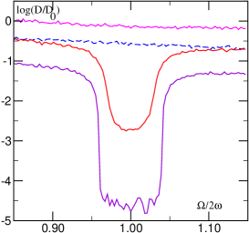
Figure 3: Dependence of the rescaled diffusion rate $D/D_{0}$ on the rescaled frequency $\Omega/2\omega$. The full curves are for $\epsilon=0.64$ with $N_{cel}=50\times 50,100\times 100,200\times 200$ from top to bottom; the dashed curve is for $\epsilon=0$ and $N_{cel}=100\times 100$. Data are obtained for time $t\leq 10^{4}/\Omega_{s}$, $N=1000$. Logarithms are decimal.

An interesting property of the relation (2) is its independence of the relaxation time scale $\tau_{H}$. Physically, this means that $\tau_{H}$ only determines the time scale on which the synchronization is reached but it does not affect the domain of synchronization. This is in agreement with our numerical checks which show that at the Mimas value of $\epsilon=0.64$ the synchronization window shows less than $10\%$ variation when $(\Omega_{S}\tau_{H})^{2}$ varies from $0.1$ to $10^{-5}$. For $(\Omega_{S}\tau_{H})^{2}=1$ this window is increased by about 30%.

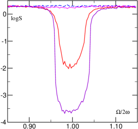
Figure 4: Dependence of the synchronization parameter $S$ on the rescaled frequency $\Omega/2\omega$. Parameters are the same as in Fig.3. Logarithms are decimal.

The variation of the diffusion rate $D(\Omega)$ when the number of Kapral cells $N_{cel}$ is changed is shown in Fig. 3. For $N_{cel}=50\times 50$ the collisions happen rather often and there are no signs of synchronization. For $N_{cel}=100\times 100$ the synchronization sets in and the diffusion drops inside the synchronization window. A further increase up to $N_{cel}=200\times 200$ gives much stronger drop of the diffusion inside the synchronization window while its size is only slightly increased. Outside of this window the diffusion scales as $D\propto 1/N_{cel}$. This is rather natural since $D$ is proportional to the density of particles inside the cell so that $D\sim r_{s}^{2}\Gamma\sim r_{s}^{2}N/(N_{cel}\tau_{K})$ where $\Gamma$ is the effective collision rate. We note that in the non-synchronized regime the diffusion rate per orbital period is rather large being $2\pi D/(r_{s}^{2}\Omega_{S})\approx 3$ (at $N_{cel}=100\times 100$) and 1 (at $N_{cel}=200\times 200$). These values approximately correspond to the typical conditions for particles inside B ring.

Another signature of synchronization can be expressed via        the synchronization parameter        $S=\sum_{i<j}(\mathbf{v}_{i}-\mathbf{v}_{j})^{2}/(N^{2}v_{ep}^{2}/2)$. Its dependence on frequency is shown in Fig. 4. Inside the synchronization regime $S$ drops by almost 4 orders of magnitude. This means that due to synchronization the relative collision velocities of particles are very small and therefore the diffusion is also very small. At the same time the velocity difference remains finite due to finite size of the cells (collision bodies) and the shear flow. In absence of the shear flow the collisions disappear completely (see also (Chepelianskii et al., 2007)).

For the chosen value $v_{ep}=0.005m/s$ we have $\epsilon=0.64$ (see Appendix B) that according to (2) and the data of Figs. 2,3,4 give the synchronization border $\Omega/2\omega\approx 1.05$. This corresponds approximately to $x_{S}=9000km$ distance from the exact resonance 2:1. The observations give this distance to be about $x_{B}\approx 1-10km$ that is significantly smaller than the synchronization border. Of course, the value of $v_{ep}$ is not known exactly and may be a factor $2$ to $10$ different from the value chosen above. But even if the actual value is 10 times larger than still $x_{S}$ remains by 2 orders of magnitude larger than the observed B edge position $x_{B}$.

\psfrag{xlabel}[c][c]{position $x/r_{S}$}\psfrag{ylabel}[c][c]{time $\Omega_{s}t$}\includegraphics[width=239.00298pt]{fig5.eps}

Figure 5: Dependence of density of particles (in arbitrary units) on time $\Omega_{S}t$ (vertical axis) and position in the ring $x/r_{S}$ (horizontal axis) for $\epsilon=0.6$, $\Omega/2\omega=1.1$ and zero frequency gradient $g=0$.. There are $N_{cel}=1200\times 120$ in the whole space box $S=50r_{S}\times 5r_{S}$; $\tau_{K}=0.5/\Omega_{s}$, $\tau_{H}=4.5/\Omega_{S}$. Initially there are $N=60$ particles in the left box $S=5r_{S}\times 5r_{S}$ and this number is kept constant during the computations till the finite moment of time $\Omega_{S}t=6.28\times 10^{4}$ when there are 305 particles in total.

We explain this disagreement in the following way. Taking the value $\epsilon=0.64$ we assume that the particles appear initially in the non-synchronized part of the ring, let say with $\Omega/2\omega\approx 1.2$. Due to collisions these particles diffuse closer and closer to the synchronization border at $\Omega/2\omega\approx 1.05$. Behind this border the diffusion rate drops $D(\Omega)$ drastically due to the synchronization phenomenon described above. This sharp drop of $D$ creates a diffusive shock wave which continues to propagate slowly inside the synchronization region since there the diffusion remains finite due to the shear flow (see Figs. 2,3). The edge size of this diffusive shock wave should be of the size of few epicycle radius $r_{s}$ since as soon as the distance between particles becomes larger than $r_{s}$ the collisions between them completely disappear due to a frozen nature of epicycle motion (in a close similarities with particles in a magnetic field, see e.g. (Fridman & Gorkavyi, 1999)). In this way the gradient of density slowly moves inside the synchronization domain keeping the sharpness of the edge of a few epicycle radius $r_{s}$. In the synchronization domain the diffusion is minimal at the exact resonance $\Omega/2\omega=1$ since the synchronization effect is the most strong there (see Figs. 2,3,4). Therefore, the edge of synchronized particles spends the most of the time at that place with the minimum of diffusion. This is actually the place where the outer B ring edge is observed now.

\psfrag{xlabel}[c][c]{position $x/r_{S}$}\psfrag{ylabel}[c][c]{time $\Omega_{s}t$}\includegraphics[width=239.00298pt]{fig6.eps}

Figure 6: Dependence of density of particles (in arbitrary units) on time $\Omega_{S}t$ (vertical axis in logarithmic scale) and position in the ring $x/r_{S}$ (horizontal axis) for $\epsilon=0.6$, the frequency gradient in space is $g=0.002$ with $\Omega/2\omega=1.05$ at $x=0$ and $\Omega/2\omega=1$ at $x/r_{S}=25$ corresponding to the outer B ring edge. There are $N_{cel}=1200\times 120$ in the whole space box $S=50r_{S}\times 5r_{S}$ (only half is shown); $\tau_{K}=0.5/\Omega_{s}$, $\tau_{H}=4.5/\Omega_{S}$. Initially there are $N=60$ particles in the left box $S=5r_{S}\times 5r_{S}$ and this number is kept constant during the computations till the finite moment of time $\Omega_{S}t=6.28\times 10^{5}$ when there are 305 particles in total.

To give more justification to the above picture we performed extensive numerical simulations of front propagation of particles in the SYNC model. With this aim we introduced a gradient of the frequency $\Omega$ with the distance $x$ so that $\Omega(x)=\Omega_{0}-gx$ where $\Omega_{0}\approx 1.1$ is some initial value and $g\sim 0.002$ is the frequency gradient per unit of epicycle radius in dimensionless units. Examples of the numerical simulations are shown in Figs. 5,6. In the absence of the gradient, in the non-synchronized regime there is a diffusive spreading along $x$ as it is clearly seen in Fig. 5. The typical diffusive profile $x\propto\sqrt{t}$ is clearly seen. The computations are done at the fixed constant particle density $\rho$ in the left space box $5r_{S}\times 5r_{S}$ of the total longitudinal space box $S=50r_{S}\times 5r_{S}$ with the number of Kapral cells $N_{cel}=1200\times 120$. This is reached by adding new particles inside the left space box during the diffusive spreading. At such a density $\rho r_{S}^{2}=60/25$ and such a value $N_{cel}$, the local diffusion rate at $\Omega/2\omega\approx 1.1$ is $D/D_{0}\approx 0.01$ and during the time $\Omega_{S}t=6.28\times 10^{4}$ the diffusion propagates on a distance $x\approx\sqrt{Dt}\approx 25r_{S}$ that is in a good agreement with the data of Fig. 5.

\psfrag{xlabel}[c][c]{position $x/r_{S}$}\psfrag{ylabel}[c][c]{density}\includegraphics[width=239.00298pt]{fig7.eps}

Figure 7: Dependence of density of particles (arbitrary units in logarithmic scale) on position in the ring $x/r_{S}$ for $\epsilon=0.6$ at the final time $\Omega_{s}t=6.28\times 10^{4}$ (red/gray for parameters of Fig. 5) and $\Omega_{s}t=6.28\times 10^{5}$ (blue/black for parameters of Fig. 6).

The situation is drastically different in presence of the frequency gradient $g=0.002$ when the particles enter inside the synchronization window $\Omega/2\omega-1<0.05$ as it is shown in Fig. 6. Even if the total computation time here is 10 times larger than in Fig. 5 the front propagation becomes very slow around $x/r_{S}\approx 17$ since diffusion drops strongly inside the synchronization window going down to very small by finite value $D/D_{0}\approx 3\times 10^{-6}$ inside the left space box $5r_{S}\times 5r_{S}$ with $60$ particles.

Of course, the value of the gradient chosen here is much larger than its real value $g\sim 3r_{S}/2x_{s}\sim 15m/1.17\times 10^{5}km\sim 10^{-7}$. Such small values of the gradient are not accessible for nowadays computer simulations. However, a more smooth, adiabatic variation of the orbital frequency $\Omega$ on a scale of an epicycle radius should make the picture of the diffusive shock wave moving inside the synchronization domain to be even better justified.

The density $\rho(x)$ dependence on $x$ at a final moment of time (averaged over 1% of total time) is shown in Fig. 7. for the cases of Figs. 5,6. In the case of synchronization (Fig. 6) there is a sharp drop of density on a scale of 2 epicycle radius $r_{S}$. In the non-synchronized case (Fig. 5) the decrease of density goes in a more smooth way (on a scale of about $10r_{S}$). The difference of scales in two cases is not so large since in both cases the diffusion is zero in the region without particles. However, the most important difference is that the rapid diffusive propagation goes unlimitedly in the non-synchronized case while inside the synchronization window the propagation front moves very slowly with the formation of sharp density drop on a scale of about $2r_{S}$. The front stays the longest time at the place where the diffusion is minimal that corresponds to the center of the synchronization window at $\Omega=2\omega$. For the value of $r_{S}\propto 1/v_{ep}\approx 36m$ given above this gives the size of the edge $\Delta x_{e}\approx 2r_{S}\approx 70m$. This value is in a good agreement with the observation data which give $\Delta x_{e}\approx 10m$ especially if we take into account that the average value $v_{ep}$ is known only by an order of magnitude.

4 Discussion

Our studies based on the SYNC model of dynamics in the rings of Saturn show the emergence of synchronization in the vicinity of the outer B ring edge. Like the Maxwell demon this synchronization makes the epicycle motion of particles to be synchronous that practically eliminates collisions between them. This gives a suppression of diffusion by orders of magnitude and a formation of a diffusive shock wave slowly propagating inside the synchronization domain. The size of this front or the edge of the ring is of the order of a few epicycle radius being of about of a few tens of meters. This is in agreement with the present observation data which give its size to be about 10 meters. The size of the synchronization domain created by Mimas is of the order of $4000km$ (remarkably, the total number of synchronized particles, which can be estimated as $>10^{12}$, is huge). The front moves most slowly in the center of the synchronization domain so that it is most probable to observe it at the exact resonance 2:1 between the edge frequency and the frequency of Mimas. The observations show that the actual position is close to this value with a relative accuracy of $10^{-4}-10^{-5}$.

Similar synchronization effects should exist at other resonances with other satellites. Our preliminary data give a similar picture for the outer A ring edge which is closely located to the 7:6 resonance with Janus (here the dimensionless kick strength is $\epsilon\approx 1.19$ but the relative frequency size of the synchronization window is approximately twice smaller due to higher order of the resonance).

The synchronization mechanism proposed here can also be responsible for existence of very narrow planetary rings. Indeed, if initially particles are distributed inside the resonance then those which are inside the synchronization window will remain there practically forever since the collision induced diffusion is switched off, while those outside of the window will diffuse away living a narrow ring of particles inside the synchronization window.

The SYNC model used in this paper is based on several significant simplifications of the real particle dynamics. The use of the mesoscopic Kapral method for incorporating the collisions appears to imply no additional physical mechanisms, but the basic physics of the collisions remains hidden inside the parameters of the Kapral method - the number of the cells and the frequency of the reshuffling of velocities. To make the calculations more realistic, one needs to incorporate realistic collision models with reasonable mechanical properties of the particles, to include a distribution of the sizes, etc. Such an extension goes far beyond the scope of our preliminary study. Thus we can hardly make direct predictions, in particular, compare properties of A and B ring edges.

Moreover, it appears that another simplification of our computational model – the use of the Nosè-Hoover thermostat – is less “repairable” and requires a further justification. Indeed, if there is some average dissipation due to particle collisions, this justifies the use of the thermostat for modeling the saturation of the energy pumped to the system due to shear. On the other hand, in our setup in the synchronized state collisions are rare so at the first glance there is no mechanism for energy saturation. Here it is important to mention, that we restricted our analysis to an ensemble of identical particles. For a particular situation in the outer B ring this means that we consider only large particles that have low characteristic epicyclic velocities. If there is a whole range of particles of different sizes, they are all subject to resonant kicks by Mimas, but because their characteristic epicyclic velocities are different, the effect of the kicks is also different. If we assume rough equipartition of epicylic kinetic energies, then smaller particles have larger velocities, therefore for them the effective forcing parameter $\epsilon$ is smaller, and as a result they only weakly synchronize or not synchronize (if they lie near the bottom of Fig. 2). Collisions with these randomly moving particles may provide an additional dissipation that justifies the use of the Nosè-Hoover thermostat. Further investigations (which however go far beyond the scope of this paper) of different dissipation effects influencing the energy balance are needed to clarify this issue.

Another simplification made – a consideration of a relatively small box of particles – is also crucial. Indeed, parts of the ring at different angular coordinates are statistically equivalent, but the dynamical equivalence is broken by the influence of Mimas, as the latter kicks the particles at different phases. Thus the synchrony of the velocities may be only local, i.e. the velocities of particles are synchronized with the local phase of the Mimas, but this phase changes gradually along the ring angular coordinate. Because of the differential rotation, the particles synchronized at different phases will mix, but this effect is not taken into account in the box model, it has to be addressed in future studies.

In this respect the important issue is that of how the synchronization of particles’ velocities could be tested experimentally. Indeed, the theory above predicts a drastic narrowing of the width of the velocities distribution, cf. Fig. 1. However, because the velocities themselves are very small, there is no much hope to observe the distribution of them directly, e.g. by Doppler measurements or image analysis. Thus one has to rely on implicit observations. For example, one may expect that the adjustment of velocities influences other dynamical features recently observed in the rings, like propeller structures (Sremcevic et al. (2007); Spahn & Schmidt (2006)). However, for such an implicit test one has to find such structures quite near to the sharp edges described above. Remarkably, near the outer edge of ring B a scrambled pattern is observed in recent Cassini images ( see URL: http://saturn.jpl.nasa.gov/photos/imagedetails/ index.cfm?imageId=2984 ) that is probably due to a gravitational clumping of particle (cf. simulations by Lewis & Stewart (2005) of a similar structure at the Encke gap). We can speculate that the synchronization of large particles would generally enhance their ability to clump due to gravitational and adhesive forces, because their relative collision velocities become rather small. On the other hand, if smaller, non-synchronized particles, leave the ring and enter the gap, where large particles are missing, their diffusion will be reduced as well, because the collisions between small particles are rare. Observation of such a gradient in the size distribution of particles near the edge may also be interpreted as an implicit confirmation of the suggested mechanism.

We note that in the literature several mechanisms for explanation of sharp edges of rings have been discussed. One process to form and maintain a sharpness is a shear reversal induced by a strong gravitational perturbation near a resonance with a moon. In the unperturbed ring Keplerian shear leads to an outward viscous transport of angular momentum. The distortions induced by a perturber may locally reverse the shear and, when integrating over the azimuth, to a net angular momentum transport that is directed radially inward (Borderis et al., 1982, 1983, 1989; Mosqueira, 1996). This process can lead to an inward migration of material from the close vicinity of the resonance location with the moon, and in this way clear a gap at this radial position in the ring. Recently Lewis et al. reported on a “negative diffusion” mechanism, where the particles migrate to areas of high density (Leezer & Lewis (2006)). In their calculations, however, only a single pass by the moon was simulated so no resonant effects, like those we focus on in this study, were possible. Probably, further observations, together with further extensive numerical simulations, will allow one to test which mechanism is responsible for the sharp edges of the rings. It appears highly desirable to compare various setups in numerical simulations as well.

Finally, we note that, as discussed by Chepelianskii et al. (2007), the elimination of collisional diffusion may appear also for charged particles in a magnetic field like 2D electron gas (see Mani et al. (2002); Zudov et al. (2003)) and electron and ion clouds in a Paul trap (see, e.g., Mortenson et al. (2006)). Due to that it can be rather interesting to try to make laboratory experiments with traps (see e.g. Major et al. (2005)) which would allow to model rings of Saturn in laboratory experiments with cold ions.

Appendix A The Hamiltonian form of the Hill equations

Here we describe the Hamiltonian form of the Hill equations. According to Stewart (1991), the Hill equations (1) can be viewed as a Hamiltonian system with

$$H=\frac{1}{2}[(p_{x}+\Omega y)^{2}+(p_{y}-\Omega x)^{2}]-\frac{3}{2}\Omega^{2}x^{2}-xF_{x}(t)/m_{p}$$ (4)

For the simulation and the analysis another representation, also given by Stewart (1991), where the epicyclic and shear motion are effectively separated, is more convenient. One introduces canonical variables $I,\phi,P,Q$ according to

$$x =\frac{2}{\Omega}P-\sqrt{\frac{2I}{\Omega}}\cos\phi,\qquad y=Q+2\sqrt{\frac{2I}{\Omega}}\sin\phi$$ (5)

$$\dot{x} =\Omega\sqrt{\frac{2I}{\Omega}}\sin\phi,\qquad\dot{y}=-3P+2\Omega\sqrt{\frac{2I}{\Omega}}\cos\phi$$ (6)

In these variables the Hamilton function reads

$$H=\Omega I-\frac{3}{2}P^{2}-\left(\frac{2}{\Omega}P-\sqrt{\frac{2I}{\Omega}}\cos\phi\right)F_{x}(t)/m_{p}$$ (7)

Canonically conjugated variables $I,\phi$ are the action-angle variables for the epicyclic motion. When introducing the Nosè-Hoover thermostat, we adjust variable $I$ only, modelling in this way the balance of this part of the total energy. Canonically conjugated variables $P,Q$ describe the shear, the conserved quantity $P$ corresponds to the conservation of the angular momentum. Note that according to (5), variables $P$ and $Q$ can be viewed as “center of mass” coordinates for the rotating particle, it is especially convenient to calculate the diffusion rate in $x$-direction in terms of the diffusion constant for $P$, because in the absence of collisions this quantity is exactly conserved.

Appendix B Derivation of Mimas’s kick force

Here we derive the strength of kick force produced by Mimas on the epicycle motion of particles inside the Saturn ring B. Consider the effect of a gravitational action of the Mimas having mass $m_{m}$ and semi-major axis $a_{m}$ on a particle having axis $a$ (both orbits are nearly circular). In a frame fixed with the particle, the graviational acceleration in the outer direction is $\dot{v}_{x}=GM_{m}d^{-2}\cos\psi$ where $d$ and $\psi$ is the distance and the angle from the particle to the Mimas. Denoting the angle from Saturn to Mimas as $\phi=(\Omega-\Omega_{m})t$ where $\Omega_{m}$,$\Omega$ are Kepler frequencies, we can write $\cos\psi=d^{-1}(a_{m}\cos\phi-a)$ and $d^{2}=(a_{m}\sin\phi)^{2}+(a_{m}\cos\phi-a)^{2}$. The total change of the velocity component $v_{x}$ due to the force by Mimas is given by the integral $\int dotv_{x}$. We attribute this change to a “kick”, because the force is non-zero only when Mimas is close to the particle. The resulting expression is

$$\Delta v_{x}=\frac{Gm_{m}}{(\Omega-\Omega_{m})a^{2}}\int_{-\pi}^{\pi}\frac{r^{2}(\cos\phi-r)\;d\phi}{(1+r^{2}-2r\cos\phi)^{3/2}}$$ (8)

This calculation gives $\Delta v_{x}\approx 3.2\cdot 10^{-3}m/s$. When normalizing by a typical epicycle velocity $5\cdot 10^{-3}m/s$ we get a numerical value of our parameter $\epsilon\approx 0.64$.

References

- Borderis et al. (1982) Borderis N., Goldreich P., Tremaine S., 1982, Nature, 299, 209.
- Borderis et al. (1983) Borderis N., Goldreich P., Tremaine S., 1983, Icarus, 55, 124.
- Borderis et al. (1989) Borderis N., Goldreich P., Tremaine S., 1989, Icarus, 80, 344.
- Charnoz et al. (2007) Charnoz S., Brahic A., Thomas P.C., Porco C.C., 2007, Science, 318, 1622.
- Chepelianskii et al. (2007) Chepelianskii A.D., Pikovsky A.S., Shepelyansky D.L., 2007, Eur. Phys. J. B 60, 225.
- Colwell et al. (2008) Colwell J. E., Esposito L. W., Jerousek R. G., Lissauer J. J., 2008, Vertical structure of Saturn’s rings from Cassini UVIS stellar occultations. 37th COSPAR Scientific Assembly, Montreal.
- Colwell et al. (2009) Colwell J. E. et al., Structure of Saturn’s Rings, in preparation for the the book ‘Saturn after Cassini’, to appear in 2009.
- Davis et al. (1984) Davis D. R., Weidenschilling S. J., Chapman C. R., and Greenberg R., 1984, Science 224, 744.
- Esposito (2002) Esposito L.W., 2002, Rep. Prog. Phys. 65, 1741.
- Esposito (2006) Esposito L.W., 2006, Planetary Rings, Cambridge Univ. Press, Cambridge UK.
- Fridman & Gorkavyi (1999) Fridman A.M., Gorkavyi N.N., 1999, Physics of Planetary Rings, Springer, Berlin.
- Hoover (1999) Hoover W.G., 1999, Time Reversibility, Computer Simulation, and Chaos, World Scientific, Singapore.
- Hoover et al. (2004) Hoover W.G., Aoki K., Hoover C.G., De Groot S.V., 2004, Physica D, 187, 253.
- Lane et al. (1982) Lane A. L., Hord, C. W., West, R. A., Esposito, L. W., Coffeen, D. L., Sato, M., Simmons, K. E., Pomphrey, R. B., Morris, R. B., 1982, Science, 215, 537.
- Leezer & Lewis (2006) Leezer J. C., Lewis M.D., 2006, Bull. Amer. Astronomical Society, 38, 560.
- Lewis & Stewart (2000) Lewis M.D., Stewart G.R., 2000, Astronom. J., 129, 3295.
- Lewis & Stewart (2005) Lewis M.D., Stewart G.R., 2005, Icarus, 178, 124.
- Major et al. (2005) Major F.G., Gheorghe V.N., Werth G., 2005, Charged Particle Traps, Springer, Berlin.
- Malevanets & Kapral (2004) Malevanets A., Kapral R., 2004, Lect. Notes Phys. (Springer) 640, 116.
- Mani et al. (2002) Mani R. G., Smet J. H., von Klitzing K., Narayanamurti V., Johnson W. B., and Umansky V., Nature 420, 646 (2002).
- Mortenson et al. (2006) Mortensen A., Nielsen E., Matthey T., and Drewsen M., Phys. Rev. Lett. 96, 103001 (2006).
- Mosqueira (1996) Mosqueira I., Icarus, 122, 128 (2006).
- Pikovsky et al. (2001) Pikovsky A., Rosenblum M., Kurths J., 2001, Synchronization: A Universal Concept in Nonlinear Sciences, Cambridge Univ. Press, Cambridge UK.
- Rateitschak et al. (2000) Rateitschak K., Klages R., Hoover W.G., 2000, J. Stat. Phys. 101, 61.
- Salo (1992) Salo H., 1992, ICARUS, 96, 85.
- Salo (1995) Salo H., 1995, ICARUS, 117, 287.
- Seiss et al. (2005) Seiss M., Spahn F., Sremc̆ević M., Salo H., 2005, Geophys. Res. Lett., 32, L11205.
- Sremcevic et al. (2007) Sremc̆ević M., Schmidt J., Salo H., Seiss M., Spahn F., Albers N., 2007, Nature, 449, 1019.
- Spahn & Schmidt (2006) Spahn F., Schmidt J., 2006, Nature, 440, 614.
- Stewart (1991) Stewart G.R., 1991, ICARUS, 94, 436.
- Strogatz (2003) Strogatz S.H., 2003, Sync: The Emerging Science of Spontaneous Order, Hyperion, New York.
- Wisdom & Tremaine (1988) Wisdom J., Tremaine S., 1988, Astronom. J., 95, 925.
- Zudov et al. (2003) Zudov M. A., Du R. R., Pfeiffer L. N., and West K. W., Phys. Rev. Lett. 90, 046807 (2003).