Coupling between scattering channels with SUSY transformations for equal thresholds

Abstract

Supersymmetric (SUSY) transformations of the multi-channel Schrödinger equation with equal thresholds and arbitrary partial waves in all channels are studied. The structures of the transformation function and the superpotential are analyzed. Relations between Jost and scattering matrices of superpartner potentials are obtained. In particular, we show that a special type of SUSY transformation allows us to introduce a coupling between scattering channels starting from a potential with an uncoupled scattering matrix. The possibility for this coupling to be trivial is discussed. We show that the transformation introduces bound and virtual states with a definite degeneracy at the factorization energy. A detailed study of the potential and scattering matrices is given for the $2\times 2$ case. The possibility of inverting coupled-channel scattering data by such a SUSY transformation is demonstrated by several examples ($s-s$, $s-p$ and $s-d$ partial waves).

March 18, 2024

, , ,

1 Introduction

The inverse problem in quantum scattering theory plays an essential role in theoretical and mathematical physics. Following the needs of soliton theory [1, 2] and elastic scattering processes in atomic and nuclear collisions [3, 4], the one-channel inverse problem reached a high perfection level of development summarized in a number of books (see e.g. [5, 6]). The most promising way of solving this problem from a pragmatic viewpoint is related with the so called method of Darboux transformations [7] which is also known under the name of supersymmetric (SUSY) quantum mechanics [8, 9] (for a review of inverse scattering with SUSY quantum mechanics, see [10]). In contrast, the multichannel inverse scattering theory, which describes inelastic scattering processes [3, 4], only gained a fragmental level of development (see e.g. [6, 10]). In particular, after a few papers devoted to an application of SUSY transformations to multichannel inversion published by Cannata et al between 1988 and 1992 [11, 12, 13, 14, 15] and two papers published in 1997 [17] and 2000 [18], where phase equivalence is discussed, a publication gap occurred till 2006. We think that the main reason for this inactivity is the lack of a detailed analysis of properties of general SUSY transformations applied to the scattering inversion in the multichannel case.

For potentials with different thresholds such an analysis permitted us to introduce non-conservative SUSY transformations [19], with the help of which, starting from a decoupled potential, new exactly solvable coupled potentials were obtained [20, 21, 22]. We were also able to give a careful analysis of the scattering properties of the known Cox potential [23] and apply it to construct a realistic model of the magnetic Feshbach resonance phenomenon [24]. For equal thresholds, to the best of our knowledge, only two papers exist [11, 14], where only a particular type of SUSY transformation is studied, i.e. a transformation removing a bound state.

In the current paper, with the equal threshold inverse problem in mind, we rather concentrate on the necessary ingredients for a single SUSY transformation to generate coupled scattering matrices, starting from a decoupled potential. We first show that such a transformation introduces bound and virtual states at the same energy and we calculate their degeneracy. Next, we discuss the possibility to get a trivially or non trivially coupled scattering matrix when both the potential and Jost matrix are non trivially coupled. By trivially coupled scattering and Jost matrices, we mean non-diagonal matrices which may be diagonalized by energy-independent transformations. Similarly, a multichannel potential is nontrivially coupled if its matrix cannot be diagonalized by an $r$-independent transformation, where $r$ is the radial coordinate. Below, we will be able to answer the following questions: does a non trivial coupling of the potential imply a non trivial coupling of the scattering matrix? Does a non trivial coupling of the Jost matrix imply a non trivial coupling of the scattering matrix?

The paper is organized as follows. In the next section, we fix our notations regarding SUSY transformations as applied to multichannel scattering theory. In Section 3, we analyze the asymptotic behaviour of the superpotential for SUSY transformed potentials and establish conditions to get potentials with non-trivially coupled $S$-matrices from uncoupled potentials. The analysis of the Jost-matrix determinant permits us to find modifications produced in the spectrum by SUSY transformations. The rest of the paper is devoted to a detailed analysis of the most important case from a practical point of view, i.e. the case of two-channel systems which can model a rich class of physical systems [25]. In Section 4, the long range behaviour of the transformed potential is studied. In particular, we indicate an unusual possibility for a SUSY transformation consisting in the interchange of the centrifugal terms by the scattering channels. In section 5, we find the Jost and scattering matrices, phase shifts and mixing angle for the SUSY partner potential. Section 6 first presents examples of coupled potentials with trivially coupled scattering matrices. Then we exemplify coupled potentials ($s-s$, $s-p$ and $s-d$ partial waves) with non-trivially coupled scattering matrices and analyze their eigenphase shifts. In the Conclusion, a summary of the obtained results is given.

2 Outline of scattering theory and SUSY quantum mechanics

Our starting point is the $N\times N$ multi-channel Schrödinger equation ($E=k^{2}$)

$$H\psi(k,r)=k^{2}\psi(k,r)\,,\qquad H=-I_{N}\frac{d^{2}}{dr^{2}}+V(r)\,,\qquad V=\frac{l(l+1)}{r^{2}}+\bar{V}(r)\,,$$ (1)

where $r$ is the radial coordinate, $r\in(0,\infty)$, $\bar{V}(r)$ is an $N\times N$ real short ranged symmetric potential matrix, $l=\mbox{\rm diag}(l_{1},\ldots,l_{N})$, $l_{j}=0,1,\ldots$, is a diagonal matrix of angular momentum quantum numbers, and $\psi$ may be either a matrix-valued or a vector-valued function. Here and in what follows we also denote $l\pm 1$ (and $\nu\pm 1$ below) matrix $l\pm I_{N}$ ($\nu\pm I_{N}$) where $I_{N}$ is the $N\times N$ identity matrix. Matrix $\nu$ determines the singularity of the potential at the origin

$$V(r\rightarrow 0)=r^{-2}\nu(\nu+1)+{\rm O}(1)\,,\quad\nu={\rm diag}\left[\nu_{1},\nu_{2},\ldots,\nu_{N}\right],\quad\nu_{j}=0,1,\ldots\,.$$ (2)

Note that $V$ does not contain a Coulomb-like $r^{-1}$ singularity. Matrix $l$ defines the asymptotic behaviour of the potential at large distances

$$V(r\rightarrow\infty)=r^{-2}l(l+1)+{\rm o}(r^{-2})$$ (3)

which is typical of coupled channels involving various partial waves.

We define the regular $N\times N$ matrix solution $\varphi(k,r)$ of (1) according to [3]

$$\varphi(k,r\rightarrow 0) \to {\mbox{\rm diag}}(r^{\nu_{1}+1}/(2\nu_{1}+1)!!,\ldots,r^{\nu_{N}+1}/(2\nu_{N}+1)!!)$$ (4)

$$=: r^{\nu+1}[(2\nu+1)!!]^{-1}\,.$$

The Jost solution $f(k,r)$ has the usual exponential asymptotic behaviour at large distances

$$f(k,r\rightarrow\infty)\to{\rm diag}[e^{ik_{1}r},\ldots,e^{ik_{N}r}]:=e^{ikr}\,.$$ (5)

The Jost solutions $f(k,r)$ and $f(-k,r)$ form a basis in the matrix solution space. The regular solution is expressed in terms of the Jost solutions as

$$\varphi(k,r)=\frac{i}{2k}\left[f(-k,r)F(k)-f(k,r)F(-k)\right],$$ (6)

where $F(k)$ is known as the Jost matrix. From (4) and (6) it follows that

$$F(k)=\lim\limits_{r\rightarrow 0}\left[f^{T}(k,r)r^{\nu}\right][(2\nu-1)!!]^{-1}\,.$$ (7)

The physical solution, which appears in the partial wave decomposition of the stationary scattering state, behaves as

$$\Psi(k,r\rightarrow\infty)\propto e^{il\frac{\pi}{2}-ikr}-e^{-il\frac{\pi}{2}+ikr}S(k)\,.$$ (8)

The scattering matrix $S(k)$ is expressed in terms of the Jost matrix as

$$S(k)=e^{il\frac{\pi}{2}}F(-k)F^{-1}(k)e^{il\frac{\pi}{2}}\,.$$ (9)

Below we will consider SUSY partners $\tilde{V}(r)$ of the potential $V(r)$ and find the corresponding partners for both the Jost and scattering matrices.

For the reader’s convenience, we now describe the general scheme of SUSY transformations. It is known that solutions of the initial Schrödinger equation (1) may be mapped into solutions of the transformed equation with help of the differential-matrix operator $L$,

$$\tilde{\psi}(k,r)=L\psi(k,r):=\left[w(r)-I_{N}\frac{d}{dr}\right]\psi(k,r)\,.$$ (10)

The transformed Schrödinger equation has form (1) with a new potential

$$\tilde{V}(r)=V(r)-2w^{\prime}(r)\,,$$ (11)

Here the prime denotes the derivative with respect to $r$. Matrix $w(r)$, called the superpotential, is expressed in terms of a matrix solution $u$ of the initial Schrödinger equation

$$Hu(r)=-\kappa^{2}u(r)\,,$$ (12)

as follows

$$w(r)=u^{\prime}(r)u^{-1}(r)\,.$$ (13)

Here $\kappa$ is known as the factorization wave number. It corresponds to an energy ${E}=-\kappa^{2}$, called the factorization energy. Solution $u(r)$ is called the factorization solution or (matrix-valued) transformation function.

Let us also mention that, since $Lu(r)=0$, solution $\tilde{\psi}(i\kappa,r)$ of the transformed equation corresponding to the energy ${E}=-\kappa^{2}$ is found as matrix $\Phi(r)=[u^{\dagger}(r)]^{-1}$. Moreover, this matrix, when chosen as the transformation function for the next transformation step, cancels the previously produced potential difference. This means that it corresponds to a transformation in the opposite direction.

In the next section we introduce a transformation which mixes scattering channels in an uncoupled potential

$$V(r)=V_{d}(r):={\rm diag}\left(V_{d;1},V_{d;2},\ldots,V_{d;N}\right)$$ (14)

with given values of $\nu$ and $l$. Such potentials may be obtained, for instance, by proper chains of usual 1-channel transformations of the zero initial potential (see e.g.  [26]) resulting in generalized Bargmann potentials (for more details see e.g. [27]).

3 Coupling transformations

In the most general case the transformation function may be expressed in terms of the Jost solutions as follows

$$u_{c}(r)=f_{d}(-i\kappa,r)C+f_{d}(i\kappa,r)D\,,$$ (15)

where the real constant matrices $C$ and $D$ are arbitrary. Here and in what follows subscripts $d$ and $c$ stand for quantities related with diagonal (uncoupled) and non-diagonal (coupled) matrices, respectively. To obtain a Hermitian potential after a transformation with transformation function (15) matrix $C^{T}D$ should be symmetric [20]

$$D^{T}C=C^{T}D\,.$$ (16)

We need the asymptotic behaviour of the superpotential $w_{c\infty}:=\lim\limits_{r\rightarrow\infty}w_{c}(r)$ to find the transformed Jost solution and, hence, the Jost and scattering matrices. As it was shown in [20] for different thresholds, this behaviour of the superpotential depends crucially on matrix $C$. Below we shortly discuss the method developed in [20] while making necessary changes to adjust it for the case of equal thresholds.

Matrices $C$ and $D$ with a maximal number of independent parameters guaranteeing the Hermitian character of the superpotential (13) have the following canonical form,

$$C=\left(\begin{array}[]{cc}I_{M}&0\\ Q&0\end{array}\right),\qquad D=\left(\begin{array}[]{cc}X_{0}&-Q^{T}\\ 0&I_{N-M}\end{array}\right),$$ (17)

where $X_{0}=X_{0}^{T}$ is a real symmetric nonsingular $M\times M$ matrix, and $Q$ is an $(N-M)\times M$ real matrix so that ${\rm rank\,}C=M$.

The asymptotic matrix $w_{c\infty}$ is determined by the behaviour of transformation function (15) at large distances

$$u_{c}(r\rightarrow\infty)\to A\left(\begin{array}[]{cc}I_{M}e^{\kappa r}&0\\ 0&I_{N-M}e^{-\kappa r}\end{array}\right),\qquad A=\left(\begin{array}[]{cc}I_{M}&-Q^{T}\\ Q&I_{N-M}\end{array}\right)\,.$$ (18)

From (13) and (18) we obtain

$$w_{c\infty}=\kappa A\left(\begin{array}[]{cc}I_{M}&0\\ 0&-I_{N-M}\end{array}\right)A^{-1}$$ (19)

with

$$A^{-1}=A^{T}\left(\begin{array}[]{cc}I_{M}+Q^{T}Q&0\\ 0&I_{N-M}+QQ^{T}\end{array}\right)^{-1}\,.$$ (20)

Comparing this result with that obtained in [20], we conclude that the main difference between equal and different thresholds is the non-diagonal character of the superpotential at infinity. Note that superpotential $w_{c\infty}$ has a richer structure than that previously reported by Amado et al [11]. Their result corresponds to the choice $M=1$ when $w_{c\infty}$ is expressed in terms of a single $(N-1)$-vector $Q=(q_{1},\ldots,q_{N-1})^{T}$.

Once $w_{c\infty}$ is determined one can calculate the Jost solution $f_{c}(k,r)$ and the Jost matrix $F_{c}(k)$ for the transformed potential $V_{c}$. The Jost solution takes the form

$$f_{c}(k,r)=L_{c}f_{d}(k,r)(w_{c\infty}-ikI_{N})^{-1}\,,\quad L_{c}:=w_{c}(r)-I_{N}\frac{d}{dr}\,.$$ (21)

The factor $(w_{c\infty}-ikI_{N})^{-1}$ is introduced to guarantee the correct asymptotic behaviour of $f_{c}(k,r)$ (see (5)). In order to find the Jost matrix, we first consider the behaviour of the superpotential in a vicinity of $r=0$ which depends on the character of the transformation solution (15). Below we will assume that there is no bound state at the factorization energy, ${\rm det}F_{d}(i\kappa)\neq 0$, and each column of the transformation solution is singular at the origin. Using the property

$$f_{d}(-k,r\rightarrow 0)=f_{d}(k,r\rightarrow 0)F_{d}(-k)F_{d}^{-1}(k)+{\rm o}(r^{\nu})\,$$ (22)

which follows from (6) and the invertibility of $F_{d}(i\kappa)$, one finds the behaviour of the transformation solution at the origin,

$$u_{c}(r\rightarrow 0)=f_{d}(i\kappa,r)[F_{d}(-i\kappa)F_{d}^{-1}(i\kappa)C+D]+{\rm o}(r^{\nu})\,.$$ (23)

We assume

$${\rm det}\left(F_{d}(-i\kappa)F_{d}^{-1}(i\kappa)C+D\right)\neq 0\,,$$ (24)

which can always be provided by a proper choice of matrices $C$ and $D$. The leading term of the superpotential at $r\to 0$ reads

$$w_{c}(r\rightarrow 0)=-r^{-1}\nu+{\rm o}(1)\,,\qquad\nu_{j}>0\,,$$ (25)

where we used the Laurent series for the Jost solution

$$f(k,r)=r^{-\nu}(2\nu-1)!!F^{T}(k)+r^{-\nu+1}b_{1}(k)+{\rm o}(r^{-\nu+1})\,.$$ (26)

It follows from (2) and the Schrödinger equation that $b_{1}(k)=0$. We note the diagonal character of superpotential (25) at the origin. The singularity at the origin of the transformed potential,

$$V_{c}(r\rightarrow 0)\rightarrow r^{-2}\tilde{\nu}(\tilde{\nu}+1)=(V_{d}-2w^{\prime}_{c})|_{r\rightarrow 0}=r^{-2}\nu(\nu-1),$$ (27)

decreases by one unit, $\nu\rightarrow\tilde{\nu}=\nu-1$. Hence we can apply our coupling transformation to potentials for which matrix $\nu$ is positive definite, $\nu>0$, a property we will assume to hold throughout the paper.

The Jost matrix can be obtained from expression (6) of the regular solution $\varphi_{c}(k,r)$ corresponding to $V_{c}$. The regular solution of the transformed potential $\varphi_{c}(k,r)$ is determined by (4) with the singularity parameter $\tilde{\nu}$. To derive it, we act on both sides of expression (6) of the regular solution $\varphi_{d}(k,r)$ for potential $V_{d}$ with the transformation operator $L_{c}$. From (4), (10) and (25), it follows that

$$L_{c}\varphi_{d}(k,r)=-\varphi_{c}(k,r).$$ (28)

Taking into account (21), we rewrite (28) as

$$\varphi_{c}(k,r)=-\frac{i}{2k}\left[f_{c}(-k,r)(w_{c\infty}+ikI_{N})F_{d}(k)-f_{c}(k,r)(w_{c\infty}-ikI_{N})F_{d}(-k)\right]\,.$$ (29)

Comparing (6) and (29) we find a relation between the initial and transformed Jost matrices

$$F_{c}(k)=-(ikI_{N}+w_{c\infty})F_{d}(k)\,.$$ (30)

For $M=0$ and $M=N$, $Q$ is absent and $A=I_{N}$ in (19). When $M=N$, the superpotential at infinity (19) becomes proportional to the identity matrix, $w_{c\infty}=\kappa I_{N}$. The transformed Jost matrix (30) becomes diagonal. Similarly, the case $M=0$ leads to $w_{c\infty}=-\kappa I_{N}$. From here we draw an important conclusion. The necessary (but not sufficient) condition for a non-trivial coupling in the Jost and hence scattering matrices is $0<M<N$. This will be assumed in the following.

As already mentioned, a non-trivial coupling in the Jost matrix requires not only a non-diagonal Jost matrix, but also the impossibility to diagonalize this matrix by a $k$-independent transformation. It is clear that matrix $ikI_{N}+w_{c\infty}$ from (30) can be diagonalized by a $k$-independent transformation. When $F_{d}$ is not proportional to the identity matrix, channels in $F_{c}(k)$ are coupled in a non-trivial way. Nevertheless, this property does not guarantee the non-triviality of the $S$-matrix. As it follows from definition (9), the $S$-matrix will be trivially coupled when the product $F_{d}(-k)F_{d}^{-1}(k)$ is proportional to the identity matrix, i.e. when

$$F_{d;j}(k)=|F_{d;j}(k)|{\rm e}^{-i\delta(k)}\,\Rightarrow\,S_{d;j}(k)=(-1)^{l_{j}}{\rm e}^{2i\delta(k)}\,,$$

$$j=1,\ldots,N\,.$$ (31)

In particular, if all single-channel potentials have the same $S$-matrix, i.e. if they are phase equivalent [28] or isophase [29], the $S$-matrix resulting from a SUSY transformation keeps being trivially coupled. When the initial $S$-matrix is not proportional to the identity matrix, one may expect non-trivially coupled channels.

The analytic expression (30) for the Jost matrix allows us to study spectral properties of the transformed potential (11) [21]. The positions of the bound/virtual states and resonances are defined as the solutions of ${\rm det\,}F_{c}(k)=0$. As it follows from (30) and (19), the Jost-matrix determinant is given by

$${\rm det\,}F_{c}(k)=(-1)^{N}(ik+\kappa)^{M}(ik-\kappa)^{N-M}{\rm det\,}F_{d}(k)$$ (32)

since $w_{c\infty}$ has the $M$ fold degenerate eigenvalue $\kappa$ and the $N-M$ fold degenerate eigenvalue $-\kappa$. Therefore, if ${\rm det\,}F_{d}(k)$ has no pole at $k=\pm i\kappa$ (this property is assumed to hold in the rest of the paper), the SUSY transformation leads to a new $M$ fold degenerate bound state with $k_{b}=i\kappa$, $E_{b}=-\kappa^{2}$ and an $N-M$ fold degenerate virtual state with $k_{v}=-i\kappa$, $E_{v}=-\kappa^{2}$.

Now we continue to compare our method with the approach developed by Amado et al [11]. For that, we calculate the asymptotic behaviour of matrix $\Phi(r)=[u_{c}(r)^{\dagger}]^{-1}$, which upon using (18) reads

$$\Phi(r\to\infty)\to\left(A^{T}\right)^{-1}\left(\begin{array}[]{cc}I_{M}e^{-\kappa r}&0\\ 0&I_{N-M}e^{\kappa r}\end{array}\right).$$ (33)

The $M$ first columns of $\Phi(r)$ are vectors decreasing at infinity. According to (23) and (26), $\Phi(r)$ is a regular solution, $\Phi(0)=0$. Therefore these vectors correspond to the bound state wave functions of the coupled system appeared after the SUSY transformation. This confirms that the energy level of this bound state is $M$ fold degenerate. All the other columns in $\Phi(r)$ correspond to virtual states. For the particular case $M=1$ this asymptotic form just corresponds to the transformation function used by the authors of [11] for decoupling a coupled problem. We thus conclude that their transformation corresponds to a particular case of our transformation when realized in the opposite direction.

Another useful remark is that although the superpotential $w_{c}(r)$ depends on parameters $X_{0}$, the Jost matrix $F_{c}(k)$ and, hence, the $S$-matrix are $X_{0}$-independent. This means that superpotential $w_{c}(r)$ leads to a family of potentials, parameterized by the entries of $X_{0}$, having the same scattering properties.

Below we concentrate on the two-channel case with equal thresholds and arbitrary partial waves. The coupling SUSY transformation produces in this case one bound state and one virtual state. First we will analyze the long range behaviour of the transformed potential.

4 Long range behaviour of the transformed potential

In the two-channel case, according to (3), the initial diagonal potential has the following long-range behaviour

$$V_{d}(r\rightarrow\infty)\to\frac{1}{r^{2}}\left(\begin{array}[]{cc}l_{1}(l_{1}+1)&0\\ 0&l_{2}(l_{2}+1)\end{array}\right).$$ (34)

The Jost solution at large distances is expressed in terms of third kind Bessel functions $H_{l}^{(1)}(z)$, also called first Hankel functions (see [30] for a definition)

$$f_{d}(k,r\rightarrow\infty)=\mbox{\rm diag}\left[h_{l_{1}}(kr),h_{l_{2}}(kr)\right]\,,\qquad h_{l}(z)=i^{l+1}(\pi z/2)^{\frac{1}{2}}H_{l}^{(1)}(z)\,.$$ (35)

The recurrence relations for $h_{l}(z)$ and its asymptotic behaviour

$$h_{l}(kr)=e^{ikr}\left(1+\frac{il(l+1)}{2kr}+{\rm o}(r^{-1})\right)\,,$$ (36)

follow from those for $H_{l}^{(1)}(z)$ [30].

For the coupling transformation, according to our previous discussion, we choose transformation function (15) with matrices

$$C=\left(\begin{array}[]{cc}1&0\\ q&0\end{array}\right),\qquad D=\left(\begin{array}[]{cc}x&-q\\ 0&1\end{array}\right),$$ (37)

which contain only two independent parameters $x$ and $q$. The restriction on the parameters

$$\qquad x+F_{d,1}(-i\kappa)F_{d;1}^{-1}(i\kappa)-q^{2}F_{d,2}(-i\kappa)F_{d;2}^{-1}(i\kappa)\neq 0$$ (38)

follows from (24). Transformation solution (15) reads

$$u_{c}(r)=\left(\begin{array}[]{cc}f_{d;1}(-i\kappa r)+xf_{d;1}(i\kappa r)&-qf_{d;1}(i\kappa r)\\ qf_{d;2}(-i\kappa r)&f_{d;2}(i\kappa r)\end{array}\right).$$ (39)

Let us consider the first two terms in the asymptotic behaviour of the superpotential (13), $w_{c}(r\rightarrow\infty)=w_{c\infty}+w_{-1}r^{-1}+{\rm o}(r^{-1})$. The first term $w_{c\infty}$ has been calculated for an arbitrary number of channels in Section 3. Thus from (19) we obtain

$$w_{c\infty}=\frac{\kappa}{1+q^{2}}\left(\begin{array}[]{cc}1-q^{2}&2q\\ 2q&q^{2}-1\end{array}\right).$$ (40)

Another parametrization for $w_{c\infty}$ is useful,

$$w_{c\infty}=\kappa\left(\begin{array}[]{cc}\cos\alpha&\sin\alpha\\ \sin\alpha&-\cos\alpha\end{array}\right),\qquad q=\tan\frac{\alpha}{2}\,.$$ (41)

Note that a non-zero value of $w_{-1}$ will lead to a modification of the long range behaviour of potential (11) with $w^{\prime}_{c}(r\rightarrow\infty)=-w_{-1}r^{-2}+{\rm o}(r^{-2})$.

In order to establish the asymptotic behaviour of the potential $V_{c}(r)=V_{d}(r)-2w_{c}^{\prime}(r)$, we replace $f_{d,j}(\pm i\kappa r)$ in (39) by its asymptotic form given in (35) and neglect in (11) and (13) all exponentially decreasing terms such as $h_{l_{1}}(i\kappa r)h_{l_{2}}(i\kappa r)$. Taking into account

$$h_{l_{1}}(i\kappa r)h_{l_{2}}(-i\kappa r)=1+\frac{1}{2\kappa r}\left[l_{1}(l_{1}+1)-l_{2}(l_{2}+1)\right]+{\rm o}(r^{-1})\,,\quad r\rightarrow\infty,$$ (42)

combining (11) with (34) and using parametrization (41), one finally gets

$$V_{c}(r\rightarrow\infty)=\frac{1}{r^{2}}\left(\begin{array}[]{cc}l_{1}(l_{1}+1)&0\\ 0&l_{2}(l_{2}+1)\end{array}\right)$$ (45)

$$+\frac{\left[l_{2}(l_{2}+1)-l_{1}(l_{1}+1)\right]\sin\alpha}{r^{2}}\left(\begin{array}[]{cc}\sin\alpha&-\cos\alpha\\ -\cos\alpha&-\sin\alpha\end{array}\right).$$ (48)

A similar asymptotic behaviour of the matrix potential is obtained from the Gelfand-Levitan equation in [31].

From (45) we conclude that, for $l_{1}\neq l_{2}$, the transformed potential has a non-zero long range coupling, $V_{c;12}\neq 0$. Moreover, it is impossible to associate diagonal entries of $V_{c}$ given in (45) with usual centrifugal terms. The only way to avoid this inconvenience is to fix $\alpha=\pm\pi/2$ (or equivalently $q=\pm 1$), which leads to a physically reasonable long range behaviour

$$V_{c}(r\rightarrow\infty,q=1)=\frac{1}{r^{2}}\left(\begin{array}[]{cc}l_{2}(l_{2}+1)&0\\ 0&l_{1}(l_{1}+1)\end{array}\right)\,.$$ (49)

Having compared (34) and (49) we find the modification of the corresponding angular momentum quantum numbers under the SUSY transformation $l=\mbox{\rm diag}(l_{1},l_{2})\rightarrow\tilde{l}=\mbox{\rm diag}(l_{2},l_{1})$. For short, this unusual property of the SUSY transformation will be called the exchange of the channels angular momenta. Summarizing, we get an additional constraint $q=1$ (the dual case $q=-1$ leads to the same transformed potential except $V_{c;12}\rightarrow-V_{c;12}$) to consider only physically reasonable potentials in the case $l_{2}\neq l_{1}$.

5 Transformed Jost and scattering matrices, eigenphase shifts and mixing angle

In the two-channels case, introducing $w_{c\infty}$ as given in (41) into (30) provides an explicit relation between the transformed Jost matrix $F_{c}(k)$ and the initial diagonal Jost matrix $F_{d}(k)$,

$$F_{c}(k)=-\left(\begin{array}[]{cc}ik+\kappa\cos\alpha&\kappa\sin\alpha\\ \kappa\sin\alpha&ik-\kappa\cos\alpha\end{array}\right)F_{d}(k)\,.$$ (50)

From (32), we obtain ${\rm det\,}F_{c}=(k^{2}+\kappa^{2}){\rm det\,}F_{d}$. The coupling transformation produces one bound state and one virtual state, in agreement with the general properties of the transformed Jost matrix analyzed in Section 3.

Once the transformed Jost matrix $F_{c}(k)$ (50) is found, the $S$-matrix may be obtained according to its definition (9), where we have to take into account the change of attribution of the angular momenta $l\rightarrow\tilde{l}$ by the coupling transformation,

$$S_{c}(k)=e^{i\tilde{l}\frac{\pi}{2}}(-ikI_{2}+w_{c\infty})(-1)^{l}S_{d}(k)(ikI_{2}+w_{c\infty})^{-1}e^{i\tilde{l}\frac{\pi}{2}}\,.$$ (51)

The diagonal matrix

$$S_{d}(k)=\mbox{\rm diag}(e^{2i\delta_{d;1}(k)},e^{2i\delta_{d;2}(k)})$$ (52)

is obtained from the diagonal Jost matrix $F_{d}(k)$ before the transformation. One can see that for the particular case of identical partial waves, $l\propto I_{2}$, our result (51) reproduces the corresponding relation (17a) from [11]. For different partial waves however, the modification of the angular momenta leads to the appearance of additional phase factors $e^{i\tilde{l}\frac{\pi}{2}}$ and $(-1)^{l}$.

Let us now find the transformed eigenphase shifts $\delta_{c;j}(k)$, $j=1,2$, and the mixing angle $\epsilon(k)$. Since the scattering matrix is unitary and symmetric, there exists an orthogonal transformation $R(k)$ diagonalizing this matrix,

$$R_{c}^{T}(k)\left(\begin{array}[]{cc}S_{c;11}(k)&S_{c;12}(k)\\ S_{c;12}(k)&S_{c;22}(k)\end{array}\right)R_{c}(k)=\left(\begin{array}[]{cc}e^{2i\delta_{c;1}(k)}&0\\ 0&e^{2i\delta_{c;2}(k)}\end{array}\right).$$ (53)

The rotation matrix $R_{c}(k)$ is parameterized by a mixing angle $\epsilon=\epsilon(k)$,

$$\qquad R_{c}(k)=\left(\begin{array}[]{cc}\cos\epsilon(k)&\sin\epsilon(k)\\ -\sin\epsilon(k)&\cos\epsilon(k)\end{array}\right),$$ (54)

which is expressed in terms of $S$-matrix entries as

$$\tan 2\epsilon(k)=\frac{2S_{c;12}(k)}{S_{c;22}(k)-S_{c;11}(k)}\,.$$ (55)

Here one can distinguish three essentially different cases:
(i) the difference between the angular momenta is odd, $l_{2}=(l_{1}+1)\,({\rm mod}\,2)\,$;
(ii) the difference between the angular momenta is even, $l_{2}\neq l_{1}$, $l_{2}=l_{1}\,({\rm mod}\,2)$;
(iii) the angular momenta coincide, $l_{2}=l_{1}$.

Note that case (i) does not correspond to any reduction of the rotationally invariant three-dimensional scattering problem, since in this case any nontrivial coupling means a parity breakdown (see e.g. [4]). For the sake of completeness we will analyze this case also although the corresponding system of coupled equations has no direct relation to a scattering problem. Moreover, we will use the usual scattering theory terminology in this case also, although from the point of view of a three-dimensional scattering it bears only a formal character. In cases (i) and (ii), we should put $\alpha=\pi/2$, which is not necessary in the third case (see (45)).

Definition (52) allows writing

$$S_{d;1}(k)+S_{d;2}(k)\equiv e^{2i\delta_{d;1}(k)}+e^{2i\delta_{d;2}(k)}=2{\rm e}^{i(\delta_{d;1}+\delta_{d;2})}\cos\Delta\,,\qquad\Delta=\delta_{d;2}-\delta_{d;1}\,,$$ (56)

and (55) leads to expressions for the mixing angle in the three cases as

$${\bf(i)}:\,\tan 2\epsilon(k)=\frac{2(-1)^{(l_{2}-l_{1}-1)/2}\kappa\sin\alpha\left(k\sin\Delta-\kappa\cos\alpha\cos\Delta\right)}{2\kappa k\cos\alpha\cos\Delta-(k^{2}-\kappa^{2})\sin\Delta}\,,$$ (57)

and

$${\bf(ii)},{\bf(iii)}:\,\tan 2\epsilon(k)=\frac{2(-1)^{(l_{2}-l_{1})/2}\kappa\sin\alpha\left(\kappa\cos\alpha\sin\Delta+k\cos\Delta\right)}{\sin\Delta\left(k^{2}-\kappa^{2}\cos 2\alpha\right)-2\kappa k\cos\alpha\cos\Delta}\,.$$ (58)

Since $q=1$ and $\alpha=\pi/2$ in cases (i) and (ii), expressions (57) and (58) are simplified to

$${\bf(i)}:\,\epsilon(k)=(-1)^{(l_{2}-l_{1}-1)/2}\arctan\frac{k}{\kappa}\,,$$ (59)

$${\bf(ii)}:\,\tan 2\epsilon(k)=(-1)^{(l_{2}-l_{1})/2}\frac{2\kappa k}{k^{2}+\kappa^{2}}\cot\Delta.$$ (60)

We will assume below that the scattering matrix of the transformed potential satisfies the effective range expansion (see e.g. [32]), which implies

$$\cot\delta_{c;1,2}(k\rightarrow 0)=a_{1,2}k^{-(2l_{1,2}+1)}+{\rm o}\left(k^{-(2l_{1,2}+1)}\right),$$

$$\epsilon(k\rightarrow 0)=\epsilon_{0}k^{|l_{2}-l_{1}|}+{\rm o}\left(k^{|l_{2}-l_{1}|}\right).$$ (61)

Since there are rather simple analytical expressions for the mixing angle, we will analyze restrictions on parameters of the SUSY transformation which follow from the second equation in (5).

In case (i), (59) satisfies the effective range expansion (5) when $|l_{2}-l_{1}|=1$ and violates (5) when $|l_{2}-l_{1}|>1$. The important property of the coupling transformation in case (i) is that the transformed phase shifts coincide with the initial phase shifts, i.e.,

$$R_{c}^{T}(k)S_{c}(k)R_{c}(k)=\left(\begin{array}[]{cc}e^{2i\delta_{d;2}(k)}&0\\ 0&e^{2i\delta_{d;1}(k)}\end{array}\right).$$ (62)

Therefore, one may separately fit the phase shifts for the $l_{1}$ and $l_{2}$ waves before the coupling transformation.

In case (ii), the effective range expansion for mixing angle (60) leads to the restriction $\cot\Delta=0$ or $\delta_{d,2}(0)-\delta_{d,1}(0)=(n+1/2)\pi$ . According to the Levinson theorem (see e.g. [3]) this means that the potential $V_{d}$ supports a bound state at zero energy.

Finally, in case (iii) there is no any additional constraint since $\epsilon(k\rightarrow 0)={\rm const}$.

Having established properties of the transformed phase shifts and the mixing angle, we will consider in the next section some schematic examples of scattering for the $s-s$, $s-p$ and $s-d$ coupled channels.

6 Examples

To illustrate the difference between couplings in potential, Jost and scattering matrices, we construct in this section nontrivially coupled potentials having trivially coupled $S$-matrices and both trivially and non-trivially coupled Jost matrices. After that we exemplify SUSY transformations leading to non-trivially coupled $S$-matrices.

6.1 Coupled potentials with uncoupled $S$-matrices

Let us consider the 1-channel potential expressed in terms of a Wronskian as

$$V(r;\beta)=-2\frac{d}{dr^{2}}\ln W\left[\sinh(\kappa_{0}r),\sinh(\kappa_{2}r),\exp(\kappa_{1}r)+\beta\exp(-\kappa_{1}r)\right],$$ (63)

$$\kappa_{0}<\kappa_{1}<\kappa_{2}\,,\qquad\beta<-1\,,$$

which can easily be obtained from the zero potential with the help of the usual (i.e. 1-channel) SUSY transformations. This potential has one bound state at energy $E=-\kappa_{1}^{2}$ and its Jost function has the form

$$F(k)=i(k-i\kappa_{1})\left[(k+i\kappa_{0})(k+i\kappa_{2})\right]^{-1}\,.$$ (64)

All potentials from the $\beta$-family (63) have the same Jost and scattering matrices. Therefore, we can construct a diagonal potential $V_{d}(r)=\mbox{\rm diag}\left[V(r;\beta_{1}),V(r;\beta_{2})\right]$ with a two fold degenerate bound state at energy $E=-\kappa_{1}^{2}$. Both its Jost and scattering matrices are proportional to the identity matrix

$$F_{d}(k)=F(k)I_{2}\,,\qquad S_{d}(k)=F(-k)F^{-1}(k)I_{2}\,.$$ (65)

As a result, the Jost matrix (30) obtained after the coupling transformation can be diagonalized by the same $k$-independent transformation as the superpotential $w_{c\infty}$. This just corresponds to a trivial coupling in both Jost and scattering matrices.

For the coupling transformation we choose the transformation function (39) where Jost solutions $f_{d}(i\kappa,r)$ of the Schrödinger equation (26) with potential $V_{d}$ are used. To avoid a singularity at finite distance in the transformed potential we impose the restriction $\kappa>\kappa_{2}>\kappa_{1}$. Such a transformed potential is shown in figure 1(a). The function $\sigma(r)=V_{c;12}/(V_{c;22}-V_{c;11})$ demonstrates the non-triviality of the transformed potential matrix. If $\sigma$ is a constant, the potential matrix is globally diagonalizable. As we see from figure 1 (b), a non constant $\sigma$ means that the transformed potential has a non-trivial coupling. At the same time, the mixing angle (58) in the scattering matrix is just a constant for $\Delta=0$

$$\epsilon(k)=-\frac{\alpha}{2}\,.$$ (66)

The phase shifts for this potential read

$$\delta_{c;1}(k) = 2\pi-\sum\limits_{j=0}^{2}\arctan\frac{k}{\kappa_{j}}+\arctan\frac{k}{\kappa}\,,$$ (67)

$$\delta_{c;2}(k) = \pi-\sum\limits_{j=0}^{2}\arctan\frac{k}{\kappa_{j}}-\arctan\frac{k}{\kappa}\,.$$ (68)

From here one can see that after the coupling transformation the additional bound state increases the value of the phase shifts at zero energy in agreement with the Levinson theorem.

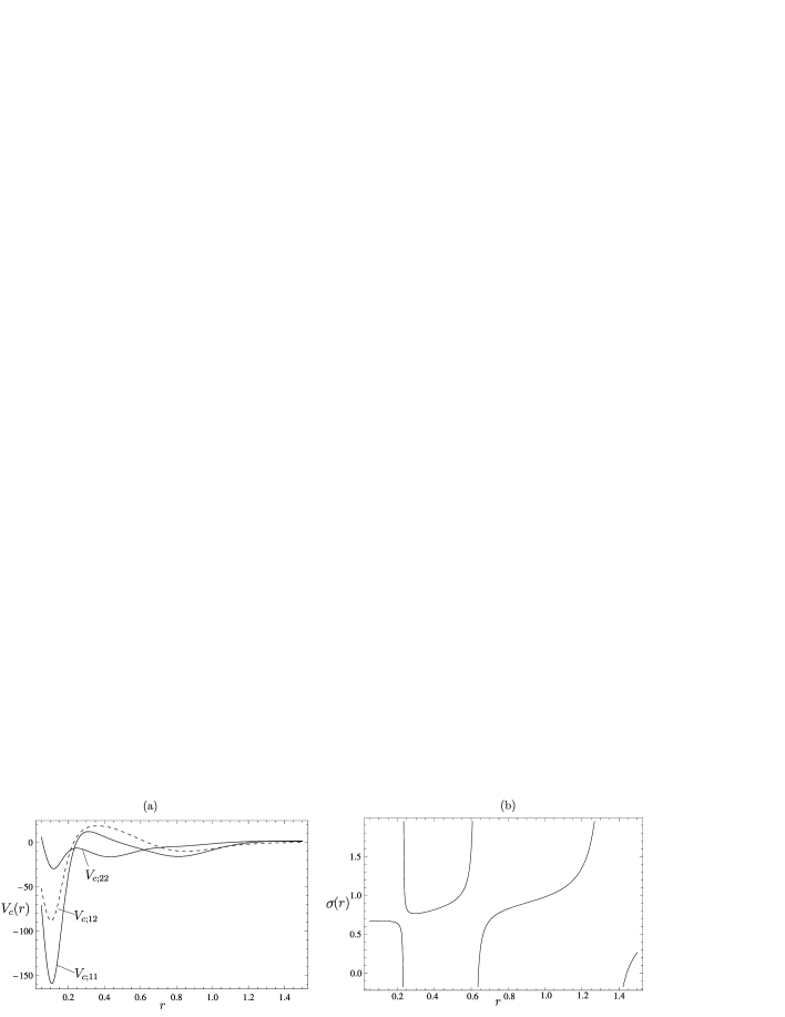
Figure 1: (a) Exactly solvable potential $\bar{V}_{c}=V_{c}$ obtained from two uncoupled potentials (63) ($\beta_{1}=-2\,,\beta_{2}=-1.5\,,\kappa_{0}=1\,,\kappa_{1}=2.5\,,\kappa_{2}=3.5$) by the coupling transformation with parameters $q=0.5$, $\kappa=6$, $x=25$. (b) Ratio $\sigma(r)=V_{c;12}(r)/\left(V_{c;22}(r)-V_{c;11}(r)\right)$.

To show the restrictive character of the requirement for the $S$ matrix to be non-trivially coupled, we construct below a potential with non-trivially coupled potential and Jost matrices but a trivially coupled $S$-matrix. This possibility is based on the fact that in the single-channel case two different Jost functions may correspond to the same scattering matrix [16, 29]. In this case, the two Jost functions differ from each other by a real factor for real $k$’s (see (3)). Therefore if we apply our coupling transformation to the following uncoupled system

$$V_{d}(r)=\mbox{\rm diag}\left[V_{1}(r),V_{2}(r)\right],\ \ \ F_{d}(k)=\mbox{\rm diag}\left[F_{1}(k),F_{2}(k)\right],\ \ \ S_{d}(k)=S(k)I_{2}\,,$$ (69)

from (69), (11), (30) and (51) we can see that the transformed potential and Jost matrices cannot be diagonalized by a constant rotation whereas the scattering matrix becomes diagonal after the same $k$-independent rotation which diagonalizes $w_{c\infty}$.

An example in which we get a non-diagonal Jost matrix and a trivially coupled $S$-matrix after applying the coupling transformation follows from (69) where we choose

$$F_{d}(k) = \mbox{\rm diag}\left[\frac{i(k-i\kappa_{0})}{(k+i\kappa_{1})(k+i\kappa_{2})},\frac{-i}{(k+i\kappa_{0})(k+i\kappa_{1})(k+i\kappa_{2})}\right],$$ (70)

$$S_{d}(k) = \frac{(k+i\kappa_{0})(k+i\kappa_{1})(k+i\kappa_{2})}{(k-i\kappa_{0})(k-i\kappa_{1})(k-i\kappa_{2})}I_{2}\,.$$ (71)

Here $\kappa_{0}$, $\kappa_{1}$ and $\kappa_{2}$ are arbitrary real parameters. Matrix $\nu$ for the corresponding potential

$$V_{d}(r)=\mbox{\rm diag}\left[V(r,\beta<-1),V(r,\beta=-1)\right]\,,$$ (72)

is $\nu=\mbox{\rm diag}(1,3)$ meaning that $\nu-1>0$ and we can apply the coupling transformation. Here the non-trivially coupled transformed Jost matrix (30) with $F_{d}$ as given in (70) leads to the following trivially coupled $S$-matrix

$$S_{c}(k)=(ikI_{2}-w_{c\infty})^{2}\frac{(k+i\kappa_{0})(k+i\kappa_{1})(k+i\kappa_{2})}{(k-i\kappa_{0})(k-i\kappa_{1})(k-i\kappa_{2})(k^{2}+\kappa^{2})}\,.$$ (73)

The corresponding phase shifts are given by (67) where $\delta_{c;2}\rightarrow\delta_{c;2}-\pi$ and the mixing angle is given by (66).

6.2 Coupled $s-s$ partial waves

Using our general scheme described in section 5, we can study the behaviour of the phase shifts for the $s-s$ coupled potential. Since the angular momenta in both channels coincide, we have here the case (iii) discussed above. Parameter $q$ is not fixed from the long-range behaviour of the potential and the mixing angle is given by (58). The analysis of this expression is based on the low-energy behaviour of the phase shifts $\delta_{d;1,2}$ before the coupling transformation

$$e^{2i\delta_{d;1,2}}=1-2ia_{1,2}k+{\rm o}(k)\,,$$ (74)

where $a_{1}$ and $a_{2}$ are the scattering lengths for each channel. Combining (58) and (74) we get

$$\tan 2\epsilon(k\rightarrow 0)=-\frac{2(1+(a_{1}-a_{2})\kappa\cos\alpha)\sin\alpha}{2\cos\alpha+(a_{1}-a_{2})\kappa\cos 2\alpha}+{\rm o}(k)\,.$$ (75)

The expansion of the eigenvalues of the transformed scattering matrix at low energies reads

$$e^{2i\delta_{c;1,2}}=1-ik\left[(a_{1}+a_{2})\pm\sqrt{(a_{2}-a_{1})^{2}+4\left(1/\kappa-(a_{2}-a_{1})\cos\alpha\right)/\kappa}\right]+{\rm o}(k)\,.$$ (76)

An important result from the point of view of inverse scattering corresponds to a coupling vanishing at low energies, i.e. when $\epsilon(0)=0$. This leads to an additional link between the parameters,

$$\cos\alpha=\frac{1}{(a_{2}-a_{1})\kappa}\,,$$ (77)

where we have used (75) and (5). Hence (76) simplifies into

$$e^{2i\delta_{c;1,2}}=1-2ia_{2,1}k+{\rm o}(k)\,.$$ (78)

In this case, the scattering lengths for the transformed potential coincide with the initial scattering lengths $a_{1}$ and $a_{2}$. This property allows us to fit low energy scattering data for uncoupled channels thus simplifying essentially the inverse problem. Let us illustrate this property in a schematic example.

We start from the zero potential with a transformation which introduces poles at the origin, $\nu=\mbox{\rm diag}(0,0)\rightarrow\nu=\mbox{\rm diag}(1,1)$. In each channel we realize the usual (i.e. $1$-channel) SUSY transformation with transformation functions $\sinh(\kappa_{1}r)$ and $\sinh(\kappa_{2}r)$. This leads to the uncoupled superpotential

$$w_{d}(r)=\mbox{\rm diag}\left[\kappa_{1}\coth(\kappa_{1}r),\kappa_{2}\coth(\kappa_{2}r)\right]$$ (79)

and the potential (see (11))

$$V_{d}(r)=2\mbox{\rm diag}\left[\kappa_{1}^{2}\mbox{\rm cosech}^{2}(\kappa_{1}r),\kappa_{2}^{2}\mbox{\rm cosech}^{2}(\kappa_{2}r)\right]\,,$$ (80)

with the Jost solution

$$f_{d}(k,r)=e^{ikr}\left(\begin{array}[]{cc}k+i\kappa_{1}\coth(\kappa_{1}r)&0\\ 0&k+i\kappa_{2}\coth(\kappa_{2}r)\end{array}\right)\left(\begin{array}[]{cc}k+i\kappa_{1}&0\\ 0&k+i\kappa_{2}\end{array}\right)^{-1}$$ (81)

and the Jost matrix

$$F_{d}(k)=(w_{d\infty}-ikI_{2})^{-1}\,,\quad w_{d\infty}=\lim_{r\to\infty}w_{d}(r)={\rm diag}\left(\kappa_{1},\kappa_{2}\right).$$ (82)

As coupling transformation we choose transformation function (15) with matrices $C$ and $D$ given by (37). The explicit expression for $u_{c}(r)$ coincides with (39) where

$$f_{d;1}(i\kappa,r)=\frac{\kappa+\kappa_{1}\coth(\kappa_{1}r)}{\kappa+\kappa_{1}}\,e^{-\kappa r}\,,\qquad f_{d;2}(i\kappa,r)=\frac{\kappa+\kappa_{2}\coth(\kappa_{2}r)}{\kappa+\kappa_{2}}\,e^{-\kappa r}\,.$$ (83)

The parameter $x$ from (37) should be chosen in order to avoid any singularity in the transformed potential. As can easily be seen from the analysis of ${\rm det\,}u_{c}$, it is sufficient to choose $x$ large enough. The asymptotic behaviour of the superpotential is given by (40) or (41).

The Jost matrix $F_{c}(k)$ may be found from (30). Its explicit expression is rather involved and we omit it. More important is its determinant (32), the expression of which is extremely simple,

$${\rm det\,}\,F_{c}(k)=\frac{k^{2}+\kappa^{2}}{(k+i\kappa_{1})(k+i\kappa_{2})}\,.$$ (84)

From here we find the location of the bound state at $k_{b}=i\kappa$ and the virtual state at $k_{v}=-i\kappa$.

The chain of two SUSY transformations with parameters $\kappa_{1,2}=a_{1,2}^{-1}$ and $\kappa,q,x$ described above leads to the mixing angle (75). The corresponding potential ($q=0.4$) is shown in figure 2. The factorization constant $\kappa$ is fixed from (77). As a result, the mixing angle takes the form

$$\tan 2\epsilon(k)=-\frac{2k^{2}\kappa_{1}\kappa_{2}\tan\alpha}{\kappa_{1}^{2}\kappa_{2}^{2}\sec^{2}\alpha+k^{2}(\kappa_{1}^{2}+\kappa_{2}^{2})}\,.$$ (85)

Parameters $\kappa_{1}$ and $\kappa_{2}$ are related with $1$-channel transformations and allow us to fit the scattering lengths. The mixing angle $\epsilon(k)$ depends on parameter $\alpha$, which allows one to fit its experimental behaviour at low energies. The mixing angle at large energies tends to a constant value, $\tan 2\epsilon(k\to\infty)=-2\kappa_{1}\kappa_{2}\tan\alpha/(\kappa_{1}^{2}+\kappa_{2}^{2})$ which can also be fitted using corresponding experimental data (if available). Figure 3 shows the phase shifts and mixing angle for two coupled $s-s$ potentials.

Figure 2: Exactly solvable $s-s$ potential $\bar{V}_{c}=V_{c}$ with parameters $\kappa_{1}=1.5$, $\kappa_{2}=1$, $q=0.4$, $\kappa=4.14286$, $x=15$.

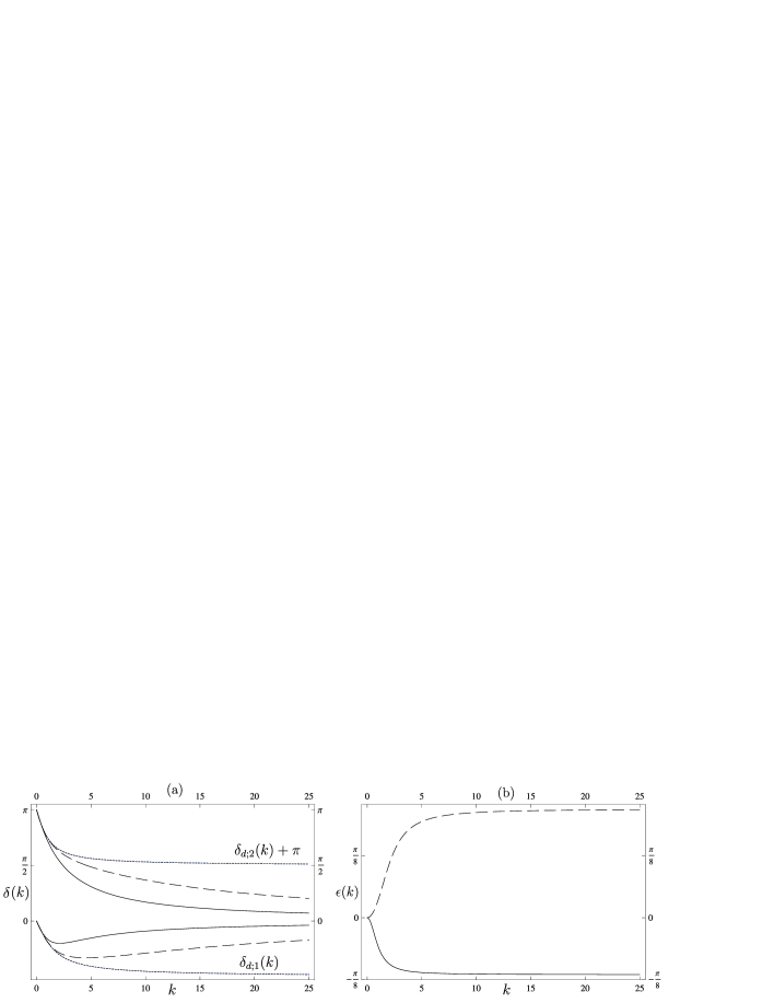
Figure 3: The scattering matrix for the coupled $s-s$ potential. (a) The eigenphases are shown as dotted lines for $V_{d}$ and as dashed and solid lines for $V_{c}$. The parameters are: solid lines - $\kappa_{1}=1.5$, $\kappa_{2}=1$, $q=0.4$, $\kappa=4.14286$, $x=15$, dashed lines - $\kappa_{1}=1.5$, $\kappa_{2}=1$, $q=1.2$, $\kappa=13.6667$, $x=15$. (b) Mixing angle $\epsilon$.

The phase shifts of the diagonal potential $V_{d}$ are shown as dotted lines in figure 3(a). The phase shifts of the transformed potential $V_{c}$ are shown as dashed ($q=0.4$) and solid ($q=1.2$) lines respectively. One can see that the slopes of these curves coincide at the origin. The mixing angles of the transformed potential are plotted in figure 3(b).

According to (84) this potential has one bound state at the factorization energy $E_{g}=-\kappa^{2}$. Note that the normalization constant of the bound state wave function is determined by parameter $q$ as follows from (33).

6.3 Coupled $s-p$ partial waves

Figure 4: Exactly solvable $s-p$ potential $\bar{V}_{c}=V_{c}-\tilde{l}(\tilde{l}+1)r^{-2}$ with parameters $\kappa_{0}=1.5$, $\kappa_{1}=1.75$, $\kappa=3.53$, $q=1$, $x=1$.

In this section we consider the simplest $s-p$ coupled potential. This potential is characterized by $\tilde{l}=\tilde{\nu}=\mbox{\rm diag}(1,0)$. The coupling transformation acts as follows:

$$l=\mbox{\rm diag}(l_{1},l_{2})\rightarrow\tilde{l}=\mbox{\rm diag}(l_{2},l_{1})\,,\qquad\nu=\mbox{\rm diag}(\nu_{1},\nu_{2})\rightarrow\tilde{\nu}=\mbox{\rm diag}(\nu_{1}-1,\nu_{2}-1)\,.$$ (86)

Therefore the initial diagonal potential should have $l=\mbox{\rm diag}(0,1)$, $\nu=(2,1)$. These properties are satisfied for the initial potential of the form

$$V_{d}(r)=\mbox{\rm diag}\left[-2\frac{d^{2}}{dr^{2}}\ln W[\sinh\left(\kappa_{0}r\right),\sinh\left(\kappa_{1}r\right)],2r^{-2}\right],$$ (87)

where the potential in the $s$-channel is obtained from the zero potential after two consecutive SUSY transformations with $\kappa_{0}$ and $\kappa_{1}$ as factorization constants. The potential in the $p$-channel is just the centrifugal term. The Jost solution in the $s$-channel is expressed in terms of the Wronskian of factorization solutions $\sinh(\kappa_{j}r)$, $j=0,1$,

$$f_{d}(k,r)=\mbox{\rm diag}\left[\frac{W\left[\sinh\left(\kappa_{0}r\right),\sinh\left(\kappa_{1}r\right),e^{ikr}\right]}{(k+i\kappa_{0})(k+i\kappa_{1})W\left[\sinh\left(\kappa_{0}r\right),\sinh\left(\kappa_{1}r\right)\right]},\frac{(i+kr){\rm e}^{ikr}}{kr}\right].$$ (88)

The uncoupled Jost matrix reads

$$F_{d}(k)=\mbox{\rm diag}\left[-\left[(k+i\kappa_{0})(k+i\kappa_{1})\right]^{-1},ik^{-1}\right].$$ (89)

The next step is to apply the coupling transformation with the transformation function (15) where the Jost solution is replaced by (88). An example of potential curves is shown in figure 4. The Jost matrix (89) is transformed according to (30) and the scattering matrix is given by (51).

Since the transformed eigenphase shifts coincide with the initial phase shifts, we may fit the phase shifts for the $s$ and $p$ waves separately before the coupling transformation. In our example the phase shifts read

$$\delta_{c;1}(k)=0\,,\qquad\delta_{c;2}(k)=\pi-\arctan\frac{k}{\kappa_{0}}-\arctan\frac{k}{\kappa_{1}}\,.$$ (90)

Parameters $\kappa_{0}$ and $\kappa_{1}$ allow one to fit the $s$-channel phase shifts. Parameter $\kappa$ may be used to fit the slope of the mixing angle (59) at zero energy. If necessary, one may use arbitrary chains of 1-channel transformations to get the best fit of the phase shifts.

6.4 Coupled $s-d$ partial waves

The simplest $s-d$ coupled potential is characterized by $\tilde{l}=\tilde{\nu}=\mbox{\rm diag}(2,0)$. Therefore the initial diagonal potential should have $l=\mbox{\rm diag}(0,2)$ and $\nu=(3,1)$. Moreover, as we established in section 5, $\delta_{d;2}(0)-\delta_{d;1}(0)=(n+1/2)\pi$ which for $n=0$ leads to the following initial phase shifts $\delta_{d;2}(0)=\pi/2$ and $\delta_{d;1}(0)=0$.

We start with the initial $s$-wave potential

$$V_{0}(r)=\frac{-2\kappa_{0}^{2}}{\cosh^{2}(\kappa_{0}r)}$$ (91)

having a zero energy virtual state [3] which follows from its Jost function

$$F_{0}(k)=\frac{k}{k+i\kappa_{0}}\,.$$ (92)

Note that this potential and the solutions of the corresponding Schrödinger equation may be obtained by a SUSY transformation. This is a regular potential. To be able to apply the coupling transformation, we increase its singularity at the origin using three SUSY transformations with the transformation functions

$$u(\kappa_{i},r)=\kappa_{i}\sinh(\kappa_{i}r)+\kappa_{0}\cosh(\kappa_{i}r)\tanh(\kappa_{0}r)\,,\qquad i=1,2,3\,.$$ (93)

The potential and the Jost function in the $s$-channel after these transformations read

$$V_{d;1}(r)=\frac{-2\kappa_{0}^{2}}{\cosh^{2}(\kappa_{0}r)}-2\left(\ln W\left[u(\kappa_{1},r),u(\kappa_{2},r),u(\kappa_{3},r)\right]\right)^{\prime\prime},$$ (94)

$$F_{d;1}(k)=\frac{-ik}{(k+i\kappa_{0})(k+i\kappa_{1})(k+i\kappa_{2})(k+i\kappa_{3})}\,.$$ (95)

The potential in the $d$-channel

$$V_{d;2}(r) = \frac{6}{r^{2}}-2\ln v^{\prime\prime}(\kappa_{4},r)=\frac{6(3+6\kappa_{4}x+6\kappa_{4}^{2}r^{2}+4\kappa_{4}^{3}r^{3}+\kappa_{4}^{4}r^{4})}{r^{2}(3+3\kappa_{4}r+\kappa_{4}^{2}r^{2})^{2}}\,,$$ (96)

$$v(\kappa_{4},r) = {\rm e}^{-\kappa_{4}r}\left(1+{3}{\kappa_{4}r}+\frac{3}{(\kappa_{4}r)^{2}}\right),$$ (97)

is obtained from the centrifugal term $6/r^{2}$ by the SUSY transformation with $v(r,\kappa_{4})$ as the transformation function, which decreases the singularity of the potential at the origin.

Figure 5: Exactly solvable $s-d$ potential $\bar{V}_{c}=V_{c}-\tilde{l}(\tilde{l}+1)r^{-2}$ with parameters $\kappa_{0}=1$, $\kappa_{1}=1.5$, $\kappa_{2}=1.75$, $\kappa_{3}=2$, $\kappa_{4}=3$ $q=1$, $x=15$, $\kappa=5.53$.

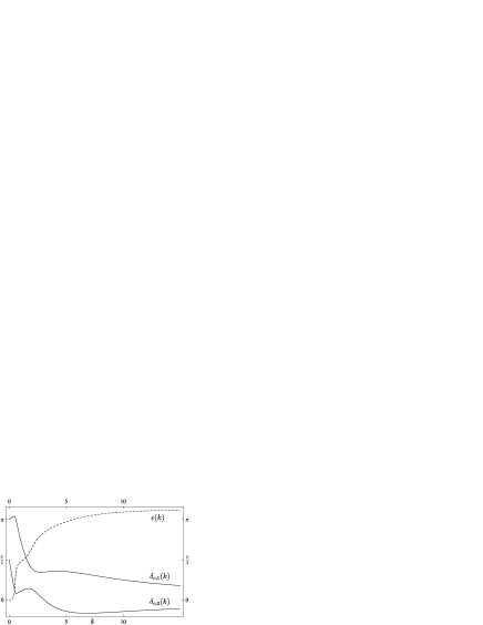
Figure 6: The scattering matrix for the coupled $s-d$ potential. The phase shifts $\delta_{c;1}(k)$ and $\delta_{c;2}(k)$ are plotted by solid lines. The mixing angle $\epsilon(k)$ is plotted by the dashed line. The corresponding parameters are $\kappa_{0}=1$, $\kappa_{1}=1.5$, $\kappa_{2}=1.75$, $\kappa_{3}=2$, $\kappa_{4}=3$ $q=1$, $x=15$, $\kappa=5.53$.

The Jost solution in the $s$-channel is expressed in terms of the Wronskian of factorization solutions (93)

$$f_{d;1}(k,r) = \frac{W\left[u(\kappa_{1},r),u(\kappa_{2},r),u(\kappa_{3},r),f_{0}(k,r)\right]}{(k+i\kappa_{1})(k+i\kappa_{2})(k+i\kappa_{3})W\left[u(\kappa_{1},r),u(\kappa_{2},r),u(\kappa_{3},r)\right]}\,,$$ (98)

$$f_{0}(k,r) = {\rm e}^{ikr}\frac{k+i\kappa_{0}\tanh(\kappa_{0}r)}{k+i\kappa_{0}}\,.$$ (99)

The Jost solution in the $d$-channel is

$$f_{d;2}(k,r)=i\frac{W\left[v(\kappa_{4},r),h_{2}(kr)\right]}{(k-i\kappa_{4})v(\kappa_{4},r)}\,,\qquad h_{2}(kr)={\rm e}^{ikr}\left(1+{3i}{\kappa_{4}r}-\frac{3}{(\kappa_{4}r)^{2}}\right).$$ (100)

The uncoupled Jost matrix reads

$$F_{d}(k)=\mbox{\rm diag}\left[\frac{-ik}{(k+i\kappa_{0})(k+i\kappa_{1})(k+i\kappa_{2})(k+i\kappa_{3})},\frac{ik-\kappa_{4}}{k^{2}}\right],$$ (101)

which produces the eigenphase shifts

$$\delta_{d;1}(k)=\frac{\pi}{2}-\sum\limits_{j=0}^{3}\arctan\frac{k}{\kappa_{j}}\,,\qquad\delta_{d;2}(k)=\arctan\frac{k}{\kappa_{4}}\,.$$ (102)

Next we apply the coupling transformation with the transformation function (15) where the Jost solution $f_{d}=\mbox{\rm diag}(f_{d;1},f_{d;2})$ is combined from (98) and (100). An example of potential curves thus obtained is shown in figure 5. The Jost matrix (101) is transformed according to (30) and the scattering matrix is given by (51).

The corresponding phase shifts and mixing angle are plotted in figure 6. The mixing parameter $\epsilon(k)$ is determined by (60) which, in the current case, reduces to

$$\tan 2\epsilon(k)=\frac{2\kappa k}{(k^{2}+\kappa^{2})}\tan\left(\sum\limits_{j=0}^{4}\arctan\frac{k}{\kappa_{j}}\right).$$ (103)

We were not able to find simple expressions for the eigenphase shifts in this case. One can see that the mixing parameter satisfies the effective range expansion (5) (see (103) and figure 6). Unfortunately, this is not the case for the phase shifts (see figure 6).

7 Conclusion

In the present paper, a careful analysis of SUSY transformations between uncoupled potentials with equal thresholds but arbitrary partial waves in $N$ channels and coupled ones is given. In particular, we formulated conditions imposed on the transformation function to get a nontrivially coupled scattering matrix. A family of iso-phase potentials generated by a coupling SUSY transformation has been obtained. This family is parameterized by a real symmetric $M\times M$, $0<M<N$, non-singular matrix $X_{0}$. The analysis of the zeros of the Jost-matrix determinant for these potentials showed that the SUSY transformation creates a new $M$ fold degenerate bound state energy $E_{b}=-\kappa^{2}$ and an $N-M$ fold degenerate virtual state energy $E_{v}=-\kappa^{2}$.

In the most important practical case, the two-channel case, we analyzed the behaviour of the superpotential and potential at large distances in details. We have found an unusual effect, i.e. a modification of the long-range behaviour of the potential under a coupling SUSY transformation which consists in the exchange of attribution of the partial waves between the channels. Moreover, we analyzed in details the transformed scattering matrix, phase shifts and mixing angle. The analysis of the phase shifts and mixing angle demonstrated how scattering properties change after a SUSY transformation.

As an illustration of our approach, several simple examples have been presented. First, to emphasize the difference between couplings in the potential, Jost and scattering matrices, we presented examples of a trivially coupled scattering matrix corresponding to non trivially coupled potential and Jost matrices. These examples answer the general questions raised in the introduction: situations may exist where a non trivially coupled potential leads to a trivially coupled $S$-matrix, with either a trivially or non trivially coupled Jost matrix. Thus, the requirement that an $S$-matrix is non trivially coupled is more restrictive than the similar requirement for a potential matrix. Moreover, even the requirement that the Jost matrix is non trivially coupled is less restrictive than the corresponding requirement for the $S$-matrix.

Afterwards, a non trivial coupling was introduced in the $s-s$, $s-p$ and $s-d$ channels. In both $s-s$ and $s-p$ examples, we have shown how to fit the low-energy behaviour of the phase shifts and mixing angle using parameters of the transformation. We note that the $s-p$ example contains all essential ingredients of a convenient inversion scheme since the $s-p$ coupling transformation conserves the initial phase shifts, which allows separating the inversion of phase shifts from that of coupling parameters. In the $s-d$ case, to satisfy the effective range expansion for the mixing parameter, we used an initial potential with a zero energy virtual state. Nevertheless, the obtained phase shifts of the coupled $s-d$ potential do not satisfy the correct effective range expansion. Moreover, the presence of the zero energy virtual state strongly restricts possible applications of our method to the inversion in this case. We believe that a chain of two coupling transformations may allow avoiding this inconvenience.

References

References

- [1] Novikov S P, Manakov S V , Pitaevskii L P and Zakharov V E 1984 Theory of Solitons: The Inverse Scattering Method (Monographs in Contemporary Mathematics) (New York: Springer)
- [2] Ablowitz M A and Clarkson P A 1992 Solitons, Nonlinear Evolution Equations and Inverse Scattering (Cambridge: Cambridge University Press)
- [3] Newton R G 1982 Scattering Theory of Waves and Particles (New York: Springer)
- [4] Taylor J R 1972 Scattering Theory: The Quantum Theory on Nonrelativistic Collisions (New York: Wiley)
- [5] Levitan B M 1984 Inverse Sturm-Liouville Problems (Moscow: Nauka)
- [6] Chadan K and Sabatier P C 1989 Inverse Problems in Quantum Scattering Theory, 2nd edn. (New York: Springer).
- [7] Matveev V and Salle M 1991 Darboux Transformations and Solitons (New York: Springer)
- [8] Cooper F, Khare A and Sukhatme U 2001 Supersymmetry in Quantum Mechanics (Singapore: World Scientific)
- [9] Bagchi B K 2001 Supersymmetry in Quantum and Classical Mechanics (New York: Chapman and Hall)
- [10] Baye D and Sparenberg J-M 2004 Inverse scattering with supersymmetric quantum mechanics J. Phys. A: Math. Gen. 37 10223-49
- [11] Amado R D, Cannata F and Dedonder J-P 1988 Formal scattering theory approach to S-matrix relations in supersymmetric quantum mechanics Phys. Rev. Lett. 61 2901-4
- [12] Amado R D, Cannata F and Dedonder J-P 1988 Coupled-channel supersymmetric quantum mechanics Phys. Rev. A 38 3797-800
- [13] Amado R D, Cannata F and Dedonder J-P 1990 Supersymmetric quantum mechanics coupled channels scattering relations Int. J. Mod. Phys. A 5 3401-15
- [14] Cannata F and Ioffe M V 1992 Solvable coupled channel problems from supersymmetric quantum mechanics Phys. Lett. B 278 399-402
- [15] Cannata F and Ioffe M V 1993 Coupled channel scattering and separation of coupled differential equations by generalized Darboux transformations J. Phys. A: Math. Gen 26 L89-92
- [16] Sparenberg J-M and Baye D 1996 Supersymmetry between deep and shallow optical potentials for 16O + 16O scattering Phys. Rev. C 54 1309-21
- [17] Sparenberg J-M and Baye D 1997 Supersymmetry between phase-equivalent coupled-channel potentials Phys. Rev. Lett. 79 3802-5
- [18] Leeb H, Sofianos S A, Sparenberg J-M and Baye D 2000 Supersymmetric transformations in coupled-channel systems Phys. Rev. C 62 064003
- [19] Sparenberg J-M, Samsonov B F, Foucart F and Baye D 2006 Multichannel coupling with supersymmetric quantum mechanics and exactly-solvable model for Feshbach resonance J. Phys. A: Math. Gen. 39 L639-45
- [20] Samsonov B F, Sparenberg J-M and Baye D 2007 Supersymmetric transformations for coupled channels with threshold differences J. Phys. A: Math. Theor. 40 4225-40
- [21] Pupasov A M, Samsonov B F and Sparenberg J-M 2008 Spectral properties of non-conservative multichannel SUSY partners of the zero potential J. Phys. A: Math. Theor. 41 175209
- [22] Sparenberg J-M, Pupasov A M, Samsonov B F and Baye D 2008 Exactly-solvable coupled-channel models from supersymmetric quantum mechanics Mod. Phys. Lett. B 22 2277-86
- [23] Cox J R 1964 Many-channel Bargmann potentials J. Math. Phys. 5 1065-9
- [24] Pupasov A M, Samsonov B F and Sparenberg J-M 2008 Exactly-solvable coupled-channel potential models of atom-atom magnetic Feshbach resonances from supersymmetric quantum mechanics Phys. Rev. A 77 012724 (Preprint quant-ph/0709.0343)
- [25] Newton R G and Fulton T 1982 Phenomenological neutron-proton potentials Phys. Rev. 107 1103-11
- [26] Samsonov B F and Stancu F 2003 Phase shifts effective range expansion from supersymmetric quantum mechanics Phys. Rev. C 67 054005
- [27] Bagrov V G and Samsonov B F 1995 Darboux transformation, factorization and supersymmetry in one-dimensional quantum mechanics Theor. Math. Phys. 104 1051-60
- [28] Baye D 1987 Supersymmetry between deep and shallow nucleus-nucleus potentials Phys. Rev. Lett. 58 2738-41
- [29] Samsonov B F and Stancu F 2002 Phase equivalent chains of Darboux transformations in scattering theory Phys. Rev. D 66 034001
- [30] Erdélyi A 1953 Higher Transcendental Functions 2 (New York: McGraw-Hill)
- [31] Fulton N and Newton R G 1956 Explicit non-central potentials and wave functions for given -matrices Il Nuovo Cimento 3 677-717
- [32] Delves L M 1958 Effective range expansion of the scattering matrix Nuclear physics 8 358-73
- [33] Bargmann V 1949 Remarks on the determination of a central field of force from the elastic scattering phase shifts Phys. Rev. 75 301-3