Multipole Representation of the Fermi Operator with Application to the Electronic Structure Analysis of Metallic Systems

Abstract

We propose a multipole representation of the Fermi-Dirac function and the Fermi operator, and use this representation to develop algorithms for electronic structure analysis of metallic systems. The new algorithm is quite simple and efficient. Its computational cost scales logarithmically with $\beta\Delta\epsilon$ where $\beta$ is the inverse temperature, and $\Delta\epsilon$ is the width of the spectrum of the discretized Hamiltonian matrix.

I Introduction

The Fermi operator, i.e. the Fermi-Dirac function of the system Hamiltonian, is a fundamental quantity in the quantum mechanics of many-electron systems and is ubiquitous in condensed matter physics. In the last decade the development of accurate and numerically efficient representations of the Fermi operator has attracted lot of attention in the quest for linear scaling electronic structure methods based on effective one-electron Hamiltonians. These approaches have numerical cost that scales linearly with $N$, the number of electrons, and thus hold the promise of making quantum mechanical calculations of large systems feasible. Achieving linear scaling in realistic calculations is very challenging. Formulations based on the Fermi operator are appealing because this operator gives directly the single particle density matrix without the need for Hamiltonian diagonalization. At finite temperature the density matrix can be expanded in terms of finite powers of the Hamiltonian, requiring computations that scale linearly with $N$ owing to the sparse character of the Hamiltonian matrix. These properties of the Fermi operator are valid not only for insulators but also for metals, making formulations based on the Fermi operator particularly attractive.

Electronic structure algorithms using a Fermi operator expansion (FOE) were introduced by Baroni and Giannozzi Baroni and Giannozzi (1992) and Goedecker and co-workers Goedecker and Colombo (1994); Goedecker and Teter (1995) (see also the review article Goedecker (1999)). These authors proposed polynomial and rational approximations of the Fermi operator. Major improvements were made recently in a series of publications by Parrinello and co-authors Krajewski and Parrinello (2005); Krajewski and Parrinello (2006a, b); Krajewski and Parrinello (2007); Ceriotti et al. (2008a, b), in which a new form of Fermi operator expansion was introduced based on the grand canonical formalism.

From the viewpoint of efficiency, a major concern is the cost of the representations of the Fermi operator as a function of $\beta\Delta\epsilon$ where $\beta$ is the inverse temperature and $\Delta\epsilon$ is the spectral width of the Hamiltonian matrix. The cost of the original FOE proposed by Goedecker et al scales as $\beta\Delta\epsilon$. The fast polynomial summation technique introduced by Head-Gordon et alLiang et al. (2003, 2004) reduces the cost to $(\beta\Delta\epsilon)^{1/2}$. The cost of the hybrid algorithm proposed by Parrinello et al in a recent preprint Ceriotti et al. (2008b) scales as $(\beta\Delta\epsilon)^{1/3}$.

The main purpose of this paper is to present a strategy that reduces the cost to logarithmic scaling $(\ln\beta\Delta\epsilon)\cdot(\ln\ln\beta\Delta\epsilon)$, thus greatly improving the efficiency and accuracy of numerical FOEs. Our approach is based on the exact pole expansion of the Fermi-Dirac function which underlies the Matsubara formalism of finite temperature Green’s functions in many-body physics Mahan (2000). It is natural to consider a multipole representation of this expansion to achieve better efficiency, as was done in the fast multipole method Greengard and Rokhlin (1987). Indeed, as we will show below, the multipole expansion that we propose does achieve logarithmic scaling. We believe that this representation will be quite useful both as a theoretical tool and as a starting point for computations. As an application of the new formalism, we present an algorithm for electronic structure calculation that has the potential to become an efficient linear scaling algorithm for metallic systems.

The remaining of the paper is organized as follows. In the next section, we introduce the multipole representation of Fermi operator. In Section III, we present the FOE algorithm based on the multipole representation and analyze its computational cost. Three examples illustrating the algorithm are discussed in Section IV. We conclude the paper with some remarks on future directions.

II Multipole representation for the Fermi operator

Given the effective one-particle Hamiltonian $\boldsymbol{\mathrm{H}}$, the inverse temperature $\beta=1/k_{\mathrm{B}}T$ and the chemical potential $\mu$, the finite temperature single-particle density matrix of the system is given by the Fermi operator

$$\boldsymbol{\mathrm{\rho}}=\frac{2}{1+\exp(\beta(\boldsymbol{\mathrm{H}}-\mu))}=1-\tanh\Bigl{(}\frac{\beta}{2}(\boldsymbol{\mathrm{H}}-\mu)\Bigr{)},$$ (1)

where $\tanh$ is the hyperbolic tangent function. The Matsubara representation of the Fermi-Dirac function is given by

$$\boldsymbol{\mathrm{\rho}}=1-4\mathrm{Re}~{}\sum_{l=1}^{\infty}\frac{1}{\beta(\boldsymbol{\mathrm{H}}-\mu)-(2l-1)\pi i}.$$ (2)

This representation originates from the pole expansion (see, for example, Jeffreys and Jeffreys (1956); Ahlfors (1978)) of the meromorphic function $\tanh$

$$\tanh z=\sum_{l=-\infty}^{\infty}\frac{1}{z-\frac{2l-1}{2}\pi i}.$$ (3)

In particular, for $x$ real (which is the case when $\boldsymbol{\mathrm{H}}$ is self-adjoint), we have

$$\tanh x=4\mathrm{Re}~{}\sum_{l=1}^{\infty}\frac{1}{2x-(2l-1)\pi i}.$$ (4)

To make the paper self-contained, we provide in Appendix A a simple derivation of this representation. It should be emphasized that (2) is exact. We notice that the expansion (2) can also be understood as the $P\to\infty$ limit of an exact Fermi operator expansion proposed by Parrinello and co-authors in Krajewski and Parrinello (2005); Krajewski and Parrinello (2006a, b); Krajewski and Parrinello (2007); Ceriotti et al. (2008a, b).

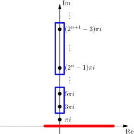
Figure 1: (color online) Illustration of the pole decomposition (13). From $2^{n}$ to $2^{n+1}-1$ poles are grouped together as shown in the figure. The spectrum is indicated by the red line on the real axis.

The summation in (2) can be seen as a summation of residues contributed from the poles $\{(2l-1)\pi i\}$, with $l$ a positive integer, on the imaginary axis. This suggests to look for a multipole expansion of the contributions from the poles, as done in the fast multipole method (FMM) Greengard and Rokhlin (1987). To do so, we use a dyadic decomposition of the poles, in which the $n$-th group contains terms from $l=2^{n-1}$ to $l=2^{n}-1$, for a total of $2^{n-1}$ terms (see Figure 1 for illustration). We decompose the summation in Eq.(2) accordingly, denoting $x=\beta(\boldsymbol{\mathrm{H}}-\mu)$ for simplicity

$$\sum_{l=1}^{\infty}\frac{1}{x-(2l-1)\pi i}=\sum_{n=1}^{\infty}\sum_{l=2^{n-1}}^{2^{n}-1}\frac{1}{x-(2l-1)\pi i}=\sum_{n=1}^{\infty}S_{n}.$$ (5)

The basic idea is to combine the simple poles into a set of multipoles at $l=l_{n}$, where $l_{n}$ is taken as the midpoint of the interval $[2^{n-1},2^{n}-1]$

$$l_{n}=\frac{3\cdot 2^{n-1}-1}{2}.$$ (6)

Then the $S_{n}$ term in the above equation can be written as

$$S_{n} =\sum_{l=2^{n-1}}^{2^{n}-1}\frac{1}{x-(2l_{n}-1)\pi i-2(l-l_{n})\pi i}$$ (7)

$$=\sum_{l=2^{n-1}}^{2^{n}-1}\frac{1}{x-(2l_{n}-1)\pi i}\sum_{\nu=0}^{\infty}\Bigl{(}\frac{2(l-l_{n})\pi i}{x-(2l_{n}-1)\pi i}\Bigr{)}^{\nu}$$

$$=\sum_{l=2^{n-1}}^{2^{n}-1}\frac{1}{x-(2l_{n}-1)\pi i}\sum_{\nu=0}^{P-1}\Bigl{(}\frac{2(l-l_{n})\pi i}{x-(2l_{n}-1)\pi i}\Bigr{)}^{\nu}$$

$$\qquad\qquad+\sum_{l=2^{n-1}}^{2^{n}-1}\frac{1}{x-(2l-1)\pi i}\Bigl{(}\frac{2(l-l_{n})\pi i}{x-(2l_{n}-1)\pi i}\Bigr{)}^{P}$$

In deriving Eq. (7) we used the result for the sum of a geometric series. Using the fact that $x$ is real, the second term in Eq. (7) can be bounded by

$$\sum_{l=2^{n-1}}^{2^{n}-1}\Bigl{\lvert}\frac{1}{x-(2l-1)\pi i}\Bigr{\rvert}\Bigl{\lvert}\frac{2(l-l_{n})\pi i}{x-(2l_{n}-1)\pi i}\Bigr{\rvert}^{P}\leq\sum_{l=2^{n-1}}^{2^{n}-1}\frac{1}{\lvert(2l-1)\pi\rvert}\Bigl{\lvert}\frac{2(l-l_{n})}{2l_{n}-1}\Bigr{\rvert}^{P}\leq\frac{1}{2\pi}\frac{1}{3^{P}}$$ (8)

Therefore, we can approximate the sum $S_{n}$ by the first $P$ terms, and the error decays exponentially with $P$:

$$\left\lvert S_{n}(x)-\sum_{l=2^{n-1}}^{2^{n}-1}\frac{1}{x-(2l_{n}-1)\pi i}\sum_{\nu=0}^{P-1}\Bigl{(}\frac{2(l-l_{n})\pi i}{x-(2l_{n}-1)\pi i}\Bigr{)}^{\nu}\right\rvert\leq\frac{1}{2\pi}\frac{1}{3^{P}},$$ (9)

uniformly in $x$. The above analysis is of course standard from the view point of the fast multipole method Greengard and Rokhlin (1987). The overall philosophy is also similar: given a preset error tolerance, one selects $P$, the number of terms to retain in $S_{n}$, according to Eq. (9).

Interestingly, the remainder of the sum in Eq. (2) from $l=m$ to $\infty$ has an explicit expression

$$\mathrm{Re}~{}\sum_{l=m}^{\infty}\dfrac{1}{2x-(2l-1)i\pi}=\frac{1}{2\pi}\mathrm{Im}~{}\psi\left(m-\frac{1}{2}+\frac{i}{\pi}x\right),$$ (10)

where $\psi$ is the digamma function $\psi(z)=\Gamma^{\prime}(z)/\Gamma(z)$. It is well known Jeffreys and Jeffreys (1956) that the digamma function has the following asymptotic expansion

$$\psi(z)\sim\ln(z)-\frac{1}{2z}-\frac{1}{12z^{2}}+\mathcal{O}\Bigl{(}\frac{1}{z^{4}}\Bigr{)},\quad\lvert\arg z\rvert\leq\pi\text{ and }\lvert z\rvert\to\infty.$$ (11)

Therefore,

$$\mathrm{Im}~{}\psi\left(m-\frac{1}{2}+\frac{i}{\pi}x\right) \sim\mathrm{Im}~{}\ln\left(m-\frac{1}{2}-\frac{i}{\pi}x\right)+\mathcal{O}\Bigl{(}\frac{1}{m^{2}}\Bigr{)}$$ (12)

$$=\arctan\left(\frac{2x}{(2m-1)\pi}\right)+\mathcal{O}\Bigl{(}\frac{1}{m^{2}}\Bigr{)},\quad m\to\infty.$$

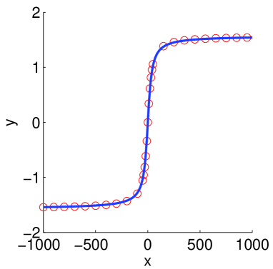
Figure 2: (color online) The function $\mathrm{Im}~{}\psi\left(m-\frac{1}{2}+\frac{i}{\pi}x\right)$(red circle), i.e. the remainder of the pole expansion in Eq. (13) is compared with the function $\arctan\left(\frac{2x}{(2m-1)\pi}\right)$ (blue solid line) for $m=10$

Figure 2 shows that the asymptotic approximation (12) is already rather accurate when $m=10$.

Eq. (12) also shows the effectiveness of the multipole representation from the viewpoint of traditional polynomial approximations. At zero temperature, the Fermi-Dirac function is a step function that cannot be accurately approximated by any finite order polynomial. At finite but low temperature, it is a continuous function with a very large derivative at $x=0$, i.e. when the energy equals the chemical potential $\mu$. The magnitude of this derivative becomes smaller and, correspondingly, the Fermi function becomes smoother as the temperature is raised. One can use the value of the derivative of the Fermi function at $x=0$ to measure the difficulty of an FOE. After eliminating the first $m$ terms in the expansion, Eq. (12) shows that asymptotically the derivative is multiplied by the factor $\frac{2}{(2m-1)\pi}$, which is equivalent to a rescaling of the temperature by the same factor. In particular, if we explicitly include the first $2^{N}$ terms in the multipole representation of the Fermi operator, we are left with a remainder which is well approximated by Eq. (12), so that, effectively, the difficulty is reduced by a factor $2^{N}$. As a matter of fact standard polynomials approximations, such as the Chebyshev expansion, can be used to efficiently represent the remainder in Eq. (10) even at very low temperature.

In summary, we arrive at the following multipole representation for the Fermi operator

$$\boldsymbol{\mathrm{\rho}}=1-4\mathrm{Re}~{}\sum_{n=1}^{N}\sum_{l=2^{n-1}}^{2^{n}-1}\frac{1}{\beta(\boldsymbol{\mathrm{H}}-\mu)-(2l_{n}-1)\pi i}\sum_{\nu=0}^{P-1}\Bigl{(}\frac{2(l-l_{n})\pi i}{\beta(\boldsymbol{\mathrm{H}}-\mu)-(2l_{n}-1)\pi i}\Bigr{)}^{\nu}\\ -\frac{2}{\pi}\mathrm{Im}~{}\psi\left(2^{N}-\frac{1}{2}+\frac{i}{2\pi}\beta(\boldsymbol{\mathrm{H}}-\mu)\right)+\mathcal{O}(N/3^{P}).$$ (13)

The multipole part is evaluated directly as discussed below, and the remainder is evaluated with the standard polynomial method.

III Numerical calculation and error analysis

To show the power of the multipole expansion, we discuss a possible algorithm to compute the Fermi operator in electronic structure calculations and present a detailed analysis of its cost in terms of $\beta\Delta\epsilon$. Given the Hamiltonian matrix $\boldsymbol{\mathrm{H}}$, it is straightforward to compute the density matrix $\boldsymbol{\mathrm{\rho}}$ from the multipole expansion if we can calculate the Green’s functions $\boldsymbol{\mathrm{B}}_{l_{n}}=\left[\beta(\boldsymbol{\mathrm{H}}-\mu)-(2l_{n}-1)\pi i\right]^{-1}$ for different $n$.

A possible way to calculate the inverse matrices is by the Newton-Schulz iteration. For any non-degenerate matrix $\boldsymbol{\mathrm{A}}$, the Newton-Schulz iteration computes the inverse $\boldsymbol{\mathrm{B}}=\boldsymbol{\mathrm{A}}^{-1}$ as

$$\boldsymbol{\mathrm{B}}_{k+1}=2\boldsymbol{\mathrm{B}}_{k}-\boldsymbol{\mathrm{B}}_{k}\boldsymbol{\mathrm{A}}\boldsymbol{\mathrm{B}}_{k}.$$ (14)

The iteration error is measured by the spectral radius, i.e. the eigenvalue of largest magnitude, of the matrix $\boldsymbol{\mathrm{I}}-\boldsymbol{\mathrm{B}}\boldsymbol{\mathrm{B}}_{k}$ where $\boldsymbol{\mathrm{I}}$ is the identity matrix. In the following we denote the spectral radius of the matrix $\boldsymbol{\mathrm{A}}$ by $\sigma(\boldsymbol{\mathrm{A}})$. Then the spectral radius at the $k$-th step of the Newton-Schulz iteration is $\boldsymbol{\mathrm{R}}_{k}=\sigma(\boldsymbol{\mathrm{I}}-\boldsymbol{\mathrm{B}}\boldsymbol{\mathrm{B}}_{k})$ and

$$\sigma(\boldsymbol{\mathrm{R}}_{k+1})=\sigma(\boldsymbol{\mathrm{R}}_{k})^{2}=\sigma(\boldsymbol{\mathrm{R}}_{0})^{2^{k+1}}.$$ (15)

Thus the Newton-Schulz iteration has quadratic convergence. With a proper choice of the initial guess (see Ceriotti et al. (2008a)), the number of iterations required to converge is bounded by a constant, and this constant depends only on the target accuracy.

The remainder, i.e. the term associated to the digamma function in Eq. (13), can be evaluated by standard polynomial approximations such as the Chebyshev expansion. The order of Chebyshev polynomials needed for a given target accuracy is proportional to $\beta\Delta\epsilon/2^{N+1}$ (see (Baer and Head-Gordon, 1997, Appendix)).

Except for the error coming from the truncated multipole representation, the main source of error in applications comes from the numerical approximation of the Green’s functions $\boldsymbol{\mathrm{B}}_{l_{n}}$. To understand the impact of this numerical error on the representation of the Fermi operator, let us rewrite

$$\boldsymbol{\mathrm{S}}_{n}=\sum_{l=2^{n-1}}^{2^{n}-1}\boldsymbol{\mathrm{B}}_{l_{n}}\sum_{\nu=0}^{P-1}(-2(l-l_{n})\pi i\boldsymbol{\mathrm{B}}_{l_{n}})^{\nu}=\sum_{\nu=0}^{P-1}\boldsymbol{\mathrm{B}}_{l_{n}}^{\nu+1}\sum_{l=2^{n-1}}^{2^{n}-1}(-2(l-l_{n})\pi i)^{\nu}.$$

The factor $\sum_{l}(-2(l-l_{n})\pi i)^{\nu}$ is large, but we can control the total error in $S_{n}$ in terms of the spectral radius $\sigma(\boldsymbol{\mathrm{B}}_{l_{n}}-\widehat{\boldsymbol{\mathrm{B}}}_{l_{n}})$. Here $\widehat{\boldsymbol{\mathrm{B}}}_{l_{n}}$ is the numerical estimate of $\boldsymbol{\mathrm{B}}_{l_{n}}$.

The error is bounded by

$$\sigma(\widehat{\boldsymbol{\mathrm{S}}}_{n}-\boldsymbol{\mathrm{S}}_{n})\leq\sum_{\nu=0}^{P-1}2^{n-1}(2^{n-1}\pi)^{\nu}\sigma\bigl{(}\boldsymbol{\mathrm{B}}^{\nu+1}-\widehat{\boldsymbol{\mathrm{B}}}^{\nu+1}\bigr{)}\leq\sum_{\nu=0}^{P-1}(2^{n-1}\pi)^{\nu+1}\sigma\bigl{(}\boldsymbol{\mathrm{B}}^{\nu+1}-\widehat{\boldsymbol{\mathrm{B}}}^{\nu+1}\bigr{)},$$ (16)

where we have omitted the subscript $l_{n}$ in $\boldsymbol{\mathrm{B}}_{l_{n}}$ and in $\widehat{\boldsymbol{\mathrm{B}}}_{l_{n}}$. In what follows the quantity $\sum_{\nu=0}^{P-1}(2^{n-1}\pi)^{\nu+1}\sigma\bigl{(}\boldsymbol{\mathrm{B}}^{\nu+1}-\widehat{\boldsymbol{\mathrm{B}}}^{\nu+1}\bigr{)}$ will be denoted by $e_{P}$. Then we have

$$e_{P} =\sum_{\nu=0}^{P-1}(2^{n-1}\pi)^{\nu+1}\sigma\bigl{(}(\boldsymbol{\mathrm{B}}^{\nu}-\widehat{\boldsymbol{\mathrm{B}}}^{\nu})\boldsymbol{\mathrm{B}}+(\widehat{\boldsymbol{\mathrm{B}}}^{\nu}-\boldsymbol{\mathrm{B}}^{\nu})(\boldsymbol{\mathrm{B}}-\widehat{\boldsymbol{\mathrm{B}}})+\boldsymbol{\mathrm{B}}^{\nu}(\boldsymbol{\mathrm{B}}-\widehat{\boldsymbol{\mathrm{B}}})\bigr{)}$$ (17)

$$\leq\sum_{\nu=1}^{P-1}(2^{n-1}\pi)^{\nu+1}\bigl{(}\sigma(\boldsymbol{\mathrm{B}})+\sigma(\boldsymbol{\mathrm{B}}-\widehat{\boldsymbol{\mathrm{B}}})\bigl{)}\sigma(\boldsymbol{\mathrm{B}}^{\nu}-\widehat{\boldsymbol{\mathrm{B}}}^{\nu})+\sum_{\nu=0}^{P-1}(2^{n-1}\pi)^{\nu+1}\sigma(\boldsymbol{\mathrm{B}})^{\nu}\sigma(\boldsymbol{\mathrm{B}}-\widehat{\boldsymbol{\mathrm{B}}}).$$

Here we took into account the fact that the $\nu=0$ term in the first summation is equal to zero, and have used the properties $\sigma(\boldsymbol{\mathrm{A}}+\boldsymbol{\mathrm{B}})\leq\sigma(\boldsymbol{\mathrm{A}})+\sigma(\boldsymbol{\mathrm{B}})$, and $\sigma(\boldsymbol{\mathrm{A}}\boldsymbol{\mathrm{B}})\leq\sigma(\boldsymbol{\mathrm{A}})\sigma(\boldsymbol{\mathrm{B}})$, respectively.

Noting that $2^{n-1}\pi\sigma(\boldsymbol{\mathrm{B}}_{l_{n}})\leq 1/3$ and changing $\nu$ to $\nu+1$ in the first summation, we can rewrite $e_{P}$ as

$$e_{P} \leq\bigl{(}\frac{1}{3}+2^{n-1}\pi\sigma(\boldsymbol{\mathrm{B}}-\widehat{\boldsymbol{\mathrm{B}}})\bigr{)}\sum_{\nu=0}^{P-2}(2^{n-1}\pi)^{\nu+1}\sigma(\boldsymbol{\mathrm{B}}^{\nu+1}-\widehat{\boldsymbol{\mathrm{B}}}^{\nu+1})+\sum_{\nu=0}^{P-1}\frac{1}{3^{\nu}}2^{n-1}\pi\sigma(\boldsymbol{\mathrm{B}}-\widehat{\boldsymbol{\mathrm{B}}})$$ (18)

$$\leq(\frac{1}{3}+2^{n-1}\pi\sigma(\boldsymbol{\mathrm{B}}-\widehat{\boldsymbol{\mathrm{B}}}))e_{P-1}+\frac{3}{2}2^{n-1}\pi\sigma(\boldsymbol{\mathrm{B}}-\widehat{\boldsymbol{\mathrm{B}}})$$

$$=(\frac{1}{3}+e_{1})e_{P-1}+\frac{3}{2}e_{1}.$$

In the last equality, we used the fact that $e_{1}=2^{n-1}\pi\sigma(\boldsymbol{\mathrm{B}}-\widehat{\boldsymbol{\mathrm{B}}})$. Therefore, the error $e_{P}$ satisfies the following recursion formula

$$e_{P}+\frac{3e_{1}/2}{e_{1}-2/3}\leq(\frac{1}{3}+e_{1})\left(e_{1}+\frac{3e_{1}/2}{e_{P-1}-2/3}\right)\leq(\frac{1}{3}+e_{1})^{P-1}\left(e_{1}+\frac{3e_{1}/2}{e_{1}-2/3}\right).$$ (19)

Taking $e_{1}\leq\frac{2}{3}$, we have

$$e_{P}\leq e_{1}=2^{n-1}\pi\sigma(\boldsymbol{\mathrm{B}}-\widehat{\boldsymbol{\mathrm{B}}}).$$ (20)

Therefore, using Eq. (15) we find that the number $k$ of Newton-Schulz iterations must be bounded as dictated by the following inequality in order for the error $\sigma(\widehat{\boldsymbol{\mathrm{S}}}_{n}-\boldsymbol{\mathrm{S}}_{n})$ to be $\leq 10^{-D}/N$.

$$2^{n-1}\sigma(\boldsymbol{\mathrm{R}}_{0})^{2^{k}}\leq\frac{10^{-D}}{N}.$$ (21)

Here we have used the fact that $\sigma(\boldsymbol{\mathrm{B}}_{l_{n}})\leq 1/\pi$ for any $n$. Each Newton-Schulz iteration requires two matrix by matrix multiplications, and the number of matrix by matrix multiplications needed in the Newton-Schulz iteration for $\boldsymbol{\mathrm{B}}_{l_{n}}$ with $n<N$ is bounded by

$$2\log_{2}\left(\frac{D\log_{2}10+N+\log_{2}N}{-\log_{2}\sigma(\boldsymbol{\mathrm{R}}_{0})}\right).$$ (22)

To obtain a target accuracy $\sigma(\boldsymbol{\mathrm{\rho}}-\widehat{\boldsymbol{\mathrm{\rho}}})\leq 10^{-D}$ for a numerical estimate $\widehat{\boldsymbol{\mathrm{\rho}}}$ of the density matrix, taking into account the operational cost of calculating the remainder and the direct multipole summation in the FOE, the number of matrix by matrix multiplications $n_{\mathrm{MM}}$ is bounded by

$$n_{\mathrm{MM}}\leq 2N\log_{2}N+C_{1}N+C_{2}2^{-N-1}\beta\Delta\epsilon.$$ (23)

Here we used the property: $\log_{2}(x+y)\leq\log_{2}x+\log_{2}y$ when $x,y\geq 2$, and defined the constant $C_{1}$ as follows:

$$C_{1}=\frac{2}{N}\sum_{n=1}^{N}\log_{2}\left(\frac{D\log_{2}10+\log_{2}N}{-\log_{2}\sigma\bigl{(}(\boldsymbol{\mathrm{R}}_{0})_{l_{n}}\bigl{)}}\right).$$ (24)

The dependence on $2^{-N-1}\beta\Delta\epsilon$ in the last term on the right hand side of (23) comes from Chebyshev expansion used to calculate the remainder. From numerical calculations on model systems, the constant $C_{1}$ and $C_{2}$ will be shown to be rather small. Finally, choosing $N\propto\ln(\beta\Delta\epsilon)$, we obtain

$$n_{\mathrm{MM}}\propto(\ln\beta\Delta\epsilon)\cdot(\ln\ln\beta\Delta\epsilon)$$ (25)

with a small prefactor.

IV Numerical Examples

We illustrate the algorithm in three simple cases. The first is an off-lattice one dimensional model defined in a supercell with periodic boundary conditions. In this example, we discretize the Hamiltonian with the finite difference method, resulting in a very broad spectrum with a width of about $2000\mathrm{eV}$, and we choose a temperature as low as $32\mathrm{K}$. In the second example we consider a nearest neighbor tight binding Hamiltonian in a three dimensional simple cubic lattice and set the temperature to $100\mathrm{K}$. In the third example we consider a three dimensional Anderson model with random on-site energy on a simple cubic lattice at $100\mathrm{K}$.

IV.1 One dimensional model with large spectral width

In this example, a one dimensional crystal is described by a periodic supercell with $10$ atoms, evenly spaced. We take the distance between adjacent atoms to be $a=5.29\text{\AA}$. The one-particle Hamiltonian is given by

$$\boldsymbol{\mathrm{H}}=-\dfrac{1}{2}\frac{\partial^{2}}{\partial x^{2}}+V.$$ (26)

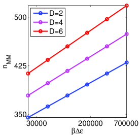
Figure 3: (color online) Linear-log plot of the number of matrix matrix multiplications $n_{\mathrm{MM}}$ versus $\beta\Delta\epsilon$. $n_{\mathrm{MM}}$ depends logarithmically on $\beta\Delta\epsilon$ with a small constant prefactor.

The potential $V$ is given by a sum of Gaussians centered at the atoms with width $\sigma=1.32\text{\AA}$ and depth $V_{0}=13.6\mathrm{eV}$. The kinetic energy is discretized using a simple 3-point finite difference formula, resulting in a Hamiltonian $\boldsymbol{\mathrm{H}}$ with a discrete eigenvalue spectrum with lower and upper eigenvalues equal to $\epsilon_{-}=6.76\mathrm{eV}$ and $\epsilon_{+}=1959\mathrm{eV}$, respectively. Various temperatures from $1024\mathrm{K}$ to $32\mathrm{K}$ were tried. Figure 3 reports the linear-log graph of $n_{\mathrm{MM}}$, the number of matrix by matrix multiplications needed to evaluate the density matrix using our FOE, versus $\beta\Delta\epsilon$, with $\beta\Delta\epsilon$ plotted in a logarithmic scale. The logarithmic dependence can be clearly seen. The prefactor of the logarithmic dependence is rather small: when $\beta\Delta\epsilon$ is doubled, a number of additional matrix multiplications equal to $17$ is required to achieve two-digit accuracy ($D=2$), a number equal to $19$ is needed for $D=4$, and a number equal to $21$ is needed for $D=6$, respectively. The observed $D$-dependence of the number of matrix multiplications agrees well with the prediction in (23).

In order to assess the validity of the criterion for the number of matrix multiplications given in Eq. (23), we report in Table 1 the calculated relative energy error and relative density error, respectively, at different temperatures, when the number of matrix multiplications is bounded as in formula (23) using different values for $D$. The relative energy error, $\Delta\epsilon_{\mathrm{rel}}$, measures the accuracy in the calculation of the total electronic energy corresponding to the supercell $E=\operatorname{Tr}(\boldsymbol{\mathrm{\rho}}\boldsymbol{\mathrm{H}})$. It is defined as

$$\Delta\epsilon_{\mathrm{rel}}=\frac{\lvert\hat{E}-E\rvert}{\lvert E\rvert}.$$ (27)

Similarly the relative $L^{1}$ error in the density function in real space is defined as

$$\Delta\rho_{\mathrm{rel}}=\frac{\operatorname{Tr}{\lvert\boldsymbol{\mathrm{\hat{\rho}}}-\boldsymbol{\mathrm{\rho}}\rvert}}{\operatorname{Tr}{\boldsymbol{\mathrm{\rho}}}}.$$ (28)

Because $\operatorname{Tr}{\boldsymbol{\mathrm{\rho}}}=N_{\mathrm{e}}$, where $N_{\mathrm{e}}$ is the total number of electrons in the supercell, $\Delta\rho_{\mathrm{rel}}$ is the same as the $L^{1}$ density error per electron. Table 1 shows that for all the values of $\beta\Delta\epsilon$, our algorithm gives a numerical accuracy that is even better than the target accuracy $D$. This is not surprising because our theoretical analysis was based on the most conservative error estimates.

IV.2 Periodic three dimensional tight-binding model

In this example we consider a periodic three dimensional single-band tight-binding Hamiltonian in a simple cubic lattice. The Hamiltonian, which can be viewed as the discretized form of a free-particle Hamiltonian, is given in second quantized notation by:

$$\boldsymbol{\mathrm{H}}=-t\sum_{<i,j>}c_{i}^{+}c_{j},$$ (29)

where the sum includes the nearest neighbors only. Choosing a value of $2.27\mathrm{eV}$ for the hopping parameter $t$ the band extrema occur at $\epsilon_{+}=13.606\mathrm{eV}$, and at $\epsilon_{-}=-13.606\mathrm{eV}$, respectively. In the numerical calculation we consider a periodically repeated supercell with $1000$ sites and chose a value of $100K$ for the temperature. Table 2 shows the dependence of $n_{\mathrm{MM}},\ \Delta\epsilon_{\mathrm{rel}},$ and $\Delta\rho_{\mathrm{rel}}$ on the chemical potential $\mu$, for different $D$ choices. Compared to the previous one dimensional example in which $\beta\Delta\epsilon$ was as large as $7.12\times 10^{5}$, here $\beta\Delta\epsilon=1600$ due to the much smaller spectral width of the tight-binding Hamiltonian. When $\mu=0$ the chemical potential lies exactly in the middle of the spectrum. This symmetry leads to a relative error as low as $10^{-19}$ for the density function.

IV.3 Three dimensional disordered Anderson model

In this example we consider an Anderson model with on-site disorder on a simple cubic lattice. The Hamiltonian is given by

$$\boldsymbol{\mathrm{H}}=-t\sum_{<i,j>}c_{i}^{+}c_{j}+\sum_{i}\epsilon_{i}c_{i}^{+}c_{i}.$$ (30)

This Hamiltonian contains random on-site energies $\epsilon_{i}$ uniformly distributed in the interval $[-1.13\mathrm{eV},1.13\mathrm{eV}]$, and we use the same hopping parameter $t$ as in the previous (ordered) example. In the numerical calculation we consider, as before, a supercell with $1000$ sites with periodic boundary conditions, and choose again a temperature of $100\mathrm{K}$. In one realization of disorder corresponding to a particular set of random on-site energies, the spectrum has extrema at $\epsilon_{+}=13.619\mathrm{eV}$ and at $\epsilon_{-}=-13.676\mathrm{eV}$. The effect of disorder on the density function is remarkable: while in the periodic tight-binding case the density was uniform, having the same constant value at all the lattice sites, now the density is a random function in the lattice sites within the supercell. Table 3 reports for the disordered model the same data that were reported in Table 2 for the ordered model. We see that the accuracy of our numerical FOE is the same in the two cases, irrespective of disorder. The only difference is that the super convergence due to symmetry for $\mu=0$ no longer exists in the disordered case.

V Conclusion

We proposed a multipole representation for the Fermi operator. Based on this expansion, a rather simple and efficient algorithm was developed for electronic structure analysis. We have shown that the number of number of matrix by matrix multiplication that are needed scales as $(\ln\beta\Delta\epsilon)\cdot(\ln\ln\beta\Delta\epsilon)$ with very small overhead. Numerical examples show that the algorithm is promising and has the potential to be applied to metallic systems.

We have only considered the number of matrix matrix multiplications as a measure for the computational cost. The real operational count should of course take into account the cost of multiplying two matrices, and hence depends on how the matrices are represented. This is work in progress.

Appendix A Mittag-Leffler’s theorem and pole expansion for hyperbolic tangent function

To obtain the pole expansion for hyperbolic tangent function $\tanh(z)$, we need a special case of the general Mittag-Leffler’s theorem on the expansions of meromorphic functions (see, for example, Jeffreys and Jeffreys (1956); Ahlfors (1978)).

Theorem 1 (Mittag-Leffler).

If a function $f(z)$ analytic at the origin has no singularities other than poles for finite $z$, and if we can choose a sequence of contours $C_{m}$ about $z=0$ tending to infinity, such that $\lvert f(z)\rvert\leq M$ on $C_{m}$ and $\int_{C_{m}}\lvert\,\mathrm{d}z/z\rvert$ is uniformly bounded, then we have

$$f(z)=f(0)+\lim_{m\to\infty}\{P_{m}(z)-P_{m}(0)\},$$ (31)

where $P_{m}(z)$ is the sum of the principal parts of $f(z)$ at all poles within $C_{m}$.

For $\tanh(z)=\dfrac{\exp(z)-\exp(-z)}{\exp(z)+\exp(-z)}$, it is analytic at the origin and $\tanh(0)=0$. The function has simple poles at $z_{l}=(l-1/2)\pi i,\ l\in\mathbb{Z}$ with principle parts $(z-z_{l})^{-1}$. Let us take the contours as

$$C_{m}=\{x\pm im\pi\mid\lvert x\rvert\leq m\pi\}\cup\{\pm m\pi+iy\mid\lvert y\rvert\leq m\pi\},\quad m\in\mathbb{Z}_{+},$$

it is then easy to verify that $C_{m}$ satisfy the conditions in Theorem 1. According to Theorem 1,

$$\tanh(z)=\tanh(0)+\lim_{m\to\infty}\sum_{l=-m+1}^{m}\Bigl{(}\frac{1}{z-z_{l}}+\frac{1}{z_{l}}\Bigr{)}.$$ (32)

By symmetry of $z_{l}$, the second term within the brackets cancels, and we arrive at (3).

Acknowledgement: We thank M. Ceriotti and M. Parrinello for useful discussions. This work was partially supported by DOE under Contract No. DE-FG02-03ER25587 and by ONR under Contract No. N00014-01-1-0674 (W. E, L. L., and J. L.), and by DOE under Contract No. DE-FG02-05ER46201 and NSF-MRSEC Grant DMR-02B706 (R. C. and L. L.).

T	$\beta\Delta\epsilon$	$\Delta\epsilon_{\mathrm{rel}}$			$\Delta\rho_{\mathrm{rel}}$
		$D=2$	$D=4$	$D=6$	$D=2$	$D=4$	$D=6$
$1024K$	$2.22\times 10^{4}$	$1.64\times 10^{-3}$	$5.98\times 10^{-6}$	$3.31\times 10^{-8}$	$4.21\times 10^{-4}$	$2.23\times 10^{-6}$	$1.50\times 10^{-8}$
$512K$	$4.44\times 10^{4}$	$1.73\times 10^{-3}$	$6.49\times 10^{-6}$	$3.70\times 10^{-8}$	$4.63\times 10^{-4}$	$2.52\times 10^{-6}$	$1.74\times 10^{-8}$
$256K$	$8.89\times 10^{4}$	$1.78\times 10^{-3}$	$6.83\times 10^{-6}$	$3.96\times 10^{-8}$	$4.77\times 10^{-4}$	$2.62\times 10^{-6}$	$1.81\times 10^{-8}$
$128K$	$1.78\times 10^{5}$	$1.74\times 10^{-3}$	$6.55\times 10^{-6}$	$3.75\times 10^{-8}$	$5.04\times 10^{-4}$	$2.80\times 10^{-6}$	$1.95\times 10^{-8}$
$64K$	$3.56\times 10^{5}$	$1.75\times 10^{-3}$	$6.62\times 10^{-6}$	$3.80\times 10^{-8}$	$4.92\times 10^{-4}$	$2.70\times 10^{-6}$	$1.86\times 10^{-8}$
$32K$	$7.12\times 10^{5}$	$1.76\times 10^{-3}$	$6.66\times 10^{-6}$	$3.82\times 10^{-8}$	$4.84\times 10^{-4}$	$2.64\times 10^{-6}$	$1.80\times 10^{-8}$

Table 1: One dimensional Hamiltonian model of Section IV.1. Relative energy error $\Delta\epsilon_{\mathrm{rel}}$ and relative $L^{1}$ density error $\Delta\rho_{\mathrm{rel}}$ for a large range of values of $\beta\Delta\epsilon$ and several values of $D$.

$\mu$	$D=4$			$D=8$
	$n_{\mathrm{MM}}$	$\Delta\epsilon_{\mathrm{rel}}$	$\Delta\rho_{\mathrm{rel}}$	$n_{\mathrm{MM}}$	$\Delta\epsilon_{\mathrm{rel}}$	$\Delta\rho_{\mathrm{rel}}$
$-10.88\mathrm{eV}$	$320$	$4.09\times 10^{-9}$	$2.31\times 10^{-10}$	$376$	$2.27\times 10^{-13}$	$2.37\times 10^{-14}$
$-5.44\mathrm{eV}$	$308$	$1.48\times 10^{-9}$	$3.15\times 10^{-11}$	$356$	$4.77\times 10^{-13}$	$2.52\times 10^{-15}$
$0.00\mathrm{eV}$	$305$	$1.55\times 10^{-9}$	$6.26\times 10^{-19}$	$357$	$2.98\times 10^{-15}$	$6.26\times 10^{-19}$
$5.44\mathrm{eV}$	$308$	$1.45\times 10^{-8}$	$1.34\times 10^{-12}$	$356$	$5.36\times 10^{-13}$	$1.07\times 10^{-16}$
$10.88\mathrm{eV}$	$320$	$1.69\times 10^{-8}$	$1.78\times 10^{-13}$	$376$	$1.09\times 10^{-12}$	$1.80\times 10^{-17}$

Table 2: Three dimensional periodic tight binding model of Section IV.2. Number of matrix matrix multiplications $n_{\mathrm{MM}}$, relative energy error $\Delta\epsilon_{\mathrm{rel}}$, and relative $L^{1}$ density error $\Delta\rho_{\mathrm{rel}}$. For $\mu=0$, the algorithm achieves machine accuracy for the absolute error of the density function as a consequence of symmetry.

$\mu$	$D=4$			$D=8$
	$n_{\mathrm{MM}}$	$\Delta\epsilon_{\mathrm{rel}}$	$\Delta\rho_{\mathrm{rel}}$	$n_{\mathrm{MM}}$	$\Delta\epsilon_{\mathrm{rel}}$	$\Delta\rho_{\mathrm{rel}}$
$-10.88\mathrm{eV}$	$320$	$5.16\times 10^{-9}$	$1.72\times 10^{-10}$	$376$	$3.16\times 10^{-13}$	$2.59\times 10^{-14}$
$-5.44\mathrm{eV}$	$308$	$4.75\times 10^{-9}$	$2.43\times 10^{-11}$	$356$	$3.71\times 10^{-13}$	$1.48\times 10^{-15}$
$0.00\mathrm{eV}$	$305$	$8.08\times 10^{-10}$	$9.50\times 10^{-13}$	$357$	$1.76\times 10^{-14}$	$2.39\times 10^{-17}$
$5.44\mathrm{eV}$	$308$	$1.01\times 10^{-8}$	$1.22\times 10^{-12}$	$356$	$3.57\times 10^{-13}$	$8.05\times 10^{-17}$
$10.88\mathrm{eV}$	$320$	$1.30\times 10^{-8}$	$1.56\times 10^{-13}$	$376$	$9.56\times 10^{-13}$	$1.83\times 10^{-17}$

Table 3: Three dimensional Anderson model with on-site disorder discussed in Section IV.3. Number of matrix matrix multiplications $n_{\mathrm{MM}}$, relative energy error $\Delta\epsilon_{\mathrm{rel}}$, and relative $L^{1}$ density error $\Delta\rho_{\mathrm{rel}}$.

References

- Baroni and Giannozzi (1992) S. Baroni and P. Giannozzi, Europhys. Lett. 17, 547 (1992).
- Goedecker and Colombo (1994) S. Goedecker and L. Colombo, Phys. Rev. Lett. 73, 122 (1994).
- Goedecker and Teter (1995) S. Goedecker and M. Teter, Phys. Rev. B 51, 9455 (1995).
- Goedecker (1999) S. Goedecker, Rev. Mod. Phys. 71, 1085 (1999).
- Krajewski and Parrinello (2005) F. Krajewski and M. Parrinello, Phys. Rev. B 71, 233105 (2005).
- Krajewski and Parrinello (2006a) F. Krajewski and M. Parrinello, Phys. Rev. B 73, 41105 (2006a).
- Krajewski and Parrinello (2006b) F. Krajewski and M. Parrinello, Phys. Rev. B 74, 125107 (2006b).
- Krajewski and Parrinello (2007) F. Krajewski and M. Parrinello, Phys. Rev. B 75, 235108 (2007).
- Ceriotti et al. (2008a) M. Ceriotti, T. Kühne, and M. Parrinello, J. Chem. Phys 129, 024707 (2008a).
- Ceriotti et al. (2008b) M. Ceriotti, T. Kühne, and M. Parrinello, arXiv:0809.2232v1 (2008b).
- Liang et al. (2003) W. Liang, C. Saravanan, Y. Shao, R. Baer, A. T. Bell, and M. Head-Gordon, J. Chem. Phys. 119, 4117 (2003).
- Liang et al. (2004) W. Liang, R. Baer, C. Saravanan, Y. Shao, A. T. Bell, and M. Head-Gordon, J. Comput. Phys. 194, 575 (2004).
- Mahan (2000) G. Mahan, Many-particle Physics (Plenum Pub Corp, 2000).
- Greengard and Rokhlin (1987) L. Greengard and V. Rokhlin, J. Comput. Phys. 73, 325 (1987).
- Jeffreys and Jeffreys (1956) H. Jeffreys and B. S. Jeffreys, Methods of mathematical physics (Cambridge, at the University Press, 1956), 3rd ed.
- Ahlfors (1978) L. V. Ahlfors, Complex analysis (McGraw-Hill Book Co., New York, 1978), 3rd ed.
- Baer and Head-Gordon (1997) R. Baer and M. Head-Gordon, J. Chem. Phys. 107, 10003 (1997).