$K_{l3}$ and pion form factors using partially twisted boundary conditions

Abstract:

We compute the $K_{\ell 3}$ and pion form factors using partially twisted boundary conditions. The twists are chosen so that the $K_{\ell 3}$ form factors are calculated directly at zero momentum transfer $(q^{2}=0)$, removing the need for a $q^{2}$ interpolation, while the pion form factor is determined at values of $q^{2}$ close to $q^{2}=0$. The simulations are performed on an ensemble of the RBC/UKQCD collaboration’s gauge configurations with Domain Wall Fermions and the Iwaski gauge action with an inverse lattice spacing of 1.73(3) GeV. Simulating at a single pion mass of 330 MeV, we find the pion charge radius to be $\langle r^{2}\rangle_{\rm 330\,MeV}=0.354(31)\,{\rm fm}^{2}$ which, using NLO SU(2) chiral perturbation theory, translates to a value of $\langle r_{\pi}^{2}\rangle=0.418(31)\,{\rm fm}^{2}$ for a physical pion. For the value of the $K_{\ell 3}$ form factor, $f_{K\pi}^{+}(q^{2})$, determined directly at $q^{2}=0$, we find a value of $f_{K\pi}^{+}(0)=0.9742(41)$ at this particular quark mass, which agrees well with our earlier result (0.9774(35)) obtained using the standard, indirect method.

Edinburgh 2008/48
SHEP-0835

1 Introduction

Over the last two years as part of our Domain Wall Fermion (DWF) physics programme we have been looking at the $K\rightarrow\pi\ell\nu_{\ell}$ ($K_{\ell 3}$) form factor at zero momentum transfer. Since the experimental rate for $K_{\ell 3}$ decays is proportional to $|V_{us}|^{2}|f_{K\pi}^{+}(0)|^{2}$, a lattice calculation of the form factor, $f_{K\pi}^{+}(q^{2})$ at $q^{2}=0$, provides an excellent avenue for the determination of the Cabibbo-Kobayashi-Maskawa (CKM) [1] quark mixing matrix element, $|V_{us}|$.

The uncertainty in the unitarity relation of the CKM matrix $\left|V_{ud}\right|^{2}+\left|V_{us}\right|^{2}=1$ (we ignore $\left|V_{ub}\right|$ since this is very small), is dominated by the precision of $\left|V_{us}\right|$. In Fig. 1 we show the latest determinations of $|V_{ud}|$ [2] and $\left|V_{us}\right|$ [3]. For comparison, we also show the unitarity relation. Since it is important to establish unitarity with the best precision possible, it is essential that we decrease the error in $|V_{us}|$.

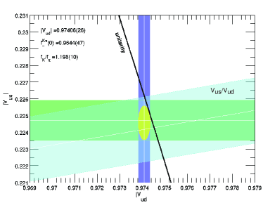
Figure 1: Bands showing the current limits on $|V_{ud}|$ [2], and $|V_{us}|$[3].

The value of $f_{K\pi}^{+}(0)$ used in determining $\left|V_{us}\right|$ in figure 1 was determined using standard methods [4, 5] involving periodic boundary conditions in the recent paper [3]. There, the $K_{\ell 3}$ form factor is calculated at $q^{2}_{max}=(m_{K}-m_{\pi})^{2}$ and several negative values of $q^{2}$ for a variety of quark masses. This allows for an interpolation of the results to $q^{2}=0$. The form factor is then chirally extrapolated to the physical pion and kaon masses. The final result for $f_{K\pi}^{+}(0)$ quoted is then [3] $f_{K\pi}^{+}(0)=0.9644(33)(34)(14)$ where the first error is statistical, and the second and third are estimates of the systematic errors due to the choice of parametrisation for the interpolation and lattice artefacts, respectively. This gives us a value of $\left|V_{us}\right|=0.2249(14)$.

More recently, we have developed a method that uses partially twisted boundary conditions to calculate the $K_{\ell 3}$ form factor directly at $q^{2}=0$ [6], thereby removing the systematic error due to the choice of parametrisation for the interpolation in $q^{2}$. We have also used partially twisted bc’s to calculate the pion form factor at values of $q^{2}$ below the minimum value obtainable with periodic bc’s. In contrast to recent studies this allows for a direct evaluation of the charge radius of the pion. The method was developed and tested in [6] and now applied in a simulation with parameters much closer to the physical point.

In this paper we discuss our findings for the pion form factor from [7] and our progress in improving the precision of our result for $f_{K\pi}^{+}(0)$ from [3] using partially twisted boundary conditions.

2 Simulation Parameters

The computations are performed using an ensemble with light quark mass $am_{u}=am_{d}=0.005$ and strange quark mass $am_{s}=0.04$ from a set of $N_{f}=2+1$ flavour DWF configurations with $(L/a)^{3}\times T/a\times L_{s}=24^{3}\times 64\times 16$ which were jointly generated by the UKQCD/RBC collaborations [8] using the QCDOC computer. The gauge configurations were generated with the Iwasaki gauge action with an inverse lattice spacing of $a^{-1}=1.729(28)\mathrm{GeV}$. The resulting pion and kaon masses are $m_{\pi}\approx 330\mathrm{MeV}$ and $m_{K}\approx 575\mathrm{MeV}$, respectively.

In this work we use single time-slice stochastic sources [10], for which the elements of the source are randomly drawn from a distribution $\mathcal{D}=\mathbb{Z}(2)\otimes\mathbb{Z}(2)$ which contains random $\mathbb{Z}(2)$ numbers in both its real and imaginary parts. With sources of this form we find that the computational cost of calculating quark propagators is reduced by a factor of 12. For more details on the simulations, see [7].

3 The Form Factors

Here we briefly outline the main features of our method and we refer the reader to our earlier papers for more details [3, 6, 7].

The matrix element of the vector current between initial and final state pseudoscalar mesons $P_{i}$ and $P_{f}$, is in general decomposed into two invariant form factors:

$$\langle{P_{f}(p_{f})}|V_{\mu}|{P_{i}(p_{i})}\rangle=f^{+}_{P_{i}P_{f}}(q^{2})(p_{i}+p_{f})_{\mu}+f^{-}_{P_{i}P_{f}}(q^{2})(p_{i}-p_{f})_{\mu},$$ (1)

where $q^{2}=-Q^{2}=(p_{i}-p_{f})^{2}$. For $K\rightarrow\pi$, $V_{\mu}=\bar{s}\gamma_{\mu}u$, $P_{i}=K$ and $P_{f}=\pi$. For $\pi\rightarrow\pi$, $V_{\mu}=\frac{2}{3}\bar{u}\gamma_{\mu}u-\frac{1}{3}\bar{d}\gamma_{\mu}d$, $P_{i}=P_{f}=\pi$ and from vector current conservation, $f^{-}_{\pi\pi}(q^{2})=0$. The form factors $f^{+}_{P_{i}P_{f}}(q^{2})$ and $f^{-}_{P_{i}P_{f}}(q^{2})$ contain the non-perturbative QCD effects and hence are ideally suited for a determination in lattice QCD.

In a finite volume with spatial extent $L$ and periodic boundary conditions for the quark fields, momenta are discretised in units of $2\pi/L$. As a result, the minimum non-zero value of $Q^{2}$ for the pion form factor in our simulation is $q^{2}_{\rm min}\approx-0.15\ {\rm GeV}^{2}$, while for the $K\to\pi$ form factor

$$q^{2}=(E_{K}(\vec{p}_{i})-E_{\pi}(\vec{p}_{f}))^{2}-(\vec{p}_{i}-\vec{p}_{f})^{2}\ .$$ (2)

For $\vec{p}_{i}=0$ and $2\pi/L$ with $\vec{p}_{f}=0$, we have $q^{2}\approx 0.06\ {\rm GeV}^{2}$ and $-0.05\ {\rm GeV}^{2}$, respectively, presenting the need for an interpolation in order to extract the result of the form factor, $f_{K\pi}^{+}$, at $q^{2}=0$.

In order to reach small momentum transfers for the pion form factor and $q^{2}=0$ for the $K\to\pi$ form factors, we use partially twisted boundary conditions [11, 12], combining gauge field configurations generated with sea quarks obeying periodic boundary conditions with valence quarks with twisted boundary conditions [11, 12, 13, 14, 15, 16, 17]. The valence quarks, $q$, satisfy

$$q(x_{k}+L)=e^{i\theta_{k}}q(x_{k}),\qquad(k=1,2,3)\,,$$ (3)

where $\vec{\theta}$ is the twisting angle.

Our method is decribed in detail in [6, 7] and proceeds by setting $\vec{\theta}=0$ for the spectator quark, denoted by $q_{3}$ in the above diagram. We are then able to vary the twisting angles, $\vec{\theta}_{i}$ and $\vec{\theta_{f}}$, of the quarks before $(q_{2})$ and after $(q_{1})$ the insertion of the current, respectively. The momentum transfer between the initial and final state mesons is now

$$q^{2}=(E_{i}(\vec{p}_{i},\vec{\theta}_{i})-E_{f}(\vec{p}_{f},\vec{\theta}_{f}))^{2}-((\vec{p}_{i}+\vec{\theta}_{i}/L)-(\vec{p}_{f}+\vec{\theta}_{f}/L))^{2}\ ,$$ (4)

where $E(\vec{p},\vec{\theta})=\sqrt{m^{2}+(\vec{p}+\vec{\theta}/L)^{2}}$. Hence it is possible to choose $\vec{\theta}_{i}$ and $\vec{\theta}_{f}$ such that $q^{2}=0$, which from now on we refer to as $\vec{\theta}_{K}$ and $\vec{\theta}_{\pi}$ for when we twist a quark in the Kaon and Pion, respectively.

In order to extract the matrix elements (1) from a lattice simulation, we consider ratios of three- and two-point correlation functions. For the pion form factor, we consider the ratios given in Eqs. (3.4) and (3.5) in [7], while for the $K\to\pi$ form factors, we consider the following ratios

$$\begin{array}[]{rcl}R_{1,\,P_{i}P_{f}}(\vec{p}_{i},\vec{p}_{f})&{=}&4\sqrt{E_{i}E_{f}}\,\sqrt{\frac{C_{P_{i}P_{f}}(t,\vec{p}_{i},\vec{p}_{f})\,C_{P_{f}P_{i}}(t,\vec{p}_{f},\vec{p}_{i})}{C_{P_{i}}(t_{\rm sink},\vec{p}_{i})\,C_{P_{f}}(t_{\rm sink},\vec{p}_{f})}},\\[11.38109pt] R_{3,\,P_{i}P_{f}}(\vec{p}_{i},\vec{p}_{f})&=&4{\sqrt{E_{i}E_{f}}}\,\frac{C_{P_{i}P_{f}}(t,\vec{p}_{i},\vec{p}_{f})}{C_{P_{f}}(t_{\rm sink},\vec{p}_{f})}\,\sqrt{\frac{C_{P_{i}}(t_{\rm sink}-t,\vec{p}_{i})\,C_{P_{f}}(t,\vec{p}_{f})\,C_{P_{f}}(t_{\rm sink},\vec{p}_{f})}{C_{P_{f}}(t_{\rm sink}-t,\vec{p}_{f})\,C_{P_{i}}(t,\vec{p}_{i})\,C_{P_{i}}(t_{\rm sink},\vec{p}_{i})}}\,.\end{array}$$ (5)

We deviate slightly from the method outlined in [6] for extracting $f_{K\pi}^{0}(0)$ from the ratios. Previously we considered only the time-component of the vector current and solved for $f_{K\pi}^{0}(0)=f_{K\pi}^{+}(0)$ via the linear combination

$$f_{K\pi}^{0}(0)=\frac{R_{\alpha,K\pi}(\vec{p}_{K},\vec{0})(m_{K}-E_{\pi})-R_{\alpha,K\pi}(\vec{0},\vec{p}_{\pi})(E_{K}-m_{\pi})}{(E_{K}+m_{\pi})(m_{K}-E_{\pi})-(m_{K}+E_{\pi})(E_{K}-m_{\pi})}\qquad(\alpha=1,2,3)\,.$$ (6)

This, however, is just one of many expressions that can be obtained when we solve the system of simultaneous equations that are obtained when we consider all components of the vector current, $V_{\mu}$, rather than just $V_{4}$ that was considered in [6]

$$R_{\alpha,K\pi}(\vec{\theta}_{K},\vec{0},V_{4}) = f_{K\pi}^{+}(0)\,(E_{K}+m_{\pi})+f_{K\pi}^{-}(0)\,(E_{K}-m_{\pi})$$

$$R_{\alpha,K\pi}(\vec{0},\vec{\theta}_{\pi},V_{4}) = f_{K\pi}^{+}(0)\,(m_{K}+E_{\pi})+f_{K\pi}^{-}(0)\,(m_{K}-E_{\pi})$$

$$R_{\alpha,K\pi}(\vec{\theta}_{K},\vec{0},V_{i}) = f_{K\pi}^{+}(0)\,\theta_{K,i}+f_{K\pi}^{-}(0)\,\theta_{K,i}$$

$$R_{\alpha,K\pi}(\vec{0},\vec{\theta}_{\pi},V_{i}) = f_{K\pi}^{+}(0)\,\theta_{\pi,i}-f_{K\pi}^{-}(0)\,\theta_{\pi,i}\ .$$ (7)

We can now proceed to solve this overdetermined system of equations via $\chi^{2}$ minimisation.

4 Pion form factor results

In Fig. 2 we show our results for the form factor $f^{\pi\pi}(q^{2})$ for a pion with $m_{\pi}=330\,\mathrm{MeV}$ for a range of values of $q^{2}$ both using periodic bc’s and partially twisted bc’s (set A and sets B&C respectively in the left plot of figure). The vertical dashed line indicates the smallest momentum transfer available on this lattice with periodic bc’s. The (blue) dashed line is the result of a pole-dominance fit to our data points, while the (red) dot-dashed curve is obtained from the result of QCDSF [18] evaluated at $m_{\pi}=330$ MeV.

\psfrag{xlabel}[c][b][1][0]{\small$Q^{2}[\,\mathrm{GeV}^{2}]$}\psfrag{ylabel}[c][t][1][0]{\small$f^{\pi\pi}(q^{2})$}\includegraphics[width=151.76964pt,angle={-90}]{fpipi_pole.eps}

\psfrag{xlabel}[c][bc][1][0]{\small$Q^{2}[\,\mathrm{GeV}^{2}]$}\psfrag{ylabel}[c][t][1][0]{\small$f^{\pi\pi}(q^{2})$}\psfrag{exp}[l][lc][1][0]{\tiny experimental data NA7}\psfrag{330MeV}[l][lc][1][0]{\tiny lattice data for $m_{\pi}=330\,\mathrm{MeV}$}\psfrag{NLO330MeV}[l][ll][1][0]{\tiny$\mathrm{SU}(2)$ NLO lattice-fit; $m_{\pi}=330\,\mathrm{MeV}$}\psfrag{NLO139.57MeV}[l][ll][1][0]{\tiny$\mathrm{SU}(2)$ NLO lattice-fit; $m_{\pi}=139.57\,\mathrm{MeV}$}\psfrag{444OOOOOOOOOOOOOOOOOOOO}[l][lc][1][0]{\tiny$1+\frac{1}{6}\langle r^{2}_{\pi}\rangle^{\rm PDG}Q^{2}$}\includegraphics[width=151.76964pt,angle={-90}]{final.eps}

Figure 2: $f^{\pi\pi}(q^{2})$ from a $24^{3}\times 64$ lattice with $m_{\pi}=330$ MeV using partially twisted bc’s.

On the right of Fig. 2 we have a zoom into the low $Q^{2}=-q^{2}$ region. The triangles are our lattice data points for a pion with $m_{\pi}=330\,\mathrm{MeV}$, and the magenta diamonds are experimental data points for the physical pion.

Because our values of $Q^{2}$ are very small, we apply NLO chiral perturbation theory (ChPT). In NLO ChPT, the pion form factor depends only on a single low energy constant (LEC) ($L_{9}^{r}$ for SU(3), or $l_{6}^{r}$ for SU(2))

$$f^{\pi\pi}_{\mathrm{SU}(2),\mathrm{NLO}}(q^{2}) = 1+\frac{1}{f^{2}}\left[-2l_{6}^{r}\,q^{2}+4\tilde{\mathcal{H}}(m_{\pi}^{2},q^{2},\mu^{2})\right]$$ (8)

$$f^{\pi\pi}_{\mathrm{SU}(3),\mathrm{NLO}}(q^{2}) = 1+\frac{1}{f_{0}^{2}}\left[4L_{9}^{r}\,q^{2}+4\tilde{\mathcal{H}}(m_{\pi}^{2},q^{2},\mu^{2})+2\tilde{\mathcal{H}}(m_{K}^{2},q^{2},\mu^{2})\right]$$ (9)

where

$$\tilde{\mathcal{H}}(m^{2},q^{2},\mu^{2})=\frac{m^{2}H(q^{2}/m^{2})}{32\pi^{2}}-\frac{q^{2}}{192\pi^{2}}\log\frac{m^{2}}{\mu^{2}}$$ (10)

and

$$H(x)\equiv-\frac{4}{3}+\frac{5}{18}x-\frac{(x-4)}{6}\sqrt{\frac{x-4}{x}}\log\left(\frac{\sqrt{(x-4)/x}\,+1}{\sqrt{(x-4)/x}\,-1}\right)$$ (11)

with $H(x)=-x/6+O(x^{3/2})$ for small $x$. Provided our pion mass is light enough, we can use the $q^{2}$ dependence of $f^{\pi\pi}(q^{2})$ to extract this LEC. The grey dashed curve on the right hand of Fig. 2 shows our SU(2) fit to the $m_{\pi}=330\,\mathrm{MeV}$ pion form factor data.

Once the LEC is determined from this fit, we insert the physical pion mass in (8) to obtain the solid blue curve. In addition we also represent the PDG world average [2] for the charge radius using the black dashed line. Our best estimate for the pion charge radius comes from the SU(2) NLO ChPT fit to the three lowest $Q^{2}$ points and is

$$\langle r_{\pi}^{2}\rangle=0.418(31)\,\rm{fm^{2}}\ .$$ (12)

The fact that our result is in agreement with experiment, $\langle r_{\pi}^{2}\rangle=0.452(11)\,\rm{fm^{2}}$ [2], gives us confidence that we are in a regime where chiral perturbation theory is applicable.

5 $K_{l3}$ form factor results

As explained in Sec. 3, we calculate the $K\rightarrow\pi$ form factor directly at $q^{2}=0$ by setting the Kaon and Pion in turn to be at rest, while twisting the other one such that $q^{2}=0$. We refer to these twist angles as $\theta_{\pi}$ and $\theta_{K}$, respectively. We then get the following equations:

$$\langle K(p_{K})|V_{\mu}|\pi(0)\rangle = f_{K\pi}^{+}(0)p_{K,\mu}-f_{K\pi}^{-}(0)p_{K,_{\mu}}$$

$$\langle K(0)|V_{\mu}|\pi(p_{\pi})\rangle = f_{K\pi}^{+}(0)p_{\pi,\mu}+f_{K\pi}^{-}(0)p_{\pi,_{\mu}}$$ (13)

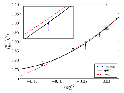
Figure 3: $K_{\ell 3}$ form factor, $f_{K\pi}^{0}(q^{2})$, evaluated at $q^{2}=0$ directly using twisted boundary conditions. Results are compared with data at $q^{2}\neq 0$ and fits from [3]

By simply solving the simultaneous equations for each of the $\mu$ components separately we find that the errors in $f_{K\pi}^{+}(0)$ and $f_{K\pi}^{-}(0)$, are much larger than the errors in the matrix elements. We have managed to circumvent this by looking at all the $\mu$ components simultaneously, and then performing a $\chi^{2}$ minimisation on the overdetermined system of equations to find the values of $f_{K\pi}^{+}(0)$ and $f_{K\pi}^{-}(0)$ that best fit the equations.

To obtain the matrix elements (13), we consider different combinations of $R_{1}$ and $R_{3}$ (5). We find that all combinations lead to consistent results, with the best combination being that we use $R_{3}$ for all matrix elements except for the case where the pion is twisted and we are considering the $4^{\rm th}$ component of the vector current. Using this set up, we obtain our preliminary results for $f^{+}_{K\pi}(0)$ and $f^{-}_{K\pi}(0)$ (for a pion mass of $m_{\pi}=330\,\mathrm{MeV}$)

$$f^{+}_{K\pi}(0)=0.9742(41)\,,\quad f^{-}_{K\pi}(0)=-0.113(12)\ .$$ (14)

Our result for $f^{+}_{K\pi}(0)=f^{0}_{K\pi}(0)$ is shown in Fig. 3 where we compare with the previous determinations in [3] which used pole $f^{+}_{pole}(0)=0.9774(35)$ and quadratic $f^{+}_{quad}(0)=0.9749(59)$ functions to interpolate between $q^{2}_{max}$ and negative values of $q^{2}$. In our previous result, $f_{K\pi}^{+}(0)=0.9644(33)(34)(14)$, these were combined, taking a systematic error of (34) for the model dependence. This contribution to the error has been eliminated in our new calculation.

We conclude that using partially twisted bc’s for the $K_{\ell 3}$ form factor, is an improvement on the conventional method as it removes a source of systematic error, while keeping comparable statistical errors. Another source of systematic error in our result in [3] is due to the slight difference between our simulated strange quark mass ($am_{s}+am_{\rm res}\simeq 0.043$) and the physical strange quark ($am_{s}+am_{\rm res}\simeq 0.037$) [8], and we are in the process of determining the effect this has on our result through a simulation with a partially quenched strange quark mass of $am_{s}+am_{\rm res}\simeq 0.033$. We also plan to combine our results with the latest expressions from chiral perturbation theory [19].

References

- [1] N. Cabibbo, Phys. Rev. Lett. 10 (1963) 531; M. Kobayashi and T. Maskawa, Prog. Theor. Phys. 49 (1973) 652.
- [2] W. M. Yao et al. [Particle Data Group], J. Phys. G 33 (2006) 1.
- [3] P. A. Boyle et al. [RBC/UKQCD], Phys. Rev. Lett. 100 (2008) 141601 [arXiv:0710.5136 [hep-lat]].
- [4] D. Becirevic et al., Nucl. Phys. B 705 (2005) 339 [arXiv:hep-ph/0403217].
- [5] C. Dawson, T. Izubuchi, T. Kaneko, S. Sasaki and A. Soni, Phys. Rev. D 74 (2006) 114502 [arXiv:hep-ph/0607162].
- [6] P. A. Boyle et al. [RBC/UKQCD], JHEP 0705 (2007) 016 [arXiv:hep-lat/0703005].
- [7] P. A. Boyle et al. [RBC/UKQCD], JHEP 0807 (2008) 112 [arXiv:0804.3971 [hep-lat]].
- [8] C. Allton et al. [RBC/UKQCD], arXiv:0804.0473 [hep-lat].
- [9] S. Simula [ETMC], PoS LAT2007 (2007) 371 [arXiv:0710.0097 [hep-lat]].
- [10] P. A. Boyle, A. Juttner, C. Kelly and R. D. Kenway, JHEP 0808 (2008) 086 [arXiv:0804.1501 [hep-lat]].
- [11] C. T. Sachrajda and G. Villadoro, Phys. Lett. B 609 (2005) 73 [arXiv:hep-lat/0411033].
- [12] P. F. Bedaque and J. W. Chen, Phys. Lett. B 616 (2005) 208 [arXiv:hep-lat/0412023].
- [13] P. F. Bedaque, Phys. Lett. B 593 (2004) 82 [arXiv:nucl-th/0402051].
- [14] G. M. de Divitiis, R. Petronzio and N. Tantalo, Phys. Lett. B 595 (2004) 408 [arXiv:hep-lat/0405002].
- [15] B. C. Tiburzi, Phys. Lett. B 617 (2005) 40 [arXiv:hep-lat/0504002].
- [16] J. M. Flynn, A. Juttner and C. T. Sachrajda [UKQCD], Phys. Lett. B 632 (2006) 313 [arXiv:hep-lat/0506016].
- [17] D. Guadagnoli, F. Mescia and S. Simula, Phys. Rev. D 73 (2006) 114504 [arXiv:hep-lat/0512020].
- [18] D. Brömmel et al. [QCDSF/UKQCD], Eur. Phys. J. C 51 (2007) 335 [arXiv:hep-lat/0608021].
- [19] J. M. Flynn and C. T. Sachrajda, arXiv:0809.1229 [hep-ph].